Linear optics and quantum maps

Linear optics and quantum maps

A. Aiello, G. Puentes, and J. P. Woerdman

Huygens Laboratory, Leiden University, P.O. Box 9504, 2300 RA Leiden, The Netherlands 共Received 17 November 2006; published 21 September 2007兲

We present a theoretical analysis of the connection between classical polarization optics and quantum mechanics of two-level systems. First, we review the matrix formalism of classical polarization optics from a quantum information perspective. In this manner the passage from the Stokes-Jones-Mueller description of classical optical processes to the representation of one- and two-qubit quantum operations, becomes straight-forward. Second, as a practical application of our classical-vs-quantum formalism, we show how two-qubit maximally entangled mixed states can be generated by using polarization and spatial modes of photons generated via spontaneous parametric down conversion.

DOI:10.1103/PhysRevA.76.032323 PACS number共s兲: 03.67.Mn, 03.65.Ud, 42.25.Ja

I. INTRODUCTION

Quantum computation and quantum information have been among the most popular branches of physics in the last decade 关1兴. One of the reasons for this interest is that the smallest unit of quantum information, the qubit, could be reliably encoded in photons that are easy to manipulate and virtually free from decoherence at optical frequencies关2,3兴. Thus, recently, there has been a growing interest in quantum information processing with linear optics关4–7兴 and several techniques to generate and manipulate optical qubits have been developed for different purposes ranging from, e.g., teleportation关8,9兴, to quantum cryptography关3兴, to quantum measurements of qubits states关10兴and processes关11兴, etc. In particular, Kwiat and co-workers关12,13兴were able to create and characterize arbitrary one- and two-qubit states, using polarization and frequency modes of photons generated via spontaneous parametric down conversion共SPDC兲 关14兴.

Manipulation of optical qubits is performed by means of linear optical instruments such as half- and quarter-wave plates, beam splitters, polarizers, mirrors, etc., and networks of these elements. Each of these devices can be thought as an object where incoming modes of the electromagnetic fields are turned into outgoing modes by a linear transformation. From a quantum information perspective, this transforms the state of qubits encoded in some degrees of freedom of the incoming photons, according to a completely positive mapE describing the action of the device. Thus, an optical instru-ment may be put in correspondence with a quantum map and vice versa. Such correspondence has been largely exploited

关7,12,13,15兴 and stressed关16,17兴by several authors. More-over, classical physics of linear optical devices is a textbook matter 关18,19兴, and quantum physics of elementary optical instruments has been studied extensively关20兴, as well. How-ever, surprisingly enough, a systematic exposition of the con-nection between classical linear optics and quantum maps is still lacking.

In this paper we aim to fill this gap by presenting a de-tailed theory of linear optical instruments from a quantum information point of view. Specifically, we establish a rigor-ous basis for the connection between quantum maps describ-ing one- and two-qubit physical processes operated by polarization-affecting optical instruments and the classical

matrix formalism of polarization optics. Moreover, we will use this connection to interpret some recent experiments in our group关21兴.

We begin in Sec. II by reviewing the classical theory of polarization-affecting linear optical devices. Then, in Sec. III we show how to pass, in a natural manner, from classical polarization-affecting optical operations to one-qubit tum processes. Such passage is extended to two-qubit quan-tum maps in Sec. IV. In Sec. V we furnish two explicit ap-plications of our classical-vs-quantum formalism that illustrate its utility. Finally, in Sec. V we summarize our re-sults and draw the conclusions.

II. CLASSICAL POLARIZATION OPTICS

Many textbooks on classical optics introduce the concept of polarized and unpolarized light with the help of the Jones and Stokes-Mueller calculi, respectively 关19兴. In these cal-culi, the description of classical polarization of light is for-mally identical to the quantum description of pure and mixed states of two-level systems, respectively 关22兴. In the Jones calculus, the electric field of a quasimonochromatic polar-ized beam of light which propagates close to thezdirection, is represented by a complex-valued two-dimensional vector, the so-called Jones vector E僆C2:E=E0x+E1y, where the

three real-valued unit vectors 兵x,y,z其 define an orthogonal Cartesian frame. The same amount of information about the state of the field is also contained in the 2⫻2 matrix Jof componentsJij=EiEⴱj,共i,j= 0 , 1兲, which is known as the co-herency matrix of the beam关18兴. By definition, the matrixJ is Hermitean and positive semidefinite. Further, J has the projection propertyJ2_{=JTrJ, and its trace equals the total}

intensity of the beam TrJ=兩E0兩2_+兩E1兩2_{. If we choose the}

electric field units in such a way that TrJ= 1, thenJhas the same properties of a density matrix representing a two-level quantum system in a pure state. In classical polarization op-tics the coherency matrix description of a light beam has the advantage, with respect to the Jones vector representation, of generalizing to the concept of partially polarized light. In this case the projection property is lost andJhas the same prop-erties of a density matrix representing a two-level quantum system in a mixed state. Coherency matrices of partially po-larized beams of light may be obtained by tacking linear

combinations兺NwNJNof coherency matricesJNof polarized beams共all traveling along the same optical axisz兲, where the index N runs over an ensemble of field configurations and wNⱖ0. It should be noted that the off-diagonal elements of the coherency matrix are complex valued and, therefore, not directly observables. However, as with any 2⫻2 matrix, J can be written either in the Pauli basis ␴_␣ 关23兴 or in the standard basisY_␣:共Y_␣兲ij=␦2i+j,␣ 共i,j= 0 , 1兲, as

J=1 2_␣

兺

₌₀

3

s_␣␴_␣=

兺

␤=0 3

y_␤Y_␤, 共1兲

wheres_␣= Tr共␴_␣J兲僆R,y_␤= Tr共Y_␤†J兲僆C, and, from now on, all Greek indices␣,␤,␮,␯, . . ., take the values 0,1,2,3. The four real coefficientss_␣, called the Stokes parameters关24兴of the beam, can be actually measured thus relatingJwith ob-servables of the optical field. The real and complex represen-tations s_␣ and y_␤, respectively, are related via the matrix V:V_␣␤= Tr共␴_␣Y_␤兲, such thats_␣=兺_␤V_␣␤y_␤, whereV†_{V/ 2 =I}

4

andI₄ is the 4⫻4 identity matrix.

When a beam of light passes through an optical system its state of polarization may change. Within the context of po-larization optics, a popo-larization-affecting linear optical in-strument is any device that performs a linear transformation upon the electric field components of an incoming light beam without affecting the spatial modes of the field. Half- and quarter-wave plates, phase shifters, polarizers, are all ex-amples of such devices. The class of polarization-affecting linear optical elements comprises both nondepolarizing and depolarizing devices. Roughly speaking, a nondepolarizing linear optical element transforms a polarized input beam into a polarized output beam. On the contrary, a depolarizing lin-ear optical element transforms a polarized input beam into a partially polarized output beam关25兴. A nondepolarizing de-vice may be represented by a classical map via a single 2 ⫻2 complex-valued matrix T, the Jones matrix 关19兴, such that

Jin→Jout=TJinT†. 共2兲

There exist two fundamental kinds of nondepolarizing opti-cal elements, namely, retarders and diattenuators; any other nondepolarizing element can be modeled as a retarder fol-lowed by a diattenuator 关26兴. A retarder 共also known as a birefringent element兲changes the phases of the two compo-nents of the electric-field vector of a beam, and may be rep-resented by a unitary Jones matrix TU. A diattenuator 共also known as a dichroic element兲instead changes the amplitudes of components of the electric-field vector 共 polarization-dependent losses兲, and may be represented by a Hermitean Jones matrixTH.

Since TikTⴱjl=共T丢Tⴱ兲ij,kl⬅Mij,kl we can rewrite Eq. 共2兲 as关27兴

共Jout兲ij=Mij,kl共Jin兲kl, 共3兲

where, from now on, summation over repeated indices is understood and all Latin indices i,j,k,l,m,n, . . ., take the values 0 and 1.Mis also known as the Mueller matrix in the standard matrix basis关28兴and it is simply related to the more commonly used real-valued Mueller matrix M 关19兴 via the

change of basis matrixV:M=VMV†_{/ 2. For the present case}

of a nondepolarizing device, M is called the Mueller-Jones matrix.

With respect to the Jones matrixT, the Mueller matrices M andM have the advantage of generalizing to the repre-sentation of depolarizing optical elements. Mueller matrices of depolarizing devices may be obtained by taking linear combinations of Mueller-Jones matrices of nondepolarizing elements as

M=

兺

e

peMe=

兺

e

peTe丢Teⴱ, 共4兲

where peⱖ0. Indexe runs over an ensemble 共either deter-ministic 关29兴 or stochastic 关30兴兲 of Mueller-Jones matrices Me=Te丢Teⴱ, each representing a nondepolarizing device. In the current literatureM is often written as关26兴

M=

冋

M00 d T

p W

册

, 共5兲

where p僆R3, d僆R3 are known as the polarizance vector and the diattenuation vector共superscriptTindicates transpo-sition兲, respectively, and W is a 3⫻3 real-valued matrix. Note thatp is zero for pure depolarizers and pure retarders, while d is nonzero only for dichroic optical elements 关26兴. Moreover,W reduces to a three-dimensional orthogonal ro-tation for pure retarders. It the next section, we shall show that if we choose M00= 1共this can always be done since it

amounts to a trivial polarization-independent renormaliza-tion兲, the Mueller matrix of a nondichroic optical element

共d= 0兲, is formally identical to a nonunital, trace-preserving, one-qubit quantum map 共also called channel兲 关31兴. If also

p= 0共pure depolarizers and pure retarders兲, thenM is iden-tical to a unital one-qubit channel 共as defined, e.g., in Ref.

关1兴兲.

III. FROM CLASSICAL TO QUANTUM MAPS: THE SPECTRAL DECOMPOSITION

An important theorem in classical polarization optics states that any linear optical element共either deterministic or stochastic兲 is equivalent to a composite device made of at most four nondepolarizing elements in parallel 关32兴. This theorem follows from the spectral decomposition of the Her-mitean positive semidefinite matrixH关33兴associated toM, and defined asHij,kl⬅Mik,jl关27,34兴. In view of the claimed connection between classical polarization optics and one-qubit quantum mechanics, it is worth noting that H is for-mally identical to the dynamical共or Choi兲matrix, describing a one-qubit quantum process 关35兴. After a straightforward calculation, it can be shown that关27,34兴

M=

兺

␮=0 3

␭␮T␮丢T␮ⴱ, 共6兲

where共T_␮兲ij⬅共u␮兲␣=2i+j.␭␮ⱖ0 are the non-negative eigen-values ofH, and兵u_␮其=兵u0,u1,u2,u3其is the orthonormal

polar-ization optics, as given by Cloude关32,36兴. It implies, via Eq.

共3兲, that the most general operation that a linear optical de-vice can perform upon a beam of light can be written as

Jin→Jout=

兺

␮=0 3

␭␮T␮JinT␮†, 共7兲

where the four Jones matrices T_␮ represent four different nondepolarizing optical elements. Since ␭_␮ⱖ0, Eq. 共7兲 is formally identical to the Kraus form 关1兴 of a completely positive共CP兲one-qubit quantum mapE. It worth to note关37兴 that a classical Mueller matrix is always equivalent to a quantum CP map and not, for example, to a positive map. The reason for this fact is twofold: First, it can be easily shown关28兴that the matrixH associated to a Mueller-Jones matrix representing a nondepolarizing optical device, is nec-essarily positive semidefinite. Second, in Ref. 关38兴, starting from the exact equations for the propagation of a paraxial electromagnetic field through an arbitrary linear medium, we have calculated the form of the corresponding phenomeno-logical Mueller matrix M that could be measured with a standard polarization tomography setup. From such calcula-tion, it straightforwardly follows thatMhas necessarily the form given in Eq.共4兲 and, therefore, is equivalent to a CP map.

Because of the isomorphism betweenJand␳ 关22兴, from Eq. 共7兲, it follows that when a single photon encoding a polarization qubit 共represented by the 2⫻2 density matrix

␳in兲, passes through an optical device classically described by the Mueller matrixM=兺_␮␭_␮T_␮丢T_␮ⴱ, its state will be trans-formed according to

␳in→␳out⬀

兺

␮=0 3

␭␮T␮␳inT␮†, 共8兲

where the proportionality symbol “⬀” accounts for a possible renormalization to ensure Tr␳out= 1. Such renormalization is

not necessary in the corresponding classical Eq. 共7兲 since TrJoutis equal to the total intensity of the output light beam

that does not need to be conserved. Note that by using the definition共6兲we can rewrite explicitly Eq. 共8兲as

␳out,ij⬀˜␳out,ij=Mij,kl␳in,kl, 共9兲 where共␳兲ij=具i兩␳兩j典are density matrix elements in the single-qubit standard basis 兵兩i典其, i僆兵0 , 1其, and ˜␳_out is the un-normalized single-qubit density matrix such that ␳_out =˜␳_out/ Tr˜␳_out. From Eq.共9兲, it readily follows that

Tr˜␳_out=M00+M01共␳in,01+␳in,10兲+iM02共␳in,01−␳in,10兲

+M03共␳in,00−␳in,11兲, 共10兲

where we have assumed Tr␳in= 1. The equation above

shows that M represents a trace-preserving map only if M00= 1 and dT=共M01,M02,M03兲=共0 , 0 , 0兲, namely, only if

Mdescribes the action of a nondichroic optical instrument. In addition, if␳_inrepresents a completely mixed state, that is, if␳in=X0/ 2, then from Eq.共9兲it follows that

␳

˜_out=1 2_␮

兺

₌₀

3

p_␮X_␮, 共11兲

where we have defined p₀⬅M₀₀ and 共p₁,p₂,p₃兲=p is the polarizance vector. Equation 共11兲 shows that in this case Tr˜␳_out=M00, and ␳out=˜␳out/M00⫽X0/ 2 if p⫽0, that is, the

map represented byM 共orM兲is unital only ifp= 0. By writing Eqs.共7兲–共11兲we have thus completed the re-view of the analogies between linear optics and one-qubit quantum maps. In the next section we shall study the con-nection between classical polarization optics and two-qubit quantum maps.

IV. POLARIZATION OPTICS AND TWO-QUBIT QUANTUM MAPS

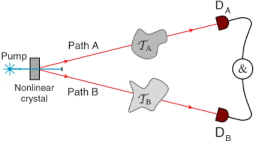
Let us consider a typical SPDC setup where pairs of pho-tons are created in the quantum state␳ along two well de-fined spatial modes共say, pathA and pathB兲 of the electro-magnetic field, as shown in Fig.1. Each photon of the pair encodes a polarization qubit and ␳ can be represented by a 4⫻4 Hermitean matrix. LetTAandTBbe two distinct optical devices put across path A and path B, respectively. Their action upon the two-qubit state␳can be described by a bilo-cal quantum map␳→EA丢EB关␳兴 关39兴. A subclass of bilocal quantum maps occurs when eitherTA orTB is not present in the setup, then eitherEA=I or EB=I, respectively, and the corresponding map is said to be local. In the above expres-sionsI represents the identity map: It does not change any input state. When a map is local, that is when it acts on a single qubit, it is subjected to some restrictions. This can be easily understood in the following way: For definiteness, let assume EB=I so that the local map E can be written as E关␳兴=EA丢I关␳兴. Let Alice and Bob be two spatially sepa-rated observer who can detect qubits in modes A and B, respectively, and let␳ and␳_Edenote the two-qubit quantum state before and after TA, respectively. In absence of any causal connection between photons in pathAwith photons in pathB, special relativity demands that Bob cannot detect via any type of local measurement the presence of the deviceTA located in pathA. Since the state of each qubit received by Bob is represented by the reduced density matrix ␳_EB

TB Path B

Path A

B D

Nonlinear crystal

A D

&

TA Pump

FIG. 1. 共Color online兲Layout of a typical SPDC experimental setup. An optically pumped nonlinear crystal emits photon pairs that propagate along pathAandBthrough the scattering devicesT_Aand

=兩Tr兩A共␳_E兲, the locality constraint can be written as

␳EB=␳B. 共12兲 We can write explicitly the mapEA丢I as a Kraus operator-sum decomposition关1兴

␳哫␳E⬀

兺

␮=0 3

␭␮共A␮丢I兲␳共A␮† 丢I兲, 共13兲

where, from now on, the symbolIdenotes the 2⫻2 identity matrix and兵A_␮其is a set of four 2⫻2 Jones matrices describ-ing the action ofTA. Then, Eq.共12兲becomes

兺

_k

,l

␳li,kj

冉

兺

␮=0 3

␭␮A␮†A␮

冊

kl

⬀

兺

k

␳ki,kj, 共14兲 which implies the trace-preserving condition on the local mapEA丢I:

兺

␮=0 3

␭␮A␮†A␮⬀I. 共15兲

Local maps that do not satisfy Eq.共15兲are classified as non-physical. In this section we show how to associate a general two-qubit quantum map E关␳兴=EA丢EB关␳兴 to the classical Mueller matricesMAandMBdescribing the optical devices TA and TB, respectively. Surprisingly, we shall find that physical linear optical devices exist共dichroic elements兲that may generate nonphysical two-qubit quantum maps关40兴.

Let denotes with 兩ij典⬅兩i典丢兩j典,i,j僆兵0 , 1其 the two-qubit standard basis. A pair of qubits is initially prepared in the generic state ␳=␳ij,kl兩ij典具kl兩=␳ik,jl

R _兩

i典具k兩丢兩j典具l兩, where super-script R indicates reshuffling 关34兴 of the indices, the same operation we used to pass from M to H: ␳ik,jl

R _⬅␳ ij,kl =具ij兩␳兩kl典. ␳ is transformed under the action of the bilocal linear mapE关␳兴=EA丢EB关␳兴into the state

␳E=EA丢EB关␳兴⬀

兺

␮,␯ ␭_␮A_␭

␯

B_共

A_␮丢B_␯兲␳共A†_␮丢B_␯†兲, 共16兲 where 兵A_␮其 and 兵B_␯其 are two sets of 2⫻2 Jones matrices describing the action of TA and TB, respectively. From Eq.

共16兲 we can calculate explicitly the matrix elements

具ij兩␳_E兩kl典=共␳_E兲ij,klin the two-qubit standard basis

共␳E兲ij,kl⬀ ␭_␮ A_共

A_␮兲im共A_␮ⴱ兲kp␳mp,nq R _␭

␯

B_共

B_␯兲jn共B_␯ⴱ兲lq

=Mik_,mp A _Mjl

,nq B

␳mp,nq R

, 共17兲

where summation over repeated Latin and Greek indices is understood. Since by definition共␳_E兲ij,kl=共␳_ER兲ik,jl we can re-write Eq.共17兲using only Greek indices as

共␳ER兲␣␤⬀M␣␮A M␤␯B ␳␮␯R =共MA丢MB兲␣␤,␮␯␳␮␯

R

, 共18兲 where summation over repeated Greek indices is again un-derstood. Equation共18兲 relates classical quantities 共the two Mueller matricesMA andMB兲with quantum ones 共the in-put and outin-put density matrices␳R_and␳

E

R

, respectively兲, thus realizing the sought connection between classical polariza-tion optics and two-qubit quantum maps.

An important case occurs whenEB=I⇒MB_=I

4 and Eq. 共18兲reduces to

␳ER⬀MA␳R. 共19兲 Equation共19兲illustrates once more the simple relation exist-ing between theclassical Mueller matrixMA_{and the} quan-tum state␳_E.

With a typical SPDC setup it is not difficult to prepare pairs of entangled photons in the singlet polarization state. Via a direct calculation, it is simple to show that when ␳ represents two qubits in the singlet state ␳s=

1

4共␴0丢␴0−␴1

丢␴1−␴2丢␴2−␴3丢␴3兲 and MA is normalized in such a

way thatM₀₀A = 1, then the proportionably symbol in the last equation above can be substituted with the equality symbol:

␳ER=M␳s R_⇒

␳E=共M␳s R_兲R

, 共20兲

where, from now on, we write M for MA _{to simplify the} notation. Note that this pleasant property is true not only or the singlet but for all four Bell states关1兴, as well. Equation

共20兲 has several remarkable consequences: Let M denotes the real-valued Mueller matrix associated toMand assume M00= 1. Then, the following results hold:

Tr共␳_E2兲= Tr共MMT兲/4, 共21兲

兩Tr兩A共␳˜E兲=共A+D兲+M01共B+C兲+iM02共B−C兲

+M03共A−D兲, 共22兲

where˜␳_E⬅共M␳R_兲R

is the un-normalized output density ma-trix. Equation 共22兲 is more general than Eq. 共21兲, since it holds for any input density matrix ␳ and not only for the singlet one ␳s. In addition, in Eq. 共22兲 we wrote the input density matrix␳ in a block-matrix form as

␳=

冋

A B

C D

册

, 共23兲

whereA, B, C=B†_{, andD are 2⫻2 submatrices and A+D}

=兩Tr兩A共␳兲. Equation共21兲shows that the degree of mixedness of the quantum state ␳_E is in a one-to-one correspondence with the classical depolarizing power关25兴of the device rep-resented byM. Finally, Eq. 共22兲, together with Eqs.共5兲and

共12兲, tells us that the two-qubit quantum map Eq. 共20兲 is trace preserving only if the device is not dichroic, namely, only ifdT_=共M

01,M02,M03兲=共0 , 0 , 0兲. This last result shows

that despite of their physical nature 共think of, e.g., a polar-izer兲, dichroic optical elements must be handled with care when used to build two-qubit quantum maps. We shall dis-cuss further this point in the next section.

Before concluding this section, we want to point out the analogy between the 16⫻16 Mueller matrix M=MA

丢MB

associated to a bilocal two-qubit quantum map, and the 4⫻4 Mueller-Jones matrix M=T丢Tⴱ representing a nondepolarizing device in a one-qubit quantum map. In both cases the Mueller matrix is said to be separable. Then, in Eq.

M=

兺

A,B

wABMA丢MB

, 共24兲

where wABⱖ0, wAB⫽wA⫻wB, and indices A, B run over two ensembles of arbitrary Mueller matrices MA _{and M}B representing optical devices located in path A and path B, respectively.

V. APPLICATIONS

In this section we exploit our formalism, by applying it to two different cases. As a first application, we build a simple phenomenological model capable to explain certain of our recent experimental results关21兴about scattering of entangled photons. The second application consists in the explicit con-struction of a bilocal quantum map generating two-qubit MEMS states. A realistic physical implementation of such map is also given.

A. Example 1: Simple phenomenological model

In Ref.关21兴, by using a setup similar to the one shown in Fig. 1, we have experimentally generated entangled two-qubit mixed states that lie upon and below the Werner curve in the linear entropy-tangle plane关41兴. In particular, we have found the following.共a兲Birefringent scatterers always pro-duce generalized Werner states of the form␳GW=V丢I␳WV†

丢I, where ␳W denotes ordinary Werner states 关42兴 and V represents an arbitrary unitary operation.共b兲 Dichroic scat-terers generate sub-Werner states, that is states that lie below the Werner curve in the linear entropy-tangle plane. In both cases, the input photon pairs were experimentally prepared in the polarization singlet state␳s. In this subsection we build, with the aid of Eq.共20兲, a phenomenological model explain-ing both results共a兲and共b兲.

To this end let us consider the experimental setup repre-sented in Fig.1. According to the actual scheme used in Ref.

关21兴, where a single scattering device was present, in this subsection we assume TB=I, so that the resulting quantum map is local. The scattering elementTA inserted across path Acan be classically described by some Mueller matrix M. In Ref. 关26兴, Lu and Chipman have shown that any given Mueller matrixMcan be decomposed in the product

M=MDMBM_⌬, 共25兲

whereM_⌬,MB, and MDare complex-valued Mueller ma-trices representing a pure depolarizer, a retarder, and a diat-tenuator, respectively. Such decomposition is not unique, for example, M=M_⌬MDMB is another valid decomposition

关43兴. Of course, the actual values of M_⌬, MB, and MD depend on the specific order one chooses. However, in any case they have the general forms given below:

M⌬=

冤

1 +c

2 0 0

1 −c 2

0 a+b 2

a−b

2 0

0 a−b 2

a+b

2 0

1 −c

2 0 0

1 +c 2

冥

, 共26兲

MB=TU丢TUⴱ, 共27兲

MD=TH丢THⴱ, 共28兲

wherea,b,c僆R andTU,THare the unitary and Hermitean Jones matrices representing a retarder and a diattenuator, re-spectively. Actually, the expression ofM_⌬given in Eq.共26兲 is not the most general possible关26兴, but it is the correct one for the representation of pure depolarizers with zero polari-zance, such as the ones used in Ref.关21兴. Note that although MBandMDare Mueller-Jones matrices,M_⌬is not. When a=b=c⬅p:p僆关0 , 1兴 the depolarizer is said to be isotropic

共or, better, polarization isotropic兲. This case is particularly relevant when birefringence and dichroism are absent. In this case MB=I₄=MD, and Eq. 共25兲 gives M=M_⌬. Thus, by using Eq.共26兲we can calculateM_⌬共p兲and use it in Eq.共20兲 to obtain

␳E=p␳s+ 1 −p

4 I4⬅␳W, 共29兲 that is, we have just obtained a Werner state:␳_E=␳W. Thus, we have found that a local polarization-isotropic scatterer acting upon the two-qubit singlet state, generates Werner states.

Next, let us consider the cases of birefringent共retarders兲 and dichroic 共diattenuators兲 scattering devices that we used in our experiments. In these cases the total Mueller matrices Mof the devices under consideration can be written asM =MZM_⌬, where eitherZ=BorZ=D, andM_⌬=M_⌬共p兲 rep-resents a polarization-isotropic depolarizer. For definiteness, let consider in detail only the case of a birefringent scatterer, since the case of a dichroic one can be treated in the same way. In this case

MBM_⌬共p兲=

兺

␮=0 3

␭␮共p兲TUT␮丢TUⴱT␮ⴱ 共30兲

and, as result of a straightforward calculation, ␭₀=共1 + 3p兲/ 2, ␭1=␭2=␭3=共1 −p兲/ 2, T␮=X␮/

冑

2; while TU is an arbitrary unitary 2⫻2 Jones matrix representing a generic retarder. For the sake of clarity, instead of using directly Eq.

共20兲, we prefer to rewrite Eq.共16兲adapted to this case as

␳E=

兺

␮=0 3

␭␮共p兲共TUT␮丢I兲␳s共T_␮†TU

†

丢I兲

=TU丢I

冋

兺

␮=0 3

␭␮共p兲共T␮丢I兲␳s共T_␮† 丢I兲

册

TU

†

丢I

=TU丢I␳WT†U丢I=␳GW, 共31兲

where Eq. 共29兲has been used. Equation 共31兲clearly shows that the effect of a birefringent scatterer is to generate what we called generalized Werner states, in full agreement with our experimental results关21兴.

␳E⬀˜␳E=TH丢I␳WTH

†

丢I, 共32兲

whereTHis a 2⫻2 Hermitean matrix representing a generic diattenuator关19兴

TH=

冋

d0cos␪2+d1sin␪2 共d0−d1兲cos␪sin␪ 共d0−d1兲cos␪sin␪ d1cos␪2+d0sin␪2

册

,

共33兲

where di僆关0 , 1兴 are the diattenuation factors, while

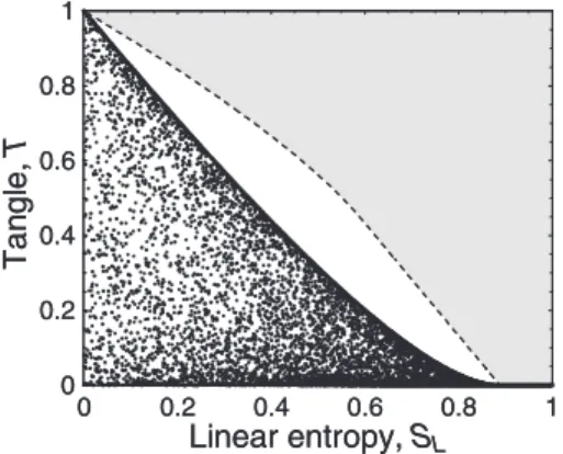
␪僆共0 , 2␲兴gives the direction of the transmission axis of the linear polarizer to which TH reduces when either d0= 0 or d1= 0. Figure2reports, in the linear entropy-tangle plane, the

results of a numerical simulation were we generated 104

states ␳_E from Eq. 共32兲, by randomly generating共with uni-form distributions兲the four parametersp,d0,d1, and␪in the

ranges p,d0,d1僆关0 , 1兴, ␪僆共0 , 2␲兴. The numerical

simula-tion shows that a local dichroic scatterer may generate sub-Werner two-qubit states, that is, states located below the Werner curve in the linear entropy-tangle plane. The qualita-tive agreement between the result of this simulation and the experimental findings shown in Fig. 3 of Ref.关21兴is evident. Discussion. It should be noticed that while we used the equality symbol in writing Eq.共31兲, we had to use the pro-portionality symbol in writing Eq. 共32兲. This is a conse-quence of the Hermitean character of the Jones matrix TH that generates a non-trace-preserving map. In fact, in this case from M=MDM⌬共p兲, where MD=共VTH丢THⴱV†兲/ 2 and

M_⌬共p兲=关VM_⌬共p兲V†兴/ 2, we obtain Tr共˜␳_E兲=共d2₀+d₁2兲/ 2⫽1. Moreover, Eq.共22兲gives

␳EB=兩Tr兩A共␳E兲=

X0

2 −p

冉

d₀2−d₁2 d₀2+d₁2

冊

X1sin 2␪+X3cos 2␪

2 ,

共34兲

where␳_E=˜␳_E/ Tr共˜␳_E兲. This result is in contradiction, for d0 ⫽d1, with the locality constraint expressed by Eq. 共12兲

which requires

␳EB= X0

2 . 共35兲

As we already discussed in the previous section, only the latter result seems to be physically meaningful since photons in path B, described by ␳_EB, cannot carry information about device TA which is located across path A. On the contrary, Eq. 共34兲 shows that ␳_EB is expressed in terms of the four physical parametersp,d0,d1, and␪ that characterizeTA. Is

there a contradiction here?

In fact, there is not. One should keep in mind that Eq.共34兲 expresses the one-qubit reduced density matrix ␳_EB that is extracted from the two-qubit density matrix␳_Eafter the latter has been reconstructed by the two observers Alice and Bob by means of nonlocal coincidence measurements. Such ma-trix contains information about both qubits and, therefore, contains also information aboutTA. Conversely,␳_EB=X0/ 2 in

Eq.共35兲, is the reduced density matrix that could be recon-structed by Bob alone via local measurements before he and Alice had compared their own experimental results and had selected from the raw data the coincidence counts.

From a physical point of view, the discrepancy between Eqs.共34兲and共35兲is due to the polarization-dependent losses

共that is, d₀⫽d1兲 that characterize dichroic optical devices and it is unavoidable when such elements are present in an experimental setup. Actually, it has been already noticed that a dichroic optical element necessarily performs a kind of post-selective measurement 关16兴. In our case coincidence measurements post-select only those photons that have not been absorbed by the dichroic elements present in the setup. However, since in any SPDC setup even the initial singlet state is actually a post-selected state共in order to cut off the otherwise overwhelming vacuum contribution兲, the practical use of dichroic devices does not represent a severe limitation for such setups.

B. Example 2: Generation of two-qubit MEMS states

In the previous subsection we have shown that it is pos-sible to generate two-qubit states represented by points upon and below the Werner curve in the linear entropy-tangle plane, by operating on a single qubit 共local operations兲 be-longing to a pair initially prepared in the entangled singlet state. In another paper 关40兴 we have shown that it is also possible to generate MEMS states共see, e.g., Refs. 关41,44兴, and references therein兲, via local operations. However, the price to pay in that case was the necessity to use a dichroic device that could not be represented by a “physical,” namely, a trace-preserving, quantum map. In the present subsection, as an example illustrating the usefulness of our conceptual scheme, we show that by allowing bilocal operations per-formed by two separate optical devicesTAandTBlocated as in Fig.1, it is possible to achieve MEMS states without using dichroic devices.

To this end, let us start by rewriting explicitly Eq.共16兲, where the most general bilocal quantum map E关␳兴=EA

丢EB关␳兴operating upon the generic input two-qubit state␳, is represented by a Kraus decomposition

0 0.2 0.4 0.6 0.8 1

Linear entropy,SL

0 0.2 0.4 0.6 0.8 1

el

g

n

a

T,

T

0 0.2 0.4 0.6 0.8 1

Linear entropy,SL

0 0.2 0.4 0.6 0.8 1

el

g

n

a

T,

T

␳E=EA丢EB关␳兴=

兺

␮,␯␭␮

A_␭

␯

B_共

A_␮丢B_␯兲␳共A†_␮丢B_␯†兲, 共36兲 where now the equality symbol can be used since we assume that both single-qubit mapsEAandEB are trace preserving

兺

␮=0 3

␭_␮A

A_␮†A_␮=I=

兺

␯=0 3

␭_␯B

B_␯†B_␯ 共37兲

but not necessarily unital: EF关I兴⫽I,F僆兵A,B其 关39兴. Under the action ofE, the initial state of each qubit traveling in path Aor pathB is transformed into either the output state

␳EA=兩Tr兩B共␳_E兲=

兺

␮=0 3

␭_␮A

A_␮␳AA_␮† 共38兲 or

␳EB=兩Tr兩A共␳_E兲=

兺

␯=0 3

␭_␯B

B_␯␳BB_␯†, 共39兲 respectively, where ␳A=兩Tr兩B共␳兲 and ␳B=兩Tr兩A共␳兲. Without loss of generality, we assume that the two qubits are initially prepared in the singlet state␳=␳s. Then Eqs.共38兲 and共39兲 reduce to ␳_EF_=兺

␣␭␣FF␣F␣†/ 2, F僆兵A,B其. From the previous

analysis 关see Eqs. 共16兲–共18兲兴 we know that to each bilocal quantum map EA丢EB can be associated a pair of classical Mueller matricesMA andMB such that

共␳ER兲␣␤=

兺

␮,␯

共MA

丢MB_兲

␣␤,␮␯共␳s R_兲

␮␯. 共40兲

The real-valued Mueller matrices MA _{and M}B _{associated to} MA_andMB_{, respectively, can be written as}

MA=

冋

1 0 T

a A

册

, M

B

=

冋

1 0 T

b B

册

, 共41兲 where Eq.共5兲withdA=0=dBandM00= 1 has been used, and

pA⬅a=

冤

a1 a2 a3

冥

, pB⬅b=

冤

b1 b2 b3

冥

, 共42兲

are the polarizance vectors ofMA _andMB_{, respectively. We} remember that the conditiondA=dB=0 is a consequence of the fact that both mapsEAandEBare trace preserving, while the conditionsa⫽0andb⫽0reflect the nonunital nature of EA andEB. With this notation we can rewrite Eqs.共38兲and

共39兲as

␳EA= 1 2_␮

兺

₌₀

3

a_␮X_␮, 共43兲

␳EB= 1 2

兺

_␯=0

3

b_␯X_␯, 共44兲

where we have defineda₀= 1 =b₀. Moreover, the output two-qubit density matrix␳_E=E关␳s兴can be decomposed into a real and an imaginary part as␳_E=␳_ERe+i␳_EIm, where

␳ERe= 1 4

冤

␣+ + _␤

+ ␥+ ␦+

␤+ ␣−+ ␦− ␥−

␥+ ␦− ␣+ − _␤

−

␦+ ␥− ␤− ␣−−

冥

共45兲

and

␳EIm= 1 4

冤

0 −␰+ −␩+ −␶+

␰+ 0 −␶− −␩−

␩+ ␶− 0 −␰−

␶+ ␩− ␰− 0

冥

共46兲

with

␣±+⬅ 共1 +a3兲±关b3共1 +a3兲−C33兴,

␣±−⬅ 共1 −a3兲±关b3共1 −a3兲+C33兴, 共47兲

and

␤±⬅b1±共a3b1−C31兲, ␥±⬅a1±共a1b3−C13兲,

␦±⬅a1b1−C11⫿共a2b2−C22兲, 共48兲

and

␰±⬅b2±共a3b2−C32兲, ␩±⬅a2±共a2b3−C23兲,

␶±⬅a2b1−C21±共a1b2−C12兲, 共49兲

whereCij⬅共ABT兲ij,i,j僆兵1 , 2 , 3其.

At this point, our goal is to determine the two vectorsa,b

and the two 3⫻3 matrices A,Bsuch that␳_EIm= 0 and

␳ERe=␳MEMS=

冤

g共p兲/2 0 0 p/2 0 1 −g共p兲 0 0

0 0 0 0

p/2 0 0 g共p兲/2

冥

, 共50兲

where

g共p兲=

再

2/3, 0ⱕpⱕ2/3,

p, 2/3⬍pⱕ1.

冎

共51兲 To this end, first we calculatea andb by imposing

␳EA=␳MEMS

A

=

冋

1 −g共p兲/2 0

0 g共p兲/2

册

, 共52兲

␳EB=␳MEMS

B

=

冋

g共p兲/2 0

0 1 −g共p兲/2

册

, 共53兲 respectively. Note that only fulfilling Eqs.共52兲and共53兲, to-gether with␳_ERe=␳MEMSand␳EIm= 0, will ensure the achieve-ment of true MEMS states. It is surprising that in the current literature the importance of this point is neglected. Thus, by solving Eqs.共52兲and共53兲we obtaina1=a2= 0,a3= 1 −g共p兲,

共41兲in terms of the two real-valued Mueller matrices

MA=

冤

1 0 0 0

0

冑

p 0 0

0 0

冑

p 0

1 −g共p兲 0 0 g共p兲

冥

,

MB₌

冤

1 0 0 0

0 −

冑

p 0 0

0 0

冑

p 0

g共p兲− 1 0 0 −g共p兲

冥

. 共54兲

It is easy to check that both MA _andMB _{are physically} ad-missible Mueller matrices since the associated matricesHA andHBhave the same spectrum made of non-negative eigen-values兵␭_␮A其=兵␭_␮B其⬅兵␭_␮其=兵␭0,␭1,␭2,␭3其. In particular:

兵␭␮其=兵0, 1 −p, 0, 1 +p其, for 2/3⬍pⱕ1 共55兲

and

兵␭␮其=

再

0,1

3,

5 −

冑

1 + 36p

6 ,

5 +

冑

1 + 36p

6

冎

共56兲

for 0ⱕpⱕ2 / 3. It is also easy to see that the mapE can be decomposed as in Eq.共36兲in a Kraus sum withA0=A2= 0

A1

冑

␭1=

冋

0

冑

1 −p

0 0

册

, A3

冑

␭3=

冋

1 0

0

冑

p

册

共57兲 andB₀=B₂= 0

B₁

冑

␭₁=

冋

0 0

0

冑

1 −p

册

, B3

冑

␭3=

冋

0 −

冑

p

1 0

册

共58兲 for 2 / 3⬍pⱕ1. Analogously, for 0ⱕpⱕ2 / 3 we have A0

= 0

A1

冑

␭1=

冋

0 1/

冑

3

0 0

册

, 共59兲

A2

冑

␭2=

冋

−␾₋ 0 0 ␺+

册

, A3

冑

␭3=

冋

␾+ 0

0 ␺−

册

共60兲

andB0= 0

B₁

冑

␭₁=

冋

0 0

0 1/

冑

3

册

, 共61兲

B2

冑

␭2=

冋

0 ␺+

␾− 0

册

, B3

冑

␭3=

冋

0 −␺−

␾+ 0

册

, 共62兲

where

␾±⬅

冑

1 2

冉

1 ±

1 + 6p

冑

1 + 36p

冊

, 共63兲

␺±⬅

冑

1 3

冉

1 ±

1 − 9p

冑

1 + 36p

冊

. 共64兲 Note that these coefficients satisfy the following relations:

␾+ 2

+␾₋2= 1, 共65兲

1

3+␺+2+␺−2= 1. 共66兲

A straightforward calculation shows that the single-qubit mapsEA andEBare trace-preserving but not unital, since

兺

␮=0 3

␭␮A␮A␮†=

冋

2 −g共p兲 0

0 g共p兲

册

共67兲

and

兺

␯=0 3

␭_␯B_␯B_␯†=

冋

g共p兲 0

0 2 −g共p兲

册

. 共68兲

At this point our task has been fully accomplished. How-ever, before concluding this subsection, we want to point out that both mapsEA andEB must depend on the same param-eterp in order to generate proper MEMS states. This means that either a classical communication must be established betweenTA and TB in order to fix the same value of p for both devices or a classical signal encoding the information about the value ofp must be sent toward both TA andTB.

Physical implementation. Now we furnish a straightfor-ward physical implementation for the quantum maps pre-sented above. Up to now, several linear optical schemes gen-erating MEMS states were proposed and experimentally tested. Kwiat and co-workers 关41兴were the first to achieve MEMS using photon pairs from spontaneous parametric down conversion. Basically, they induced decoherence in SPDC pairs initially prepared in a pure entangled state by coupling polarization and frequency degrees of freedom of the photons. At the same time, a somewhat different scheme was used by De Martini and co-workers 关44兴 who instead used the spatial degrees of freedom of SPDC photons to induce decoherence. In such a scheme the use of spatial de-grees of freedom of photons required the manipulation of not only the emitted SPDC photons, but also of the pump beam. In this subsection, we show that both single-qubit maps EA andEB can be physically implemented as linear optical networks 关6兴 where polarization and spatial modes of pho-tons are suitably coupled, without acting upon the pump beam. The basic building blocks of such networks are polar-izing beam splitters 共PBSs兲, half-waveplates 共HWPs兲, and mirrors. Let兩i,N典be a single-photon basis, where the indices i andN label polarization and spatial modes of the electro-magnetic field, respectively. We can also write兩i,N典=aˆiN

†_兩

0典 in terms of the annihilation operators aˆiN and the vacuum state 兩0典. A polarizing beam splitter distributes horizontal 共i =H兲and vertical共i=V兲polarization modes over two distinct spatial modes, sayN=n andN=m, as follows:

兩H,n典in→兩H,n典out and 兩V,n典in→兩V,m典out,

兩H,m典in→兩H,m典out and 兩V,m典in→兩V,n典out, 共69兲

THWP共␪兲=

冋

− cos 2␪ − sin 2␪

− sin 2␪ cos 2␪

册

, 共70兲 where␪is the angle the optic axis makes with the horizontal polarization. Two half-waveplates in series constitute a po-larization rotator represented by TR共␪兲=THWP共␪0

+␪/ 2兲THWP共␪0兲, where ␪0 is an arbitrary angle and TR共␪兲=

冋

cos␪ − sin␪

sin␪ cos␪

册

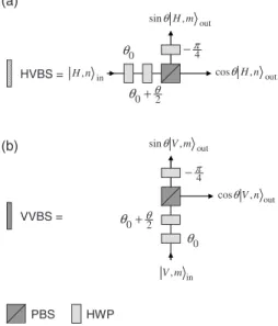
. 共71兲

By combining these basic elements, composite devices may be built. Figures4共a兲and4共b兲 show the structure of a horizontal共a兲and vertical共b兲variable beam splitter, denoted HVBS and VVBS, respectively. HVBS performs the follow-ing transformation

兩H,n典in→cos␪兩H,n典out+ sin␪兩H,m典out, 共72兲 while VVBS makes

兩V,m典in→cos␪兩V,n典out+ sin␪兩V,m典out. 共73兲 At this point we have all the ingredients necessary to built the optical linear networks corresponding to our maps. We begin by illustrating in detail the optical network

implement-ingEA 共for 2 / 3⬍pⱕ1兲, which is shown in Fig.5. Let兩␺0典 =a兩H典+b兩V典 be the input single-photon state entering the network. If we define the VVBS angle

␪p= arccos

冑

p, 共74兲 then it is easy to obtain after a straightforward calculation:

兩␣1

I_典

=

冑

␭1A1兩␺0典=b

冑

1 −p兩H典, 共75兲 兩␣3

I_典

=

冑

␭₃A3兩␺0典=a兩H典+b

冑

p兩V典. 共76兲 Since detectorDA does not distinguish spatial mode 1 from spatial mode 2, the two states兩␣₁I典and兩␣₃I典, sum incoherently and the single-photon output density matrix can be written as

␳EA=兩␣1

I_典具␣

1

I_兩

+兩␣₃I典具␣₃I兩, where

␳EA=

冋

兩a兩2+兩b兩2共1 −p兲 abⴱ

冑

p

aⴱb

冑

p p兩b兩2

册

. 共77兲 Of course, if we write the input density matrix as ␳₀ =兩␺0典具␺0兩, it is easy to see that

␳EA=

兺

␮=0 3

␭␮A␮␳0A␮†, 共78兲

where Eq.共57兲 has been used. Equation共78兲, together with Eq.共38兲, proves the equivalence between the quantum map EAand the linear optical setup shown in Fig.5. Note that the Mach-Zehnder interferometers present in Figs. 5 and 6 are balanced, that is, their arms have the same optical length. In a similar manner, we can physically implementEB 共for 2 / 3 ⬍pⱕ1兲, in the optical network shown in Fig. 6, where we have defined

in ,n

i i,n_out

out ,m j

in ,m j

FIG. 3. The polarizing beam splitter couples horizontal and ver-tical polarization modes 共i,j僆兵H,V其兲, with two distinct spatial modesN=nandN=mof the electromagnetic field.

0

θ

2 0 θ

θ +

0

θ

2 0 θ

θ + in

,n H

4

π

−

out

, cosθHn out

, sinθHm

4

π

−

in

,m V

out

, cosθVn out

, sinθVm

PBS HWP

HVBS =

VVBS =

(a)

(b)

FIG. 4. The variable beam splitters HVBS and VVBS.

o

45

o

0

PBS HWP

VVBS Mirror

p

θ

H

V

0

ψ

A

D I 1

α

I

3

α

FIG. 5. Linear optical network implementing E_A 共for 2 / 3⬍p

兩␤1

I_典

=

冑

␭1B1兩␺0典=b

冑

1 −p兩V典, 共79兲 兩␤3

I_典

=

冑

␭₃B₃兩␺₀典= −b

冑

p兩H典+a兩V典, 共80兲 and, again,␳_EB=兩␤₁I典具␤₁I兩+兩␤₃I典具␤₃I兩.

The optical networks necessary to realize quantum maps generating MEMS II states are a bit more complicated. In

order to illustrate them we need to define the following two angles␪_1/3and␪_␺that determine the transmission amplitudes of two VVBSs used in the MEMS II networks:

␪1/3= arccos

冑

1

3, 共81兲

␪␺= arccos

冉

冑

3

2␺+

冊

. 共82兲

In addition, a third angle ␪_␾ determining the transmission amplitudes of a HVBS, must be introduced:

␪␾= arccos␾+. 共83兲

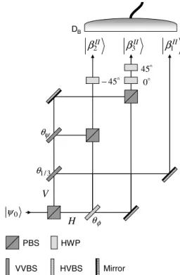
Then, the mapEA共for 0ⱕpⱕ2 / 3兲, is realized by the optical network shown in Fig.7, where we have defined

兩␣2II典=

冑

␭2A2兩␺0典= −a␾−兩H典+b␺+兩V典, 共84兲 兩␣3II典=

冑

␭3A3兩␺0典=a␾+兩H典+b␺−兩V典, 共85兲

兩␣1 II_典

=

冑

␭1A1兩␺0典= b

冑

3兩H典. 共86兲 In this case, incoherent detection produces the output mixed state ␳_E

A=兩␣2 II_典具␣

2 II_兩

+兩␣₃II典具␣₃II兩+兩␣₁II典具␣₁II兩. Finally, the mapEB

共for 0ⱕpⱕ2 / 3兲, is realized by the optical network shown in Fig.8, where we have defined

兩␤2II典=

冑

␭2B2兩␺0典=b␺+兩H典+a␾−兩V典, 共87兲

PBS HWP

VVBS Mirror

0

45

p θ

H

V

0 ψ

B D

I 1

β

I

3

β

FIG. 6. Linear optical network implementing E_B 共for 2 / 3⬍p

ⱕ1兲, for MEMS I generation.

A

D

o

0

ψ

θ

φ

θ

H

II

2

α II

3

α II

1 α

V

0

ψ

PBS HWP

VVBS HVBS Mirror

3 / 1

θ

o

0

o

45

FIG. 7. Linear optical network implementing EA 共for 0ⱕp ⱕ2 / 3兲, for MEMS II generation. Each of the two Mach-Zehnder interferometers constituting the network are balanced.

B

D

o

45

− 0o

o

45

ψ θ

φ θ

H II 2

β II

3

β II

1 β

V

0

ψ

PBS HWP

VVBS HVBS Mirror

3 / 1

θ

FIG. 8. Linear optical network implementing E_B 共for 0ⱕp

兩␤3 II_典

=

冑

␭3B3兩␺0典= −b␺−兩H典+a␾+兩V典, 共88兲 兩␤1II典=

冑

␭1B1兩␺0典=

b

冑

3兩V典. 共89兲 As before, now we have␳_E

B=兩␤2 II_典具␤

2 II_兩+兩␤

3 II_典具␤

3 II_兩+兩␤

1 II_典具␤

1 II_兩.

VI. SUMMARY AND CONCLUSIONS

Classical polarization optics and quantum mechanics of two-level systems are two different branches of physics that share the same mathematical machinery. In this paper we have described the analogies and connections between these two subjects. In particular, after a review of the matrix for-malism of classical polarization optics, we established the

exact relation between one- and two-qubit quantum maps and classical description of linear optical processes. Finally, we successfully applied the formalism just developed, to two cases of practical utility.

We believe that the present paper will be useful to both the classical and the quantum optics community since it en-lightens and puts on a rigorous basis, the so-widely used relations between classical polarization optics and quantum mechanics of qubits. A particularly interesting aspect of our work is that we describe in detail how dichroic devices共i.e., devices with polarization-dependent losses兲, fit into this gen-eral scheme.

ACKNOWLEDGMENT

This project was supported by FOM.

关1兴M. A. Nielsen and I. L. Chuang,Quantum Computation and Quantum Information, reprinted 1st ed.共Cambridge University Press, Cambridge, UK, 2002兲

关2兴A. Zeilinger, Rev. Mod. Phys. 71, S288共1999兲.

关3兴N. Gisin, G. Ribody, W. Tittel, and H. Zbinden, Rev. Mod. Phys. 74, 145共2002兲.

关4兴E. Knill, R. Laflamme, and G. Milburn, Nature共London兲 409, 46共2001兲.

关5兴J. L. O’Brien, G. J. Pryde, A. G. White, T. C. Ralph, and D. Branning, Nature共London兲 426, 264共2003兲.

关6兴J. Skaar, J. C. G. Escartín, and H. Landro, Am. J. Phys. 72, 1385共2004兲.

关7兴P. Kok, W. J. Munro, K. Nemoto, T. C. Ralph, J. P. Dowling, and G. J. Miburn, Rev. Mod. Phys. 79, 135共2007兲, and refer-ences therein.

关8兴D. Bouwmeester, J. W. Pan, K. Mattle, M. Eibl, H. Weinfurter, and A. Zeilinger, Nature共London兲 390, 575共1997兲.

关9兴D. Boschi, S. Branca, F. De Martini, L. Hardy, and S. Popescu, Phys. Rev. Lett. 80, 1121共1998兲.

关10兴D. F. V. James, P. G. Kwiat, W. J. Munro, and A. G. White, Phys. Rev. A 64, 052312共2001兲.

关11兴J. L. O’Brien, G. J. Pryde, A. Gilchrist, D. F. V. James, N. K. Langford, T. C. Ralph, and A. G. White, Phys. Rev. Lett. 93, 080502共2004兲.

关12兴N. Peters, J. Altepeter, E. Jeffrey, D. A. Branning, and P. Kwiat, Quantum Inf. Comput. 3, 503共2003兲.

关13兴T.-C. Wei, J. B. Altepeter, D. Branning, P. M. Goldbart, D. F. V. James, E. Jeffrey, P. G. Kwiat, S. Mukhopadhyay, and N. A. Peters, Phys. Rev. A 71, 032329共2005兲.

关14兴A. Yariv, Quantum Electronics, 3rd ed. 共Wiley, New York, 1989兲.

关15兴C. Zhang, Phys. Rev. A 69, 014304共2004兲.

关16兴N. Brunner, A. Acín, D. Collins, N. Gisin, and V. Scarani, Phys. Rev. Lett. 91, 180402共2003兲.

关17兴A. Aiello, G. Puentes, D. Voigt, and J. P. Woerdman, Opt. Lett.

31, 817共2006兲.

关18兴M. Born and E. Wolf,Principles of Optics, 7th ed.共Cambridge University Press, Cambridge, 1999兲.

关19兴J. N. Damask, Polarization Optics in Telecommunications

共Springer, New York, 2005兲.

关20兴U. Leonhardt, Rep. Prog. Phys. 66, 1207共2003兲.

关21兴G. Puentes, D. Voigt, A. Aiello, and J. P. Woerdman, e-print arXiv:quant-ph/0607014.

关22兴D. L. Falkoff and J. E. McDonald, J. Opt. Soc. Am. 41, 862

共1951兲; U. Fano, Phys. Rev. 93, 121共1954兲.

关23兴J. J. Sakurai, Modern Quantum Mechanics 共Benjamin/ Cummings, Menlo Park, California, 1985兲.

关24兴Actually, our Stokes parameterss_␣differ from the traditional onesS_␣as given, e.g., in Chap. 10 of关18兴. However, the two sets of parameters are related by the simple relationsS0=s0, S₁=s₃,S₂=s₁,S₃= −s₂.

关25兴F. Le Roy-Brehonnet and B. L. Jeune, Prog. Quantum Elec-tron. 21, 109共1997兲.

关26兴S.-Y. Lu and R. A. Chipman, J. Opt. Soc. Am. A 13, 1106

共1996兲.

关27兴A. Fujiwara and P. Algoet, Phys. Rev. A 59, 3290共1999兲.

关28兴A. Aiello and J. P. Woerdman, e-print arXiv:math-ph/0412061.

关29兴J. J. Gil, J. Opt. Soc. Am. A 17, 328共2000兲.

关30兴K. Kim, L. Mandel, and E. Wolf, J. Opt. Soc. Am. A 4, 433

共1987兲.

关31兴M. B. Ruskai, S. Szarek, and E. Werner, Linear Algebr. Appl.

347, 159共2002兲.

关32兴D. G. M. Anderson and R. Barakat, J. Opt. Soc. Am. A 11, 2305共1994兲.

关33兴R. Simon, Opt. Commun. 42, 293共1982兲.

关34兴I. Bengtsson and K. Życzkowski, Geometry of Quantum States: An Introduction to Quantum Entanglement共Cambridge University Press, Cambridge, 2006兲.

关35兴E. C. G. Sudarshan, P. M. Mathews, and J. Rau, Phys. Rev.

121, 920共1961兲; M.-D. Choi, Linear Algebra Appl. 10, 285

共1975兲.

关36兴S. R. Cloude, Optik 共Stuttgart兲 75, 26 共1986兲; Proc. SPIE

1166, 177共1989兲; J. Electromagn. Waves Appl.6, 947共1992兲.

关37兴We acknowledge Dr. Krzysztof Wódkiewick, who pointed out to us the importance of this point.

关38兴A. Aiello and J. P. Woerdman, Opt. Lett. 30, 1599共2005兲.

关40兴A. Aiello, G. Puentes, D. Voigt, and J. P. Woerdman, e-print arXiv:quant-ph/0603182.

关41兴N. A. Peters, J. B. Altepeter, D. A. Branning, E. R. Jeffrey, T.-C. Wei, and P. G. Kwiat, Phys. Rev. Lett. 92, 133601

共2004兲.

关42兴R. F. Werner, Phys. Rev. A 40, 4277共1989兲.

关43兴J. Morio and F. Goudail, Opt. Lett. 29, 2234共2004兲.