TRUMPET INITIAL DATA FOR HIGHLY BOOSTED BLACK HOLES AND HIGH ENERGY BINARIES
Kyle Patrick Slinker
A dissertation submitted to the faculty at the University of North Carolina at Chapel Hill in partial fulfillment of the requirements for the degree of Doctor of Philosophy in the Department of Physics and
Astronomy.
Chapel Hill 2017
ABSTRACT
Kyle Patrick Slinker: Trumpet Initial Data for Highly Boosted Black Holes and High Energy Binaries (Under the direction of Charles R. Evans)
TABLE OF CONTENTS
LIST OF TABLES . . . vii
LIST OF FIGURES . . . viii
LIST OF ABBREVIATIONS AND SYMBOLS . . . xii
1 Introduction . . . 1
1.1 Testing General Relativity Through Gravitational Wave Astronomy . . . 1
1.2 Numerical Relativity . . . 2
1.3 Project Goals . . . 4
1.4 Outline of the Remainder of the Thesis . . . 5
2 Decomposing Spacetimes and Einstein’s Equations . . . 6
2.1 ADM Formalism for Foliation and 3+1 Decomposition of Spacetime . . . 6
2.1.1 Gauge Choice . . . 15
2.2 Trumpet Spatial Slice Topology . . . 16
2.3 Conformal Transformations . . . 19
2.3.1 BSSN Equations: Conformal Rescaling of the Evolution Equations . . . 23
3 Measuring Properties of Black Holes and Spacetimes . . . 24
3.1 ADM Mass, Momentum, and Angular Momentum . . . 25
3.2 Black Hole Horizons and Quasi-Local Measures . . . 27
3.3 Newman-Penrose Formalism and the Weyl Scalars . . . 30
3.4 Gravitational Wave Content . . . 33
4 Numerical Methods and the Einstein Toolkit . . . 37
4.2 Resolving Features Efficiently: Mesh Refinement,Carpet, andPunctureTracker . . . 38
4.3 Evolution, Method of Lines,ML BSSN, andMoL. . . 41
4.4 Thorns and Methods for Initial Data . . . 43
4.4.1 Bowen-York Initial Data andTwoPunctures . . . 43
4.4.2 Successive Over-Relaxation andCT MultiLevel. . . 43
4.5 Thorns for Analysis . . . 45
4.5.1 Finding and Storing Apparent Horizons: AHFinderDirectand SphericalSurface . . 45
4.5.2 QuasiLocalMeasures,WeylScal4, andMultipole . . . 45
5 Building a Single Boosted Trumpet Black Hole . . . 46
5.1 Trumpet Coordinates for a Boosted Black Hole . . . 46
5.1.1 Review of Trumpet Slicing of a Static Black Hole . . . 46
5.1.2 Adapting Trumpet Slicing to Moving Punctures Gauge: Boosted Black Hole . . . 52
5.2 Setup for Numerical Simulations . . . 57
5.2.1 Review of Initial Data Scheme Implementation in Code . . . 57
5.2.2 Modifying the Computation of ADM Mass and Momentum for Moving Black Holes . 58 5.2.3 Interpreting Weyl Scalars for Moving, Off-Center Black Hole . . . 59
5.2.4 Using Apparent Horizon Circumferences as Measures of Horizon Distortion . . . 60
5.2.5 Simulation Gauge Conditions . . . 61
5.2.6 Bowen-York Initial Data as a Control . . . 62
5.2.7 Grid Set Up . . . 62
5.3 Resulting Properties of Boosted-Trumpet Coordinates and Improvements Compared to Bowen-York Initial Data . . . 62
5.3.1 Qualitative Description of Boosted-Trumpet Data Initially and After Evolution . . . . 62
5.3.2 Understanding Boosted Trumpet Gravitational Wave Due to Tetrad Offset and Dis-cretization . . . 64
5.3.3 Reduced Junk Gravitational Wave . . . 66
5.3.4 Increased Accuracy of Black Hole Speed . . . 67
5.4 Summary Remarks About Boosted-Trumpet Black Holes . . . 71
5.5 Code Validation . . . 72
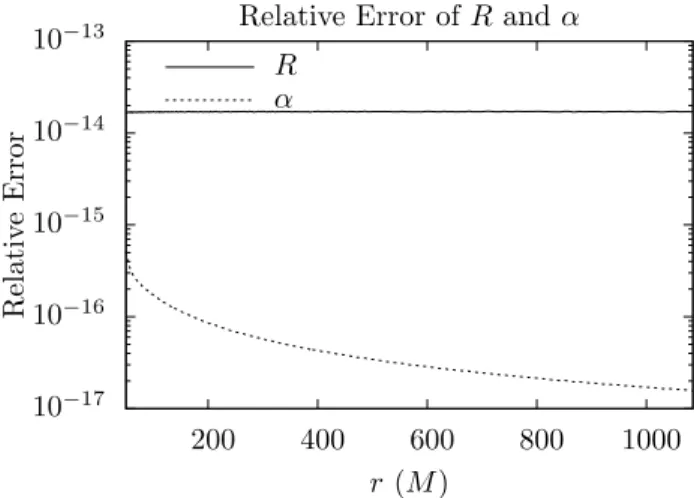
5.5.1 ADM Quantities . . . 72
5.5.2 Stationary Solution . . . 72
5.5.3 Constraint Violation . . . 73
6 Superposing Initial Data. . . 77
6.1 Recipe for Approximate (Constraint-Violating) Superposition . . . 77
6.2 Preliminary Results for a Boosted-Trumpet Binary . . . 80
7 Conclusions . . . 87
7.1 The Future of Boosted-Trumpet Initial Data . . . 87
7.1.1 Boosted-Trumpet Binaries . . . 87
7.1.2 Black Hole With Trumpet Slicing Boosted in an Arbitrary Direction . . . 87
7.1.3 Boosted-Trumpet Black Holes with Spin . . . 89
7.2 Summary Remarks . . . 90
LIST OF TABLES
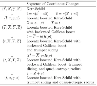
2.1 Table summarizing the information content of the the pieces of conformal transverse-traceless decomposition. . . 21 5.1 Sequence of coordinate changes described in the text. The relationship between each system
LIST OF FIGURES
2.1 The foliation of spacetime. Shown are two moments in time, Σ(t1) and Σ(t2), in the foliation,
each with its own γij and Kij. The relationship between a point xa
0 in the two members of
the foliation in terms ofαandβi also is shown. Analytically, there are an infinite number of
such slices; numerically, the code computes quantities at the two timest1andt2separated by
some small ∆t. . . 15
2.2 Embedding diagrams for the Schwarzschild spacetime. Showing level sets oft0in thet0R-plane on the left and level sets oft0 in thet0R-plane on the right (with solid lines). The singularity atR= 0 is shown with a zigzag line and the horizon at R= 2M is shown with a dashed line. The limiting radius of the trumpet slicesR=r0is shown by the dotted line in the right figure.
The flat slices (on the left) intersect the singularity after entering the horizon; in contrast, the trumpet slices (on the right) enter the horizon but limit onr0 (the dotted line) instead
of intersecting the singularity. Note that these are schematic diagrams only and were drawn without using a practical a height functionh(R). . . 18
2.3 Penrose diagrams for the Schwarzschild spacetime. Showing surfaces of constantt0 on the left and surfaces of constantt0 on the right (solid lines). The singularity atR= 0 is shown with a zigzag line and the horizon atR= 2M is shown with a dashed line. The limiting radius of the trumpet slicesR=r0 is shown by the dotted line in the right figure (these are the same
conventions used in Fig. 2.2). The flat slices (on the left) either enter the parallel universe or intersect the singularity; in contrast, the trumpet slices (on the right) enter the horizon and terminate oni+without crossingr0(the dotted line). Note that these are schematic diagrams
only and were drawn without using a practical height functionh(R). . . 18
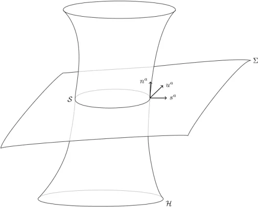
3.1 Horizon geometry. This shows the spatial slice Σ, the collection of horizons at all times H, and their intersection S = Σ∩ H. It also shows na, the normal to Σ; sa, the normal to S within Σ; andua, the outgoing null vector constructed fromna andsa and used in (3.17). . 29
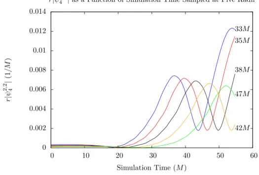
3.2 Plot ofr|ψ24,2|as a function of simulation time at five different radii between 33M and 47M (with labels along the right side of the plot). Note the peaks in junk radiation at approximately t=r (ortret= 0) before the larger peak corresponding to a physical signal. Note also that
the amplitudes of the junk radiation peaks are approximately equal, indicating that this wave does indeed fall off approximately as 1/r. . . 36
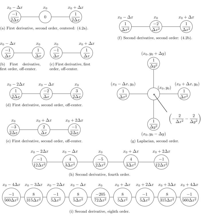
4.1 Graphical representation of finite differences for approximating various derivatives at a point x = x0. The circles correspond to grid points and the numbers inside are the coefficients
by which the function being differenced should be multiplied at each grid point before being summed. This should give some indication why the terms “stencil” and “molecule” are often used. It should also give some indication of the variety of possible stencils in terms of size, accuracy order, derivative, centered vs off-centered, and in different dimensions. . . 39
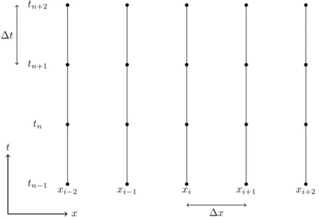
4.2 A representation of the method of lines in thetx-plane. . . 42
5.2 Surfaces of constantt0 andx0 in various coordinate systems. The zig-zag line shows the black hole’s worldline. Fig. 5.2g shows why the height function cannot be applied immediately after the Lorentz boost (shown in Fig. 5.2b); the spatial slices intersect, as the divergence is centered at the location of the black hole. In contrast, if we apply a Galilean boost in the opposite direction (shown in Fig. 5.2c) the location of the puncture does not move so that the slices do not intersect when applying the height function (shown in Fig. 5.2d). Note the singularity is no longer covered by the coordinates after the radial rescaling is done (shown in Fig. 5.2e). . . 54
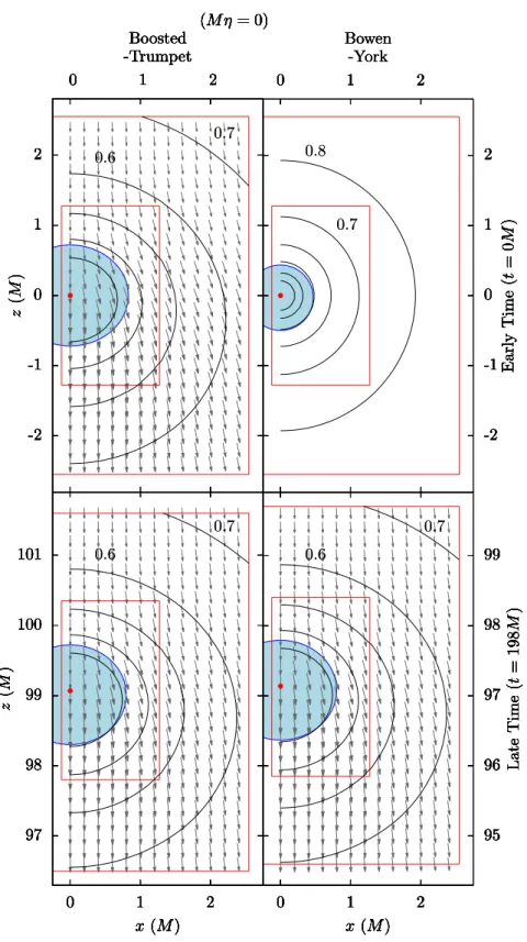
5.3 Equatorial slices showing lapse, shift, puncture location, apparent horizon, and AMR bound-aries. Top images show the initial time slice and bottom images are at late time (t= 198M). Left images are for boosted-trumpet data and right images are for Bowen-York data. On the initial time slice for Bowen-York βi = 0. In all cases, two of the lapse contours are labeled, other contours are evenly spaced in lapse value. All four slices have equal scales except that the two late time images are at different locations (because the Bowen-York black hole had a lower average speed than the boosted-trumpet black hole, see Fig. 5.7). In both cases, the black holes havev= 1/2 in the positivez direction. . . 63
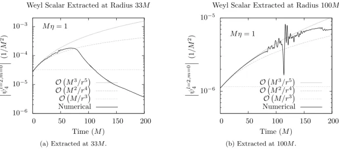
5.4 Comparison of analytic and numerical computations of gravitational waves. The left (right) subfigure show thel= 2,m= 0 mode ofψ4 evaluated at a coordinate radius of 33M (100M).
The black line is a numerical result from a simulation. The gray lines show approximations given by (5.53) to various orders. We can see the approximation (5.53) breaking down near t≈66M (t≈200M), as discussed in in the text. . . 66
5.5 Resolution dependence of thel = 2, m= 0 mode of ψ4 extracted from three simulations at
coordinate radiusr= 100M. . . 67
5.6 Dominant mode of the Weyl scalarψ4 extracted at coordinate radii 33M and 100M. Note
that the Weyl scalar computed in the Bowen-York simulations does indeed have the same background growth. This simulation usesM η= 1. . . 68
5.7 Speed of black holes computed from shift norm as a function of simulation time. These black holes have v = 0.5. Dashed lines correspond to simulations with M η = 1 and solid lines to simulations with M η = 0. Black lines are boosted-trumpet black holes, blue lines are boosted-trumpet black holes except with zero initial shift, and the red line is a Bowen-York black hole. . . 68
5.8 Speed of black holes with v = 0.85 as measured by shift and Lorentz factor (5.54) from v = p1−1/γ2. These values are not accurate at late time because of the difficulty in
extrapolating the ADM momentum when the black holes get closer to the extraction surfaces. 69
5.9 The speed of a boosted-trumpet black hole for a number of specified speeds. . . 70
5.11 Ratios of circumferences of the apparent horizon as functions of simulation time. These black holes have speeds set to v = 0.5. See (5.49) for how the circumferences are computed. We only show one of the two polar circumferences we could have computed here (i.e., we show Cxz but notCyz); the analogous plot comparingCyz andCxyis indistinguishable by eye from
this one. Note that the boosted-trumpet data has less distortion than the Bowen-York data both at early times and late times. . . 71
5.12 Relative error of simulated values ofMADMandPzADM. . . 72
5.13 ADM mass-energy as a function of ADM momentum up to vmax = 0.95. The blue curve
shows the analytic values expected from (5.41) and (5.42), black dots show the numerical values extrapolated to infinity, and red diamonds and gray squares show the numerical values calculated at 100M and 33M, respectively. The values computed at 33M are much less accurate than the extrapolated values, but the values computed at 100M (which are mostly hidden by the extrapolated data points) are also less accurate than the extrapolated values. . 73
5.14 The average value of the mean curvature of the spatial slice at the location of the apparent horizon as a function of simulation time. This simulation starts with advection in the lapse gauge condition on, it is turned off att = 22.5M and back on again at t= 72.5M. This is intended as a consistency check with [30] (see their Fig. 21). It also hasM η= 2 and advection turned off in the Γ-driver gauge condition. The insets show relative error as a function of time calculated as|K(0)−K(t)|/K(0). . . 74
5.15 Coordinate radius of the apparent horizon as a function of simulation time. The simulations start with advection in the lapse gauge condition on, it is turned off att= 22.5M, and back on again at t= 72.5M. This is intended as a consistency check with [30] (see their Fig. 22). Both simulations have advection turned off in the Γ-driver gauge condition. The solid line corresponds toM η= 0 and the short dashed line corresponds toM η= 2. . . 74
5.16 Violation of the Hamiltonian constraintHalong thez-axis on the initial time step for boosted-trumpet (black) and Bowen-York (red) initial data. These black holes have v = 0.5 in the positivez direction. . . 75
5.17 Top: Resolution dependence of the Hamiltonian constraintH and momentum constraintMz
along thez-axis on the initial time step for boosted-trumpet initial data. The black curve has grid spacing ∆x= 0.8M on the coarsest level, the red and blue curves have grid spacings of
2
3∆xand 4
9∆x, respectively. These black holes havev= 0.5 in the positivezdirection. In the
inset, the AMR boundaries are shown on the left side by gray lines; AMR boundaries on the right side are not marked, but are at the same distances and should be visible as discontinuities in the curves. Bottom: Same except that the constraint violations from the medium and high resolution simulations have been multiplied by (3/2)4 and (9/4)4, respectively. . . 76
6.1 Flowchart showing how superposed initial data is computed. The spacetime quantities are decomposed into the ADM quantities and then the conformal quantities. Then these conformal quantities are superposed according to (6.1) and finally the physical ADM quantities are reconstructed. . . 78
6.3 Violation of the Hamiltonian constraint with two black holes superposed along the z-axis, comparing Bowen-York initial data to boosted-trumpet initial data. Even without re-solving the constraint equations, the boosted-trumpet initial data violates the Hamiltonian constraint only by a couple orders of magnitude more than the Bowen-York data. The violation of the momentum constraint is comparatively much larger because Bowen-York data satisfies the momentum constraint by construction; the violation is therefore only due to the finite differencing used to compute the derivatives in the constraint equation (the AMR boundaries are visible where the resolution changes). . . 79 6.4 The growth in the asymmetry of the puncture trajectories for both boosted-trumpet and
Bowen-York black hole binaries. Since it should be symmetric about the y-axis, the sum of the puncture locations should be zero~x1+~x2 = 0. Given that this is a semi-log plot, it
appears that the asymmetry in both binaries is growing approximately exponentially (though, the asymmetry in boosted-trumpet binary may be super-exponential). . . 81 6.5 The real part of the l= 2, m = 2 mode ofψ4 extracted at a radius of 100M for the binary
boosted-trumpet and Bowen-York black holes. Grey lines correspond to the times shown in Fig. 6.6 and Fig. 6.7. The Bowen-York data ends due to CPU-hour constraints, not because of physical or numerical limitations. . . 82 6.6 Equatorial slices showing evenly spaced level sets of the lapse (with labels), shift vectors,
puncture locations, puncture trajectories (between snapshots), apparent horizons, and AMR boundaries at four times throughout evolution. The asymmetry in the trajectories is apparent in the last frame. . . 83 6.7 Same as Fig. 6.6 except with Bowen-York initial data. . . 84 6.8 The trajectories of the punctures in the binary simulation. Initial data was symmetric under
a rotation ofπ about they-axis. The trajectories do not retain this symmetry though. This is particularly evident in the inset, where one trajectory has been rotated so that the two trajectories initially line up. . . 85 6.9 Same as Fig. 6.8 except with Bowen-York initial data. In the inset, theπ-rotated trajectory
is visually coincident with the other trajectory (though, see Fig. 6.4 for evidence that there is a growing asymmetry even in the Bowen-York black hole trajectories). . . 86
7.1 Figure showing relevant vectors for rotation of initial data via a spatial coordinate transfor-mation (in theφv = 0 plane for visual simplicity). . . 89
7.2 Penrose diagrams for the Kerr spacetime with two trumpet slicings. The zigzag line shows r= 0 (which is not singular off of the equatorial plane) and the inner and outer horizons at r = r± are shown with dashed lines. On the left the limiting radius of the trumpet slices r−< r < r+ is shown by the dotted line and on the right the limiting radius of the trumpet
LIST OF ABBREVIATIONS AND SYMBOLS
ADM Arnowitt, Deser, and Misner
LIGO Laser Interferometer Gravitational-Wave Observatory
AMR adaptive mesh refinement
BSSN Baumgarte, Shapiro, Shibata, and Nakamura
LHS, RHS left hand side and right hand side of an equation
CFL Courant-Friedrichs-Lewy
ODE ordinary differential equation
M spacetime manifold
gab,g spacetime metric onMwith signature (−,+,+,+) and its deter-minant
a,b, c,d,e,f, . . . spacetime indices, running from 0 to 3 (t, x, y, z ort, r, θ, φ)
Γ
(4) a
bc,∇a Christoffel symbols and covariant derivative compatible withgab
R
(4)
abcd, C (4)
abcd, R (4)
ab, R (4) ,G
ab Riemann tensor, Weyl tensor, Ricci tensor, Ricci scalar, and
Ein-stein tensor describing the curvature ofM
Σ spatial slice in the foliation of M
na,ta,ω
a, Ωa normal vectors to Σ and related 1-forms
Pab operator to project object “into” spatial slice: P
a b =δ
a b +n
an b
γij,γ spatial metric on Σ with signature (+,+,+) and its determinant
i,j,k,l,m,n, . . . spatial indices, running from 1 to 3 (x, y, zorr, θ, φ)
Γi
jk, Di Christoffel symbols and covariant derivative compatible with the
spatial three-metricγij
Rijkl, Rij,R three-dimensional Riemann tensor, Ricci tensor, and Ricci scalar describing the intrinsic curvature of Σ
α,βi,K
ij, K lapse, shift, extrinsic curvature, and mean curvature describing
S 2-sphere slice in the foliation of Σ
qAB, q angular metric onS and its determinant
A,B angular indices, running from 2 to 3 (θ andφ)
σ,ωA lapse and shift analogs describing foliation of the spherical surfaces
within a spatial slice
dΩ area element of a spheredΩ≡sinθdθdφ
H,Mi Hamiltonian constraint violation (2.48a) and momentum constraint
violation (2.48b)
δa
b, εabcd,εijk Kronecker delta and totally anti-symmetric tensors
L Lie derivative
Tab,Sij,Si,S,ρ stress-energy tensor and its projections (2.30)
R the Schwarzschild radial coordinate
f 1−2M/R
TT the transverse-traceless piece of a tensor
˜ a conformally related quantity
˜
γij,ψ, φ,Wi,A
ij, ˜Aij, ˜A ij T T, ˜A
ij
L pieces of the conformal decomposition
˜ LW
ij
,∆˜LW
i
symmetrized transverse-traceless gradient (2.65) and vector Lapla-cian (2.68)
˜
Rij,Rijφ, ˜Γi, ∂0 quantities for the BSSN equations (2.75)
hab, (1)hab, (2)hab perturbations to the spacetime metricgab
ka, la,ma,ma null tetrad basis vectors
MADM,PADMi ,J i
ADM ADM mass, momentum, and angular momentum
Θ expansion of outgoing light rays at the horizon
MS,JS,RS,AS mass and angular momentum defined by symmetries on the horizon and radius and area of the horizon
ψ0, ψ1,ψ2,ψ3,ψ4 Weyl scalars
I,J Weyl curvature invariants
e×ab, e+ab,h×,h+ tensor wave polarizations and their amplitudes
ð,ð derivative operators for raising and lower spin weights
Y
s lm spherical harmonic of spin weights
TabGW stress-energy of GWs
LGW luminosity of GWs
R
(1)
ab, R (2)
ab perturbations to the Ricci tensor
h i time average over many GW cycles
F Fourier transform
L,U,D, . . . matrices
~
CHAPTER 1: Introduction
Historically, tests of general relativity have taken place in our solar system and were generally only able to probe the weak field limit. This has changed with the recent rapid progress in the field of gravitational wave astronomy. In the past two years, this new field has given us novel tests of general relativity, not possible within our own solar system. As instrument sensitivities are increased, it promises to provide more stringent tests in the future. In order to properly understand observations, comparisons with theory must be made. Accurate methods exist for simulating highly relativistic systems, but there is the non-trivial issue of how to initialize simulations. This project provides improved methods for computing initial data. This Chapter gives an overview of tests of general relativity, simulation methods, and what this project has accomplished.
Section 1.1: Testing General Relativity Through Gravitational Wave Astronomy
One of the most famous tests of general relativity which has been carried out in the solar system is the perihelion advance of Mercury: the measured value (42.98±0.04)00/century [43] is in remarkably good agreement with the value calculated from theory 42.9800/century [43]. The Cassini-Huygens spacecraft was able to perform measurements of the Shapiro time delay during its flight to Saturn and measured the parameterized post-Newtonian parameter γ; if general relativity is correct it is expected thatγ = 1. The measured value γ−1 = (2.1±2.3)×10−5 [55] is consistent with zero, indicating that no deviation from
general relativity was detected. Violations of the weak equivalence principle have been constrained to be at most a few parts in 1013by E¨otv¨os-type experiments [54]. These are only a few of many tests. None of these
findings have contradicted general relativity, but they have only tested it in the weak field limit.
Observations of the Hulse-Taylor pulsar have probed general relativity in an environment with a stronger gravitational field. This pulsar is one of two neutron stars forming a binary system [31]. The observed time rate of change of the orbital period of this binary system (−2.396±0.005)×10−12 is once again
remarkably close to the predicted value (−2.402531±0.000014)×10−12 [55].1 This is generally seen as the
first observational evidence for the existence of gravitational waves, but the measurement was made through electromagnetic observations and is therefore somewhat indirect.
1Using 31 557 600 s = 1 year, these values correspond to (75.6±0.2) µs/year (observed) and (75.8181±0.0004) µs/year
It is only with the recent detections by the advanced Laser Interferometer Gravitational-Wave Obser-vatory (LIGO) that we have obtained our first direct measurements of gravitational waves. The first four detected events – dubbed GW150914 [6], GW151226 [11], GW170104 [12], and GW170814 [8] – were each generated by the co-orbital motion and merger of a pair of black holes. The fifth detection – GW170817 [9] – was of a signal from the merger of two neutron stars. But the existence of gravitational waves is not the only strong field test of general relativity that gravitational wave astronomy can provide. The mass of the graviton was constrained to be less than 1.2×10⁻²² eV (corresponding to a Compton wavelength
of over a lightyear) [7] by the dispersion of gravitational waves detected from GW150914. Additionally, GW150914 allowed for constraints on deviations from general relativity, even if some of these constraints are not particularly strong [7].
To be able to connect the raw data of the detection to a physical model of the emitting system we must have a well developed understanding of general relativity [10]. General relativity is non-linear, which makes it difficult to work with mathematically. Perturbative methods exist to handle its non-linearities iteratively, including black hole perturbation theory and post-Newtonian expansions [35, 42, 22]. These methods require restrictive physical properties, such as a small ratio between the masses of the orbiting objects or low velocities; the signals detected by LIGO came from systems which do not possess these properties. Therefore, for these systems, perturbative processes break down and Einstein’s equations must be solved ‘all at once.’ To distinguish it from perturbative methods, this ‘all at once’ method is called numerical relativity [20, 13]. Although all of these methods inform one another, are important, and ultimately must all be understood to get the fullest picture of general relativity, numerical relativity is currently our only tool to model the inspiral, merger, and remnant of compact binaries that are being observed.
Section 1.2: Numerical Relativity
One downside of numerical relativity as compared with other methods is the relative difficultly in con-structing initial data for a simulation. Consider briefly a simulation of electromagnetic fields. Two of Maxwell’s equations (Coulomb’s law and∇ ·~ B~ = 0) constrain the possible configurations of the electric and magnetic fields, and these constraints must be satisfied at any time. When starting a simulation, data must be given for the electric and magnetic fields which satisfies these constraints. This may require solving a Poisson equation for the initial electric potential, for example. Similarly, Einstein’s equations do not allow for arbitrary configurations of the gravitational field, and it is non-trivial to pose initial data which is properly constrained.
state-of-the-art initial data in use with the Einstein Toolkit is based on the Bowen-York formalism [23, 57]. This formalism makes mathematical assumptions in order to greatly simplify the constraint equations, allowing valid initial data to be computed more easily. This data solves the constraint equations, which is required for a mathematically valid solution to Einstein’s equations. It does not, however, accurately model the intended physical system. As we will see, initial data computed this way contains non-physical ‘junk radiation’ which initially distorts the space near the black holes and is released as gravitational waves at the start of the simulation. This junk signal robs the black holes of energy, momentum, and angular momentum and contaminates the physically relevant gravitational wave signal.
In order to distinguish the junk signal from the physical gravitational wave signal which appears later, the black holes must be started farther apart (increasing the duration of the simulation) and the boundary of the simulation domain must be farther out (to reduce the impact of reflected waves on the simulation). Both allowances drive up the computational cost of a simulation, but this is not the only problem with junk radiation. Areas of parameter space are precluded as the energy and angular momentum carried away by junk radiation limits the range of spins and momenta of black holes that can be simulated. Because astrophysical black holes are expected to have large spins, this limitation on spins is more than just a pedantic concern [33].
Clearly, it would be advantageous to have an alternate method for constructing initial data. However, the method by which the black hole singularity is handled numerically plays a large role in how initial data can be constructed. One method for handling singularities is the so-called ‘excision’ method. In this method, the interior of the black holes – where large gradients and infinite values are present – are removed from the simulation domain. This creates the need to specify interior boundary conditions and remove a roughly ellipsoidal region from a cubical lattice; but information cannot leave a black hole in classical general relativity so there is no need to simulate its interior. This method has been found to be amenable to using a Lorentz-like coordinate transformation to boost a black hole written in Kerr-Schild coordinates to generate initial data [34], as well as initial data modifications to reduce junk radiation content [49, 50].
The Einstein Toolkit does not use excision, instead it uses the ‘moving punctures’ method. Moving punctures is the name given to a specific set of choices for the spacetime coordinates.2 Like excision, a
moving punctures coordinate system has the effect of removing a black hole’s singularity from the simulation domain. However, unlike excision, moving punctures does not remove any points from the simulation grid. Instead, the coordinates are engineered so that they only cover a portion of the spacetime manifold away from the black hole singularities; this coordinate patch corresponds to the simulation domain. This can be
accomplished using a so called ‘trumpet slicing,’ a specific topology where the spatial slices reach a limit a finite distance away from any singularities. The moving punctures gauge is not the only coordinate system that gives trumpet slicing, but it is an example of trumpet slicing which is well suited to numerical work.
It has been shown that, over the course of a simulation, the moving punctures gauge conditions drive Bowen-York initial data away from its initial (non-trumpet) slicing to trumpet slicing [30]. Trumpet slicing has been explored for non-moving, non-rotating [25] and non-moving, rotating black holes [26] in a gauge other than moving punctures, and also for a non-moving, non-rotating black hole in the moving punctures gauge [30]. Recent attempts to decrease junk radiation content of initial data within the moving punctures scheme have focused on relaxing one of the Bowen-York assumptions without using trumpet slicing [46].
Section 1.3: Project Goals
We have discussed the importance of strong field tests of general relativity, the importance of numerical relativity to these tests, and the importance of well constructed initial data to numerical relativity. The goal of this project has been to improve the Einstein Toolkit by improving the tools available for construction of initial data, utilizing the specific trumpet slicing that is the steady state of the moving punctures gauge.
At its core, this work has combined the ideas of trumpets in moving punctures gauge and a Lorentz boosted Schwarzschild black hole. By creating a series of coordinate changes, we transform a black hole written in a common coordinate system to a black hole with both non-zero coordinate velocity and trumpet slicing adapted to the moving punctures gauge.
To understand the big picture better, return momentarily to the electromagnetic simulation considered above. Suppose we have initial data for the vector potential which we know gives electric and magnetic fields which satisfy Maxwell’s two constraint equations, but that this initial data is not well suited to our numerical methods. We might then apply a gauge transformation to this vector potential to obtain different initial data which models the same physical situation (i.e., the electric and magnetic fields are unchanged). The result is guaranteed to satisfy the constraint equations, and this known without explicitly solving them. This is analogous to what we propose here: we start with Schwarzschild spacetime in the familiar Schwarzschild coordinates (a simple, known solution to the constraints that is not well suited for simulation) and apply a series of coordinate (gauge) transformations to get it in a form that may look more complex, but represents the same physical situation.
apparent. A large part of this project has been concerned with the interpretation of the properties of the resulting coordinate system.
Section 1.4: Outline of the Remainder of the Thesis
Chapters 2 through 4 give overviews of various required aspects of simulating black holes. With that foundation laid, we then discuss novel methods for constructing initial data and the results of this project, found in Chapters 5 and 6. Throughout this work, we use units where G= 1 =c,3 the spacetime metric
signature is (−,+,+,+), and sign conventions are those of Misner, Thorne, and Wheeler [35].
Chapter 2 discusses a number of formalisms needed to carry out numerical relativity simulations. There we make explicit the formulation of Einstein’s equations as a Cauchy initial value problem and explore the options for solving for initial data, including the Bowen-York method.
Chapter 3 gives an overview of how a number of physical properties of spacetimes are extracted from simulations. Among these properties are the energy, momentum, and angular momentum contained in a spacetime, the gravitational wave content of the spacetime, and black hole horizon properties.
Chapter 4 gives a very brief overview of relevant numerical methods and how the Einstein Toolkit im-plements them.
Chapter 5 describes our new method for constructing initial data. We compare results from this data to those found using Bowen-York data. We find that it is well adapted to the moving punctures gauge conditions and contains orders of magnitude less junk gravitational waves than the Bowen-York data. We also carry out analysis to gain a thorough understanding of the properties of the new coordinate system we have created.
Chapter 6 examines preliminary results of a binary composed of boosted-trumpet black holes. The initial data for this binary system is constructed by a simple superposition of the data for a single black hole.
Finally, Chapter 7 summarizes our findings.
CHAPTER 2: Decomposing Spacetimes and Einstein’s Equations
In order to be dealt with numerically, Einstein’s equations must be separated into space and time parts. This breaks their inherently covariant nature but does allow for a formulation in terms of a Cauchy problem, which is more amenable to numerical evolution. We describe a formalism for decomposing spacetime and Einstein’s equations in this Chapter.
In the first section of this Chapter, we will foliate the spacetime manifold M by dividing it into a collection of three-dimensional spacelike surfaces Σ. Each Σ can be interpreted as representing the universe at an instant in time, and collectively the Σ cover the portion ofMin which we are interested. We will then compute curvature quantities for the spatial slices and relate them to the curvature quantities describing M. These quantities will allow us to decompose Einstein’s equations via temporal and spatial projections. Finally, we will specialize to a specific basis to bring out a time derivative, culminating in the Arnowitt, Deser, and Misner (ADM) equations [20, 28, 56]. In investigating the nature of the ADM equations, we will see the consequences of general relativity’s coordinate freedom and how it can be used to improve numerical stability.
The second section carries the decomposition one step further, foliating a spatial slice into a collection of surfaces which are topologically spherical. This allows us to define the idea of trumpet slicing. The final section outlines a conformal decomposition which is useful in numerically solving the constraint equations obtained in section 2.1 in order to give initial data in practice.
Section 2.1: ADM Formalism for Foliation and 3+1 Decomposition of Spacetime
Before investigating the exact nature of the decomposition, we look to see generally how it must come about. Consider the twice contracted Bianchi identity
∇bGab= 0, (2.1)
and Einstein’s equations with indices raised
Separating the Bianchi identity into the timelike derivative and spatial derivatives, we find
∇0G a0=
−∇iG
ai. (2.3)
Because Gab is a curvature quantity which is constructed from derivatives of the metric, including second
derivatives,∇iGaicontains at most second time derivatives ofg
ab. Therefore,∇0Ga0contains at most second
time derivatives and soGa0 contains at most first time derivatives. Thus, four of Einstein’s equations,
Ga0= 8πTa0, (2.4)
relate the metric and its first time derivatives, and are therefore constraint equations which must be satisfied initially and at all subsequent times. The evolution equations are the remaining six Einstein’s equations,
Gij= 8πTij, (2.5)
which govern the evolution of the spacetime. The system may appear under specified as there are only six evolution equations for the ten metric components. However, there are four degrees of gauge freedom corresponding to coordinate changes; specifying four equations in order to fix the coordinate system brings the total number of equations back up to ten. Given these considerations, it is perhaps not surprising that we will find that doing at least one temporal projection gives us a constraint while two spatial projections will give us evolution equations.
Analytically, if the constraint equations are satisfied initially, they will continue to be satisfied. We see this because
∇b G ab
−8πTab
= 0 (2.6)
which means
∇0 Ga0−8πTa0
=−∇i Gai−8πTai
. (2.7)
If, on some slice, data is given which satisfies Einstein’s equations, the RHS of (2.7) will be zero. The LHS then tells us that the value of the constraint violation will not change away from the initial slice. This means that if the constraints are satisfied at one time then, analytically, they must be satisfied at all times. Compare this with Maxwell’s equations, where∇ ×~ E~ =−∂ ~B/∂trequires that∇ ·~ B~ = 0 remain true if it is satisfied initially.
a normal vector to the surfaces by working with the gradient of ˜t. To this end, define a one-form as the exterior derivative of ˜t
ωa ≡ d˜t
a. (2.8)
Note that, in general,ωa is timelike and will have a variable norm
gabωaωb =−α−2. (2.9)
This defines the ‘lapse’ functionα. With this we can create another timelike one form which is unit normalized
Ωa ≡αωa (2.10)
so that
gabΩaΩb=−1. (2.11)
The unit normal vector is then
na≡ −gabΩ
b, (2.12)
it is also timelike
nana =−1, (2.13)
where the sign in (2.12) is chosen so thatna points in the future direction (increasing ˜t) when the lapse is positive
na∇a˜t=n aω
a =α−
1. (2.14)
There are many timelike vector fieldstawhich satisfy the normalizationωata= 1 relative to the foliation.
One possible choice fortaisαna, but we are free to add a vectorβa (called the ‘shift’ vector) which satisfies naβa = 0 but is otherwise arbitrary, and still maintain the normalization
ωa(αna+βa) = 1. (2.15)
Spatial coordinates are dragged from time slice to time slice in the directionta. In this way, the decomposition
ta=αna+βa (2.16)
We will find these two quantities very important moving forward, where their interpretation will be more fully explored. Equations governing the evolution of α and βa will determine the coordinate system and,
as mentioned above, complement the six evolution equations coming from Einstein’s equations to give ten equations needed to specify the dynamics of the ten independent pieces of the spacetime metricgab.
Contracting a vector with −nan
b gives its projection in a timelike direction, so−n an
b can be thought
of as a temporal projection operator. If Va is a vector such that Vana = 0 then V0 is not algebraically independent from Vi and the vector Va has three degrees of freedom, effectively containing no timelike information. The same idea holds for tensors of all ranks and index structures. In general, a tensor is said to be ‘spatial’ when all of its contractions withna (orn
a) give zero. When dealing with spatial tensors, we
are free to disregard any timelike components; as we have seen, they are not independent and – if needed – we can recover them by contracting withna, setting the result equal to zero, and solving algebraically. We
will make liberal use of this in the future and for simplicity’s sake often only consider the spatial indices. A spatial projection operator can also be constructed fromna
Pab ≡δ a b +n
an
b. (2.17)
Consider an arbitrary (in particular, not necessarily spatial) covectorCa acted on byPab andn b
nbPabCa =nb(δba+nanb)Ca = (na−na)Ca = 0. (2.18)
As can be seen, this result is independent ofCa and thus demonstrates howPa
bCa is spatial by virtue of the
construction ofPa
b. When every index of a tensor has been projected into Σ byPab, the tensor is guaranteed
to be spatial.
By projecting the spacetime metricgab into Σ, we obtain a ‘spatial metric’
γab ≡Pc aP
d
bgcd=gab+nanb (2.19)
which makes Σ a Riemannian manifold in its own right. The spatial metric is positive definite and can be used to raise and lower indices of spatial tensors. The covariant derivativeDa in Σ arises naturally from the geometric structure ofM: first the spacetime covariant derivative∇a is taken and then every index of the result is projected into Σ. With this definition,Da can be shown to be compatible withγab
Daγbc≡PdaPbePfc∇dγef =PdaPebPfc ne∇dnf+nf∇dne
Thus, we know it must also be possible to find connection coefficients forDa
Γijk≡ 1 2γ
il γ
lk,j+γjl,k−γjk,l
, (2.21)
and covariant derivatives in Σ can be computed without reference to the geometric structure ofM. All the other usual intrinsic curvature quantities can be similarly defined in Σ; in particular, the curvature of Σ is described by a three-dimensional Riemann tensorRi
jkl, a Ricci tensorRij, and a Ricci scalar R (when
we need to refer to curvature quantities of the four-dimensional spacetime we will indicate them with a (4); e.g., (4)Rabcd). The three dimensional tensors in Σ transform as expected under changes of the spatial coordinates, but not under coordinate changes involving time. Expressions involving spatial tensors are therefore covariant in a restricted sense. These last two points serve to reemphasize that Σ is a Riemannian manifold with a geometric structure independent from that ofM.
So far, all curvature quantities have been defined completely in terms of the intrinsic geometry of Σ. In order to make connections between Ri
jkl and R (4) a
bcd, we will need a notion of how Σ curves in and is
embedded withinM. We make this connection by examining how the spatial metric changes as you move from Σ to a neighboring spatial slice in the foliation. Specifically, this is accomplished by Lie draggingγab along the normal vectorna. The extrinsic curvature is defined by
Kab ≡ −
1
2Lˆnγab =− 1 2(n
c∇
cγab+γcb∇anc+γac∇bnc). (2.22)
Because na is timelike, this definition captures the (rough) idea that the extrinsic curvature measures the
time rate of change of the spatial metric. It can be shown from this definition that
Kij =−Pa iP
b
j∇(anb), (2.23)
from which it is apparent thatKij is symmetric and spatial.
The symmetries(4)Rabcd=−(4)Rbacdand(4)Rabcd=−(4)Rabdcmean that projecting the Riemann tensor three or more times ontonb gives zero identically (e.g.,nanbnc(4)Rabcd=−nanbnc(4)R
bacd necessitates that
nanbnc(4)Rabcd= 0). Thus, we consider four spatial projections of(4)Rabcd (Gauss’s equation), three spatial and one temporal projection of(4)Rabcd (Codazzi’s equation), and two spatial and two temporal projections of (4)Rabcd (Ricci’s equation). After some calculation (the details of which are omitted), we find
PaiP b jP
c kP
d
l R
(4)
PbiP a jP
c kn
d
R
(4)
abcd=DiKjk−DjKik (Codazzi) (2.25)
PdiP b jn
cna(4)R
abcd=LnˆKij +α
−1D
iDjα+KkiK k
j (Ricci). (2.26)
Contracting Gauss’s equation twice and Codazzi’s equation once gives
γacPdiP b
j R
(4)
abcd=Rij+KKij−K k
i Kjk (2.27)
γacγbd(4)Rabcd=R+K2−KijKij (2.28) Pbin
dγac(4)R
abcd=DiK−DjK j
i , (2.29)
where the mean curvature is defined asK= Tr(K) =Ki i .
Define projections of the stress-energy tensor
ρ≡nanbTab, Si ≡ −PainbTab, Sij ≡PaiPbjTab, and S ≡γijSij. (2.30)
Also compute projections of the Einstein tensor
2nanbGab=γacγbd(4)Rabcd and PianbGab=γacPbind(4)Rabcd. (2.31)
Einstein’s equations and Gauss’s equation contracted twice (2.28) give the Hamiltonian (or energy) constraint
16πρ= 16πnanbTab = 2nanbGab=γacγbd(4)Rabcd =R+K2−KijKij. (2.32)
Einstein’s equations and Codazzi’s equation contracted once (2.29) give the momentum constraint
8πSi =−8πPain bT
ab =−P a in
bG
ab=−γ ac
Pbin d(4)R
abcd=DjK j
i −DiK. (2.33)
The constraints do not involve time derivatives, instead they relate the variablesγij,Kij, and their spatial derivatives at all times (again, recall the case of Maxwell’s equations where ∇ ·~ B~ = 0). Noting that both these equations derive from one or more temporal projections of Einstein’s tensor it makes sense that they are constraint equations, given the discussion of the Bianchi identity at the beginning of the section.
calculateLˆtγij andLtˆKij. The first evolution equation is
Ltˆγij =αLˆnγij+Lβˆγij =−2αKij +Diβj+Djβi. (2.34)
The second involves Ricci’s equation
LtˆKij =αPdiP b jn
anc(4)R
abcd−α
−1D
iDjα−KkiK k j
+LβˆKij. (2.35)
But Gauss’s equation (2.27) and the trace-reverse of Einstein’s equations give
PdiPbjnanc R (4)
abcd=γ ac
PdiPbj R (4)
abcd−P a iPbj R
(4) ab
=Rij+KKij −KikKjk−PaiP b
j(8πTab −4πT gab)
=Rij+KKij −KikKjk−8πSij+ 4πγij(S−ρ), (2.36)
so that
LtˆKij =α Rij+KKij −2KikKjk −8πSij + 4πγij(S−ρ)
−DiDjα
+βkDkKij +KikDjβk+KkjDiβk. (2.37)
This second evolution equation came from two spatial projections of Einstein’s equations, again reflecting the discussion at the beginning of the section on the Bianchi identity. Notice that the six second-order evolution equations have now been recast as twelve first-order evolution equations. The first evolution equation essentially came from the definition of the extrinsic curvature in terms of the Lie derivative of the spatial metric, which we saw before makes the extrinsic curvature something like a time derivative of the spatial metric. This reduction of order in the evolution equations is therefore analogous to reduction of order in the simple system
d2
dt2x(t) =a(t) ⇒
d
dtx(t) =v(t)
d
dtv(t) =a(t)
(2.38)
withγij playing the part of the coordinatex(t) andKij the part of the velocityv(t).
basis vectors lie in a spatial slice. Therefore, these three basis vectors (ei) a
satisfy
ωa(ei) a
= 0. (2.39)
We will also want this basis to be unchanged between slices
Ltˆ(ei)a = 0. (2.40)
If both of these desired properties are to hold, we must have
0 =Lˆt(ωa(ei) a
) = (ei) a
Ltˆωa+ωaLtˆ(ei) a
= (ei) a
Ltˆωa (2.41)
which can only be true in general ifLˆtωa = 0, but we see that this is the case
Ltˆω=Ltˆdt˜=d Lˆtt˜
=d ta∇a˜t
=d(taωa) =d (αna+βa) −α−1n a
=d(1 + 0) = 0. (2.42)
To complete our basis, we take (e0)a =ta. With the definitions of the other three basis vectors, we know
ta = (1,0,0,0) in this basis. Note that
LtˆTab =t cT
ab,c +Tact c
,b+Tcbt c
,a=∂tTab. (2.43)
It can be shown that the same holds for more general tensors, so Lˆt the Lie derivative along ta is just a partial derivative with respect to timet in this basis.
In this basis, the following matrix representations for a number of quantities can be found
ta=
1 0 0 0
na=α−1
1 −βi
β
a =
0 βi
na= (−α,0,0,0) γab=
0 0
0 γij
γab=
βiβi βi βj γij
, (2.44)
representations forgab andgab
gab=
βiβi βi βj γij
−
α2 0
0 0
=
βiβi−α2 βi βj γij
(2.45)
and
gab=
0 0
0 γij −α
−2
1 −βi
−βj βiβj
=
−α−2 α−2βi
α−2βj γij−α−2βiβj
. (2.46)
The line element is
ds2= −α2+βiβ i
dt2+ 2βidxidt+γijdxidxj
=−α2dt2+γ ij dx
i+βidt
dxj+βjdt
. (2.47)
These forms of the line element illustrate again the interpretation ofαandβi as determining the coordinate
system (or more specifically, the evolution of the coordinate system in moving from Σ to a nearby spatial slice). It is helpful to think of the lapse as specifying the rate at which time is passing between slices and the shift as describing how the spatial coordinates move from one slice to the next. Between two slices separated by a coordinate timedt, the proper time of an observer moving along the normalna increases by
an amountαdt and the spatial coordinates shift by an amountβidt. This is shown in Fig. 2.1. Also note
thatα2=−g/γ.
A few words are in order about the final form of the ADM equations we use. We will now specialize to the case of vacuum where Tab = 0 (with the exception of parts of §3.1 and §3.2). We also defineH and Mi as shorthands for the Hamiltonian and momentum constraint equations, respectively. These quantities are analytically zero, but are useful to refer to none the less, especially as diagnostics of numerical results. Reproduced together for easy reference, we have our final form for the ADM equations
0 =H≡R+K2−KijKij (2.48a)
0 =Mi ≡DjKij−DiK (2.48b)
∂tγij =−2αKij +Diβj+Djβi (2.48c)
∂tKij =α Rij+KKij −2KikKjk−DiDjα+βkDkKij +KikDjβk+KkjDiβk. (2.48d)
Σ(t1) Σ(t2)
xa 0(t1)
α∆tna
xa0(t2)
∆tβa
γij(t1), Kij(t1)
γij(t2), Kij(t2)
Figure 2.1: The foliation of spacetime. Shown are two moments in time, Σ(t1) and Σ(t2), in the foliation,
each with its ownγij andKij. The relationship between a point xa0 in the two members of the foliation in
terms of αandβi also is shown. Analytically, there are an infinite number of such slices; numerically, the
code computes quantities at the two timest1andt2separated by some small ∆t.
their formalism [17]). A more geometric approach was taken here (and in e.g., [20, 13, 57]) because it gives helpful insight into how data is evolved from one spatial slice to the next during a simulation. However, the original approach does highlight two important features, reinforcing results obtained here. The first feature is that the extrinsic curvature is related toπij, the generalized momenta conjugate toγij. Thus, the reduction in order we saw earlier comes naturally from a Hamiltonian mechanics approach. Secondly,αand βi arise as Lagrange multipliers, multiplyingH andM
i, respectively. This further emphasizes that they are
freely specifiable.
2.1.1: Gauge Choice
Now, contract the evolution equation for the spatial metric (2.48c) using Jacobi’s formula
∂tlnγ=−2αK+ 2Diβi. (2.49)
Assume for now that we have chosen a gauge where βi= 0. Near the black hole, where α≈0 (i.e., proper
time passes more slowly near the singularity), this tells us that
This is a desirable property because – if γ does not change near the black hole – then volumes will be preserved and a coordinate singularity is avoided. If the volume were to become too small, freely falling observers would “crash” into each other. Therefore, we can demand the lapse satisfy the equation
∂tα=−2αK (2.51)
to drive the term 2αK toward zero and achieve this. Integrating (2.51) gives
α= 1 + lnγ. (2.52)
Hence, the condition (2.51) is called ‘1+log’ slicing [20].
A common choice for fixing one of the four coordinate choices is a slight modification of (2.51) where an advection term is added
∂tα−βi∂i
=−2αK (2.53)
(which is also commonly called 1+log slicing). The common choice for fixing the other three is the ‘Γ-driver’ condition
∂t−βj∂jβi=3 4B
i (2.54a)
∂t−βj∂j
Bi= ∂t−βj∂j˜
Γi−ηBi, (2.54b)
whereηis a constant and the notation ˜Γiwill be explained in§2.3 [20]. Seeing as these are differential gauge conditions, there is an additional freedom where initial α, βi, and ∂tβi must be specified. Of course, the
somewhat simplistic conclusions reached in the previous paragraph were obtained using (2.51) andβi = 0 instead of the actual gauge we will use given by (2.53) and (2.54). However, choosing (2.53) and (2.54) as gauge conditions in numerical relativity has been found to yield very stable evolutions, reflecting the qualitative features described above.
Section 2.2: Trumpet Spatial Slice Topology
properties by considering a fairly simple example.
Consider the Schwarzschild line element written in Schwarzschild coordinates1
ds2=−f dt02+f−1dR2+R2dΩ2, (2.55)
wheref ≡1−2M/RanddΩ2≡dθ2+ sin2θdφ2. Now make a coordinate change by adding a height function
h(R) to the time coordinate
t0=t0−h(R). (2.56)
In the new coordinate system
ds2=−f(dt0+h0(R)dR)2+f−1dR2+R2dΩ2. (2.57)
For our purposes,h(R) is generally chosen so that it diverges at somer0>0 to get trumpet slicing.
Embedding diagrams for spatial slices in these two coordinate systems are shown in Fig. 2.2. Firstly, imagining rotating the curves in Fig. 2.2b around thet0-axis gives some indication of why the word “trumpet” was chosen. Secondly, note that the curves in Fig. 2.2b do not intersect the singularity atR= 0. This will prove to be one of the most important features of trumpet slicing. It is a natural way to “hide the singularity from the computer.” It is shown very nicely in [30] that the 1+log and Γ-driver gauge choices drive spatial slices to trumpet slicing (see especially their Fig. 15), yielding insight into why this gauge choice is so numerically stable.
For completeness, corresponding Penrose diagrams are shown in Fig. 2.3, in which the same properties can also be seen. In summary, trumpet slicing involves the following:
1. The trumpet slice must limit on a sphere with non-zero area (viewed on an embedding diagram with one spatial dimension suppressed, it limits on a circle with non-zero circumference).
2. The trumpet does not intersect the singularity.
There exists a 2+1 decomposition [26] where Σ is foliated into level sets of a radial function r(θ, φ). A member of this foliation S is a Riemannian manifold with metric qAB and is diffeomorphic to a 2-sphere. There is also a “lapse”σ=pγ/qrelating radial movement off ofS to the radial normal vectorsi= (σ,0,0) and a “shift” vector ωA. The relationship between the spatial metric γ
ij and the spherical metric qAB is
t0
R
(a)
t0
R
(b)
Figure 2.2: Embedding diagrams for the Schwarzschild spacetime. Showing level sets oft0 in the t0R-plane on the left and level sets oft0 in thet0R-plane on the right (with solid lines). The singularity atR = 0 is shown with a zigzag line and the horizon atR= 2M is shown with a dashed line. The limiting radius of the trumpet slices R=r0 is shown by the dotted line in the right figure. The flat slices (on the left) intersect
the singularity after entering the horizon; in contrast, the trumpet slices (on the right) enter the horizon but limit onr0 (the dotted line) instead of intersecting the singularity. Note that these are schematic diagrams
only and were drawn without using a practical a height functionh(R).
i0 i0
i+ i+
i− i−
(a)
i0 i0
i+ i+
i− i−
(b)
Figure 2.3: Penrose diagrams for the Schwarzschild spacetime. Showing surfaces of constant t0 on the left and surfaces of constant t0 on the right (solid lines). The singularity at R= 0 is shown with a zigzag line and the horizon atR= 2M is shown with a dashed line. The limiting radius of the trumpet slicesR=r0is
shown by the dotted line in the right figure (these are the same conventions used in Fig. 2.2). The flat slices (on the left) either enter the parallel universe or intersect the singularity; in contrast, the trumpet slices (on the right) enter the horizon and terminate oni+ without crossing r
0 (the dotted line). Note that these are
qab=γab−sasb
γij =
ωAωA+σ2 ωA ωB qAB
. (2.58)
The spatial line element is
dl2=σ2dR2+qAB dθA+ωAdR
dθB+ωBdR. (2.59)
Note though that there is an important difference in sign which stems from difference in signatures ofgaband γij (i.e.,M is pseudo-Riemannian and Σ is Riemannian).2 Just as spatial objects effectively contained no
independent temporal component, angular objects contain no independent radial component; we will again be somewhat relaxed in which set of indices we use when discussing them.
This decomposition is used by [26] to give rigor to the desired properties listed above; for a trumpet with limiting radiusr0 these are:
1. A spherical surface S which is a level set withR =r0 has a positive area (where AS = Z √
qdθdφ). This can be assured byq >0 atr0.
2. A spherical surfaceS which is a level set withR=r0must be an infinite distance from the singularity.
Given that radial distance is measured bydl=σdr, σmust diverge atr0.
We will see in Chapter 5 that at R=r0 for our choice of trumpet σ diverges whileq remains finite, thus
reinforcing that we really will have found trumpet slicing.
Section 2.3: Conformal Transformations
This section first considers why and how we carry out conformal transformations. We then give an overview of how a conformal transformation is used to construct the initial data which has been used by almost all finite difference based numerical relativity simulations.
The four constraint equations (2.48a) and (2.48b) must be solved to obtain initial data forγij andKij. Of course, four equations are not enough to determine the twelve independent components of these two tensors. Apparently, we are free to choose eight of the twelve components and the other four are then determined by the constraints. But which four should we single out to solve for? One answer, to try to keep the various
2There is also the additional complication that we typically considerγ
ij in Cartesian-like coordinates andqAB in spherical
components on equitable footing, is doing a conformal transformation
γij =ψ4γ˜ij. (2.60)
We call ˜γij the ‘conformal (spatial) metric.’ In general, a tilde signals that a quantity is conformally related; for example, ˜Γi in (2.54) is the contraction of connection coefficients computed from the conformal metric
˜
Γi= ˜γjkΓ˜ijk= ˜γjk1 2˜γ
il γ˜
lk,j + ˜γjl,k −˜γjk,l
. (2.61)
Such a transformation preserves angles, but that is not what motivates us to do it. If we pick the ˜γij then solve for ψ we have not had to single out any components over the others. In order to not introduce an extra degree of freedom, we demand that ˜γ = 1 (and, as a consequence, γ1/3 =ψ4). The five algebraically
independent components of ˜γij along withψtogether equal the six independent components ofγij.
Decomposition of the extrinsic curvature is done so that we are able to pick three of the six components. First, the trace is removed
Aij ≡Kij −1
3γijK, (2.62)
then a conformal rescaling is carried out on the trace-free part of the extrinsic curvature
Aij =ψ−2A˜ij. (2.63)
Finally, this is broken into transverse and longitudinal parts
˜
Aij= ˜AijT T + ˜AijL. (2.64)
The longitudinal part comes from the gradient of a potential vector
˜
AijL =L˜W
ij
≡D˜iWj+ ˜DjWi−2
3˜γ
ijD˜ kW
k. (2.65)
The vector potential accounts for three of the five degrees of freedom of ˜Aij, meaning the remaining part, ˜
AijT T, must have two degrees of freedom. We can remove these three degrees of freedom from ˜Aij using a
divergence condition
˜
DiA˜ijT T = 0. (2.66)
Variable Degrees of Freedom Variable Degrees of Freedom
γij 6 ˜γij 5
ψ 1
Kij 6 K 1
Wi 3
˜
AijT T 2
Total 12 Total 12
Table 2.1: Table summarizing the information content of the the pieces of conformal transverse-traceless decomposition.
Plugging these definitions into the constraint equations yields
0 = 8 ˜D2ψ−Rψ˜ −2 3K
2ψ5+ ˜A ijA˜
ijψ−7 (2.67a)
0 =∆˜LW
i
−2 3ψ
6γ˜ijD˜
jK, (2.67b)
where the vector Laplacian is defined by
˜ ∆LW
i
≡D˜2Wi+1 3
˜
DiD˜jWj+ ˜RijWj. (2.68)
The Hamiltonian constraint then becomes an equation forψ and the momentum constraint is an equation forWi (though they are coupled). Freely specifiable parameters are ˜γ
ij, K, and ˜A ij
T T. The decomposition
outlined above is called the ‘conformal transverse-traceless’ decomposition (described in e.g., [57]).
If we chooseK= 0 and ˜γij =δij, these equations will simplify immensely. ChoosingK= 0 – referred to as ‘maximal slicing’ – removes the dependence of Wi onψ. Choosing ˜γij =δij – referred to as ‘conformal flatness’ – reduces all covariant derivatives to partial derivatives. The ‘Bowen-York formalism’ constructs maximally sliced, conformally flat initial data. This decomposition forms the basis for the canonical method of posing initial data for black hole simulations in the Einstein Toolkit. The equations become
0 = ∆ψ+1 8
˜
AijA˜ijψ−7 (2.69a)
0 = ∆Wi+1 3∂
i∂ jW
j, (2.69b)
where ∆≡ ∂2
x+∂y2+∂z2 is the flat space Laplacian. Notably, the momentum constraint is now not only
decoupled from the Hamiltonian constraint, it is also linear inWi. Solutions include
Wi= 1 r2ε
ijkl
and
Wi=−1 4r 7P
i+lil jP
j
, (2.71)
wherer2=x2+y2+z2 andli=l
i=xi/randJi andPi are constant vectors. There is only one equation
(2.69a) left to solve, though it is non-linear and must be solved numerically. Initial data constructed by substituting (2.70) into (2.69a) yields a black hole with spinJi. Initial data constructed with (2.71) yields a black hole with momentumPi.
One of the most powerful features of this formalism is that the linearity of (2.69b) allows us to add multiple solutions for Wi to get a black hole with both spin and momentum. Or, offsetting the origins,
we can get multiple black holes. In practice, when solving for the divergent ψ it is common to “put the divergences in by hand” near the black holes and solve for a correction factoruwhich is regular. In particular, for two black holes with mass parametersM1 andM2 and singularities at~r1 and~r2,
ψ= 1 + M1 2|~r−~r1|
+ M2
2|~r−~r2|
+u. (2.72)
These second and third terms are referred to as the ‘punctures’ associated with each of the black holes.
Thus, in the Bowen-York initial data formalism, dealing with the non-linearities of general relativity comes down to solving the single non-linear elliptic equation (2.69a). The choices made for Bowen-York initial data were mathematically motivated. It yields data which satisfies Einstein’s equations, but is not quite the physical situation one might hope for. Bowen-York black holes are initially distorted and at the beginning of a simulation transient gravitational radiation is released that is referred to as ‘junk radiation.’ The junk radiation not only may overlap and confuse the eventual physically realistic gravitational wave signal, but can also perturb the mass, momentum, and angular momentum of the black holes (e.g., the masses of the black holes in (2.72) shortly after the beginning of the simulation will not beM1 andM2).
2.3.1: BSSN Equations: Conformal Rescaling of the Evolution Equations
It turns out to also be advantageous to make use of the conformal decomposition for the purposes of evolution. This results in the BSSN equations, named for Baumgarte, Shapiro, Shibata, and Nakamura [20, 32]. The BSSN of the evolution equations is strongly hyperbolic whereas the combination of (2.48c) and (2.48d) is not. This yields much better stability. Part of how strong hyperbolicity is achieved is by promoting the quantities
˜
Γi≡γ˜jkΓ˜ijk (2.73)
to independent (albeit constrained by their definition (2.73)) variables. Additionally, to ease numerical difficulties near the location of the black hole singularity, an alternative conformal factor is often evolved instead ofψ
e4φ=ψ4. (2.74)
The standard form for the BSSN equations (without sources) is3 [32]
∂0φ=−1 6αK+
1 6∂iβ
i (2.75a)
∂0˜γij =−2αA˜ij+ ˜γik∂jβk+ ˜γjk∂iβk−2 3γ˜ij∂kβ
k (2.75b)
∂0K=−˜γijhD˜jD˜iα+ 2 (∂iφ) ∂jαi+α
˜
AijA˜ij+1 3K
(2.75c) ∂0A˜ij =e−4φhαR˜ij+αRijφ −D˜jD˜iα−2 (∂iφ) ∂jαiTF
+αKA˜ij−2 ˜AilA˜lj + ˜Aik∂jβ
k
+ ˜Ajk∂iβ k
−2 3
˜ Aij∂kβ
k
(2.75d) ∂0Γ˜i=−2 ˜Aij∂jα+ 2α
˜
ΓijkA˜kj−2 3˜γ
ij∂
jK+ 6 ˜A ij∂
jφ
−Γ˜j∂jβ i
+2 3 ˜ Γi∂jβ
j
+1 3˜γ
il
∂j∂lβ j
+ ˜γjl∂j∂lβ i
, (2.75e)
where
˜
Rij= ˜γlm
−1
2∂l∂m˜γij + 2˜Γ
k
l(iΓ˜j)km+ ˜Γ k
imΓ˜klj
+γ˜k(i∂j)+ ˜Γ(ij)kΓ˜k, (2.76) Rφij=−2D˜iD˜jφ+ ˜γij˜γlmD˜lD˜mφ+ 4hD˜iφ D˜jφ−γ˜ijγ˜lmD˜lφ D˜mφi, (2.77)
∂0 ≡∂t−βm∂
m, and the subscript TF indicates the trace-free part of a tensor (e.g.,RTFij =Rij− 1 3γijR).
In summary, the system (2.53), (2.54), and (2.75) is evolved subject to the constraints (2.67) and (2.73).
3The BSSN formalism usesA