Zhou_unc_0153D_15716.pdf

(1)

Machine Learning Techniques for Optimal Treatment Regimes

Xin Zhou

A dissertation submitted to the faculty at the University of North Carolina at Chapel Hill in partial fulfillment of the requirements for the degree of Doctor of Philosophy in the

Department of Biostatistics in the Gillings School of Global Public Health.

Chapel Hill 2015

Approved by: Michael R. Kosorok Michael G. Hudgens Yufeng Liu

(2)

c

2015

Xin Zhou

(3)

ABSTRACT

Xin Zhou: Machine Learning Techniques for Optimal Treatment Regimes (Under the direction of Michael R. Kosorok)

Personalized medicine has received increasing attention among statisticians, computer scientists and clinical practitioners. Patients often show significant heterogeneity in re-sponse to treatments. The estimation of optimal treatment regimes is of considerable inter-est to personalized medicine. In this dissertation, we develop methodology mainly using machine learning techniques to estimate optimal treatment regimes.

(4)

(5)

ACKNOWLEDGEMENTS

I owe my gratitude to all the people who have made this dissertation possible and because of whom my graduate experience has been one that I will cherish forever.

My deepest gratitude is to my advisor, Dr. Michael R. Kosorok, for his patient guid-ance, constructive comments and strong support to my research work. I have been so fortunate to have an advisor who set an example of a world-class researcher. His encour-agements during my PhD studies have helped me walk through the entire process. I will never forget his support when I was in hard time.

I would also like to give sincere thanks to my committee members Dr. Donglin Zeng, Dr. Michael G. Hudgens, Dr. Yufeng Liu and Dr. Jennifer Lund for their inspirational discussions and valuable suggestions for this research work. I am grateful to Dr. Joseph Ibrahim, Dr. Hongtu Zhu, Dr. Pei Fen Kuan, Dr. Bahjat Qaqish and Dr. Michael R. Kosorok for their financial supports during these years.

Special thanks to my friends and schoolmates for their encouragement and kind help. It is my pleasure of being studying and living with them. Their friendship will be an invaluable treasure throughout my life.

(6)

TABLE OF CONTENTS

LIST OF TABLES . . . ix

LIST OF FIGURES . . . x

CHAPTER 1: LITERATURE REVIEW . . . 1

1.1 Introduction . . . 1

1.2 Framework and Assumptions . . . 2

1.3 Optimal treatment regimes . . . 4

1.4 Outline of the dissertation . . . 8

CHAPTER 2: NEAREST NEIGHBOR REGIMES . . . 9

2.2 Methods . . . 11

2.2.1 Nearest neighbor rules . . . 11

2.2.2 Theoretical Properties . . . 14

2.2.3 Adaptive rule . . . 17

2.3 Simulation studies . . . 19

2.4 Data analysis . . . 22

2.5 Discussion . . . 25

CHAPTER 3: RESIDUAL WEIGHTED LEARNING . . . 26

3.2 Methodology . . . 30

(7)

3.2.2 Residual Weighted Learning . . . 32

3.2.3 Implementation of RWL . . . 37

3.2.4 A general framework for Residual Weighted Learning . . . 42

3.3 Theoretical Properties . . . 44

3.3.1 Fisher Consistency . . . 45

3.3.2 Excess Risk . . . 45

3.3.3 Universal Consistency . . . 46

3.3.4 Convergence Rate . . . 48

3.4 Variable selection for RWL . . . 52

3.4.1 Variable selection for linear RWL . . . 52

3.4.2 Variable selection for RWL with nonlinear kernels . . . 53

3.6 Data analysis . . . 62

3.7 Discussion . . . 68

CHAPTER 4: QUALITATIVE TREATMENT-COVARIATE INTERACTIONS . . 78

4.2 Method . . . 79

4.2.1 Context and notations . . . 79

4.2.2 Residual weighted learning . . . 80

4.2.3 Mirrored residual weighted learning (MRWL) . . . 82

4.2.4 Theoretical properties of elastic-net penalized linear MRWL . . . 85

4.2.5 Parameter tuning . . . 87

4.2.6 A permutation test for qualitative interaction . . . 89

4.3.1 Type-I error rates . . . 92

4.3.2 Power comparison . . . 94

(8)

4.4.1 Nefazodone-CBASP trial . . . 97

4.4.2 EPIC cystic fibrosis trial . . . 98

4.5 Conclusion . . . 99

CHAPTER 5: CONCLUSION AND FUTURE RESEARCH PLAN . . . 102

APPENDIX A: PROOFS FOR CHAPTER 2 . . . 103

A.1 Proof of Theorem 2.2.1 . . . 103

A.2 Proof of Theorem 2.2.2 . . . 111

A.3 Background onk-NN regression . . . 113

APPENDIX B: PROOFS FOR CHAPTER 3 . . . 118

APPENDIX C: SUPPLEMENTS FOR CHAPTER 5 . . . 130

C.1 Details of mirrored residual weighted learning (MRWL) . . . 130

C.1.1 Linear decision rules for MRWL . . . 131

C.1.2 Nonlinear decision rule for MRWL . . . 131

C.2 Simulation studies for comparison between RWL and MRWL . . . 132

(9)

LIST OF TABLES

2.1 Mean (std) of empirical value function for three simulation scenarios . . 22 2.2 Mean (std) Hamilton rating scale for depression (HRSD) . . . 24 3.1 Mean (std) of empirical value functions and misclassification rates for

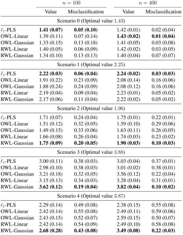
sce-narios with 5 covariates . . . 74 3.2 Mean (std) of treatment matching factors for scenarios with 5 covariates . 75 3.3 Mean (std) of empirical value functions and misclassification rates for

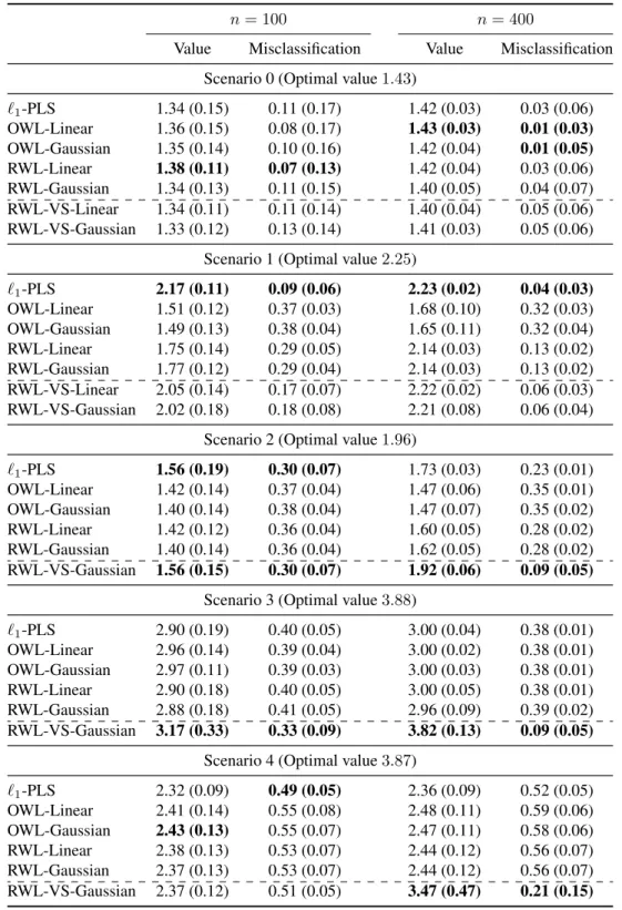
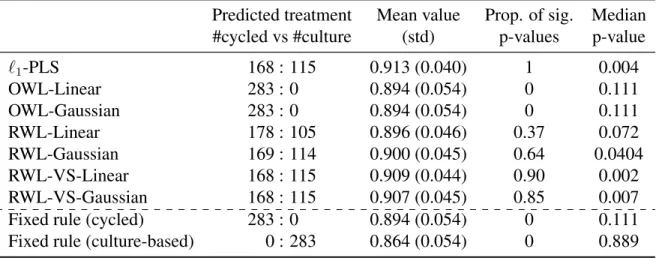
sce-narios with 50 covariates . . . 76 3.4 Comparison of methods for estimating ITR on the EPIC data with thePa

endpoint . . . 77 3.5 Comparison of methods for estimating ITR on the EPIC data with the PE

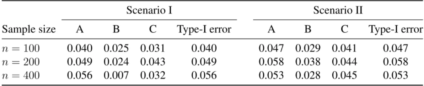
endpoint . . . 77 4.1 Proportions of significantpvalues and Type-I error rates in Scenario I and

II. . . 94 4.2 Power comparison between the permutation test and the oracle Gail-Simon

test in Scenario III and IV. . . 96 C.1 Mean (std) of empirical value functions and misclassification rates for

(10)

LIST OF FIGURES

1.1 Examples of regression-based approaches . . . 7

3.1 Example of residual weighted learning . . . 35

3.2 Loss functions . . . 38

3.3 True optimal ITRs in simulation studies . . . 58

4.1 Different types of treatment-covariate relationships. . . 90

4.2 Histograms of the null distributions on the Nefazodone-CBASP data . . . 100

(11)

CHAPTER 1: LITERATURE REVIEW

1.1 Introduction

Recently, personalized medicine has received much attention among statisticians, com-puter scientists, and clinicians. The purpose of personalized medicine is to tailor treatments to individual patient to maximize treatment benefit and safety in health care. There are al-ready some marketed tailored therapies. For example, ceritinib, a newly approved drug by FDA for the treatment of lung cancer, is highly active in patients with advanced, ALK-rearranged non-small-cell lung cancer (Shaw et al. 2014). Patients often show significant heterogeneity in response to treatments. This inherent heterogeneity suggests a transition from the traditional “one size fits all” approach to modern personalized medicine.

(12)

time to an individual.

In this dissertation, we focus on the single-stage decision problem. It is the building block for the multi-stage decision problem. Although it is a special case of dynamic treat-ment regimes, it has wider applications. Dynamic treattreat-ment regimes are mainly applicable to the chronic diseases, while optimal treatment regimes arise in almost all clinical areas.

1.2 Framework and Assumptions

For each patient, we observe a triplet(X, A, R): individual baseline covariatesX ∈ X, treatment assignmentA∈ Aand the clinical outcomeR ∈_Rwith larger values ofRbeing more desirable. We follow the convention that a random variable is indicated with a capital letter and its realization is represented by a lower-case letter.

A treatment regime dis a function of a patient’s covariates X, and outputs a value in A. The goal of optimal treatment regimes is to identify the best treatment regime dopt after observing the corresponding baseline covariates x so that the resulting outcome is optimized.

We then introduce the potential outcomes framework. The notion ofpotential outcomes (also called counterfactuals) (Robins 1986) is defined as a patient’s outcome if she had followed a particular treatment regime, possibly different from the regime that she was actually observed to follow. Mathematically, potential outcomes are

W∗ ={R∗(a) :a∈ A}, (1.1)

where R∗₍_a₎ _{is the outcome if the patient were to have been administered the treatment}

a. For a treatment regimed, define the potential outcomes associated with das{R∗₍_d_)}_.

(13)

regimedopt_{is the one satisfies}

E(R∗(d)|X =x)≤E(R∗(dopt)|X =x), ∀dand allx∈ X. (1.2) Sincexis arbitrary, (1.2) is equivalent to finding the regime withE(R∗(d))≤E(R∗(dopt)) for anyd. The quantityV(d) :=E(R∗(d))is called the value function ofd.

Potential outcomes for a given patient with a specified d are not observed. Thus we have to estimatedopt_{in (1.2) using data from a observational study or a clinical trial. The} following assumptions are required for estimation.

• Consistency assumption (Robins 1994): the potential outcomes under the observed treatment regime and the observed outcomes agree,i.e.R =R∗₍_A₎_.

• Stable unit treatment value assumption (SUTVA) (Rubin 1978): A patient’s outcome is not influenced by other patients’ treatment allocation.

• No unmeasured confounders (NUC) (Robins 1997): conditional on covariates, the treatment actually received is independent of potential outcomes. That is, for any regimea∈ A,

A⊥R∗(a)|X.

The first assumption is fundamental for the potential outcomes framework. This assump-tion requires that the outcome after a given treatment is the same, regardless of the man-ner in which treatments are ‘assigned’. The second assumption is often reasonable when patients are independently drawn from a large population. The third assumption always holds under complete or sequential randomization, and hence is also called the sequential ignorability assumption. This assumption may also hold in observational studies where all relevant confounders have been measured.

(14)

participants with covariates x have an innegligible probability of receiving any available treatment. The positivity may be violated either theoretically or practically. A theoretical violation occurs if the study design excludes certain subjects from receiving a particular treatment. For instance, in a sequential multiple assignment randomized trial (SMART) described in (Murphy 2005), the treatment options at the second stage are different for responders and non-responders to the treatments at the first stage. A practical violation of the positivity assumption occurs when a particular group of the subjects has a very low probability of receiving some treatment.

1.3 Optimal treatment regimes

Assuming that the data generating mechanism is known, the best treatment regime is dictated by the Bayes rule. In particular, to fix idea, consider the case where there are two treatment choices, that is A = {1,−1}. The potential outcomes are {R∗(1), R∗(−1)}. According to the consistency assumption,R =R∗(1)I(A= 1) +R∗(−1)I(A=−1). The NUC assumption says A⊥(R∗₍₁₎_{, R}∗_(−1))|_{X. By those assumptions, we can derive the}

conditional expected potential outcome, under any treatment regimed:X → A, as

E(R∗(d)|X =x) = _E R∗(1)|X =x

I d(x) = 1+E R∗(−1)|X =xI d(x) = −1

= E R|X =x, A= 1I d(x) = 1+E R|X =x, A=−1I d(x) = −1.

Let

Q(x, a) :=_E(R|X =x, A=a), a ∈ A, x∈ X,

(15)

Bayes rule:

dopt(x) = argmax a∈A

Q(x, a) =   

 

1 if Q(x,1)> Q(x,−1), −1 if Q(x,1)≤Q(x,−1).

(1.3)

Naturally, there are three different paradigms to approach the single-stage decision problems. The first paradigm is based on the treatment effect: first estimate the expected outcomesQ(x,1)andQ(x,−1), and plug the estimates into (1.3) to yield a treatment rule. There is a significant amount of literature developing optimal regimes based on predicting patients’ outcomes (Cai et al. 2011, Zhao et al. 2009). Recently, Qian and Murphy (2011) proposed an`1penalized least squares (`1-PLS) approach to estimate the optimal treatment

regime. Using a sparse`1 penalty to model conditional expected outcomes, this method

introduces parsimony and facilitates ease of interpretation.

The second paradigm is related to the treatment contrast function C(x) := Q(x,1)− Q(x,−1). First estimate the treatment contrast function, and assign treatment1ifC(x)> 0, and −1otherwise. For instance, Tian et al. (2012) developed a simple method using modified covariates to estimate the contrast function directly without the need for mod-elling the expected outcomes. Coupled with an efficiency augmentation procedure, this method yields clinically meaningful estimators in a variety of settings. The advantage learning (A-learning) also falls in this paradigm (Robins 2004, Murphy 2003, Moodie et al. 2007).

The first two paradigms are regression-based approaches. Their aim is to estimate the contrast function C(x). Given a sample Dn = {(Xi, Ai, Ri)n

i=1}. Let Cn(x) be an

(16)

Theorem 1.3.1. For a sequenceCn(X)of estimates forC(X), we have Vopt− V(dn)≤

p

E(Cn(X)−C(X))2,

whereVopt _:=_V₍_dopt₎_{is the optimal value function.}

Proof. For any treatment regimed, we have V(d) = E

RI(A=d(X)) P(A|X)

= E(E(R|A = 1, X)I(d(X) = 1) +E(R|A =−1, X)I(d(X) = −1))

= E(Q(X,1)I(d(X) = 1) +Q(X,−1)I(d(X) =−1)).

Thus,

Vopt− V(dn) = E((Q(X,1)−Q(X,−1))(I(dopt(X) = 1)−I(dn(X) = 1)))

= E(|C(X)|I(dopt(X)6=dn(X)))

≤ _E(|Cn(X)−C(X)|I(dopt(X)6=dn(X))).

The last inequality is from the construction ofdnanddopt_{. The desired result follows from} the Cauchy-Schwarz inequality.

Consistent regression estimation leads to consistent treatment selection. But as shown in Figure 1.1, a good treatment decision function Cn(x) does not require to be a good regression estimate ofC(x). For the optimal treatment regime problem, it is sufficient for Cn(x)to be close toC(x)only near the zeros ofC(x), and elsewhereCn(x)does not need to be close to C(x). In general, estimating the optimal treatment regime is easier than regression function estimation. Regression-based approaches are not the only way to solve the optimal treatment regime problem.

(17)

Cn(x)

C′ n(x)

x C(x)

Figure 1.1: Cn(x)andC_n0(x)are two linear estimates of the contrast functionC(x). Let dn(x) = sign(Cn(x)) and dn0(x) = sign(Cn0(x)) be their associated treatment selection rules. ThoughC0

n(x)is a poor estimate ofC(x), its associated selection rule is better than that ofCn(x).

important quantity in this paradigm is the risk function,

R(d) :=E(R|A6=d(X)) = E

R

P(A|X)I(A6=d(X))

, (1.4)

(18)

1.4 Outline of the dissertation

In this dissertation, we propose two machine learning methods to finding optimal treat-ment regimes. Chapter 2 apply thek-nearest neighbor (kNN) rule, a simple nonparametric approach. We show that thekNN rule is universally consistent, and establish its conver-gence rate. We also develop an adaptivek-nearest neighbor (AkNN) rule to perform metric selection and variable selection.

In Chapter 3, we demonstrate several weaknesses in outcome weighted learning (OWL), and then propose a general framework, called residual weighted learning (RWL), to alle-viate these problems. RWL weights misclassification errors by residuals of the outcome from a regression fit on clinical covariates excluding treatment assignments. We also pro-pose variable selection methods for linear and nonlinear rules, respectively. We show that the RWL estimator is consistent, and obtain the convergence rate.

In Chapter 4, we address an important practical issue, detecting qualitative interac-tions, in the language of optimal treatment regimes. Qualitative interactions arise when the direction of the treatment effect changes among different subsets. In this work, we estimate the optimal treatment regime by a modified residual weighted learning method, called mirrored residual weighted learning (MRWL), and then apply a permutation test to make inference on the estimated regime for We develop a permutation test for qualitative treatment-covariates interactions.

(19)

CHAPTER 2: NEAREST NEIGHBOR REGIMES

2.1 Introduction

Recently, personalized medicine has received much attention among statisticians, com-puter scientists and clinicians. The purpose of personalized medicine is to tailor treatments to individual patients to maximize treatment benefit and safety in health care. There are al-ready several marketed tailored therapies. For example, ceritinib, a recently FDA approved drug for the treatment of lung cancer, is highly active in patients with advanced, ALK-rearranged non-small-cell lung cancer (Shaw et al. 2014). Patients often show significant heterogeneity in response to treatments. This inherent heterogeneity suggests a transition from the traditional “one size fits all” approach to modern personalized medicine.

(20)

estimates.

Recently, several researchers have applied classification methods to optimal treatment regimes. For example, Zhao et al. (2012) proposed outcome weighted learning (OWL) to construct a treatment selection rule that directly optimizes the clinical outcome under this rule. They cast the treatment selection problem as a weighted classification problem, and apply state-of-the-art support vector machines to address it. Zhang et al. (2012a) also proposed a general framework to make use of classification methods to treatment regimes.

The k-nearest neighbor rule is a simple and intuitively appealing classification ap-proach, where a subject is classified by a majority vote of its neighbors. Since its con-ception in 1951 (Fix and Hodges 1951), it has attracted many researchers, and retains its popularity today (Cover and Hart 1967, Stone 1977, Gy¨orfi 1981, Devroye and Gy¨orfi 1985, Hastie and Tibshirani 1996, Domeniconi et al. 2002, Lindenbaum et al. 2004, Atiya 2005, Hall et al. 2008, Biau et al. 2010, Samworth 2012). The rationale of nearest neighbor rules is that close covariate vectors share similar properties more often than not.

In this article, we propose a k-nearest neighbor (kNN) rule for optimal treatment regimes. Although the rule is simple, it possesses good theoretical properties. Firstly, we show that the kNN rule for optimal treatment regimes is universally consistent. The notion of universal consistency is borrowed from machine learning. In optimal treatment regimes, it requires for a rule that when the sample size approaches infinity the rule eventu-ally learns the Bayes rule without knowing any specifics about the distribution of the data. Secondly, we establish its convergence rate. The convergence rate is as high asn−1/2 _with

appropriately chosenkif the dimension of covariates is 1 or 2, and the rate isn−2/(p+2)_for

dimensionalityp≥3.

(21)

alleviate this problem, we propose an adaptivek-nearest neighbor (AkNN) rule, where the distance metric is adaptively determined from the data. Through adaptive metric selection, AkNN performs variable selection implicitly. The superior performance of AkNN over kNN is illustrated in the simulation studies. Actually, the kNN rule is a special case of AkNN. In practical settings, we recommend AkNN.

The remainder of the article is organized as follows. In Section 2.2, we propose the kNN rule for optimal treatment regimes, establish its theoretical properties, and improve the rule through an adaptive procedure. We present simulation studies to evaluate per-formance of the proposed methods in Section 2.3. The method is then illustrated on the Nefazodone-CBASP clinical trial (Keller et al. 2000) in Section 2.4. We conclude the article with a discussion in Section 2.5. Theoretical proofs are given in the Appendix.

2.2 Methods

2.2.1 Nearest neighbor rules

Consider a randomized clinical trial with L treatment arms. We observe a triplet (X, A, R) from each patient, where X = (X1,· · · , Xp)T ∈ Rp denotes the patient’s

clinical covariates,A∈ A={1,2,· · · , L}denotes the treatment assignment, andR∈ R is the observed clinical outcome. Assume without loss of generality that larger values of R are preferred. Let π`(x) := P(A = `|X = x) be the probability of being assigned treatment ` for a patient with clinical covariatesx. This probability is predefined in the trial design.

(22)

expected value ofR given that the regimedis applied to the given population of patients. There is a positivity assumption that π`(X) > 0 for any ` ∈ A. That is, any treatment option must be represented in the data in order to estimate an optimal regime. An optimal treatment regime d∗ _{is a regime that maximizes} _V(_d₎_{. The regime} _d∗ _{is also called the}

Bayes rule. For simplicity, letm`(x) := E(R|X =x, A = `). Because of the positivity assumption,m`(x)is well defined. It is easy to obtain that

d∗(x) = argmax `∈{1,···,L}

m`(x). (2.1)

Thek-nearest neighbor rule is a nonparametric method used for classification and re-gression (Fix and Hodges 1951). In this article, we apply the nearest neighbor rule to optimal treatment regimes. The idea is simple. We use the nearest neighbor algorithm to estimate the conditional outcomem`(x)for each arm, and plug into (2.1) to get the nearest neighbor estimate for the optimal treatment regime.

Assume that the observed data Dn = {(Xi, Ai, Ri) : i = 1,· · · , n} are collected independently. We fixx∈ _Rp_{, and reorder the observed data}_Dn_{according to increasing} values of||Xi−x||. The reordered data sequence is denoted by

X(1,n)(x), A(1,n)(x), R(1,n)(x)

,· · · ,X(n,n)(x), A(n,n)(x), R(n,n)(x)

.

ThusX(1,n)(x),· · · ,X(k,n)(x)are k nearest neighbors ofx. When the k-nearest

neigh-borhood ofxis small, its conditional outcome for arm`can be estimated by

b

m`(x) = Pk

i=1R(i,n)(x)

I(A(i,n)(x)=`)

π`(X(i,n)(x))

Pk i=1

I(A(i,n)(x)=`)

π`(X(i,n)(x))

,

where_I(·)is the indicator function, as suggested in Murphy (2005). Here we define0/0 = 0. For simplicity, denote

W_n,i` (x) =     

   

I(A₍_i,n₎₍x)=`)

π`(X₍_i,n₎₍x))

Pk

j=1

I(A₍_j,n₎₍x)=`)

π`(X₍_j,n₎₍x))

, if i≤k,

(23)

Thek-nearest neighbor estimatem_b` can now be rewritten as,

b

m`(x) = n X

i=1

W_n,i` (x)R(i,n)(x). (2.2)

Thus the plug-in estimate of the Bayes rule in (2.1) is dN N(x) = argmax

`∈{1,···,L} b

m`(x). (2.3)

This is called thek-nearest neighbor regime, for shortkNN, in this article.

We need to address the problem of distance ties,i.e., when||x−Xi||=||x−Xj||for somei 6= j. Devroye et al. (1996, Section 11.2) discussed several methods for breaking distance ties. In practical use, we adopt the tie-breaking method used in Stone (1977). Subjects who have the same distance fromxas thek-th nearest neighbor are averaged on the outcome R. We denote the distance of the k-th nearest neighbor to x by ρn(x), and define the setsAn(x) := {i:||x−Xi||< ρn(x)}andBn(x) :={i:||x−Xi||=ρn(x)}. The revised rule of (2.2) is as follows:

e

m`(x) = P

i∈An(x)R(i,n)(x)

I(A(i,n)(x)=`)

π`(X(i,n)(x)) +

k−|An(x)| |Bn(x)|

P

i∈Bn(x)R(i,n)(x)

I(A(i,n)(x)=`)

π`(X(i,n)(x))

P i∈An(x)

I(A(i,n)(x)=`)

π`(X(i,n)(x)) +

k−|An(x)| |Bn(x)|

P i∈Bn(x)

I(A(i,n)(x)=`)

π`(X(i,n)(x))

.

(2.4) The corresponding nearest neighbor regime is the regime in (2.3) obtained by replacing

b

m`(x)withm`_e (x). This is not a strictlyk-nearest neighbor rule when there are distance ties on thek-th nearest neighbor, since the estimate uses more thankneighbors.

(24)

other parts, and obtain the predicted treatment for each patient. The cross-validated value function is given by Pn[RI(A = P red)/πA(X)]/Pn[I(A = P red)/πA(X)], where Pn denotes the empirical average andP red is the predicted treatment in the cross validation procedure. In this article, we apply 10-fold cross validation to tune the parameterk.

2.2.2 Theoretical Properties

In the literature of machine learning, a classification rule is called universally consistent if its expected error probability converges to the Bayes error probability, in probability or almost surely, for all distributions underlying the data (Devroye et al. 1996). Although this generality in distribution may seem to be a very strong condition, it has been known since a seminal paper by Stone (1977) that there do exist such classification rules. The k-nearest neighbor classification is the first to be proved to possess such universal consistency (Stone 1977, Devroye et al. 1996). Here, we extend the concept of universal consistency to optimal treatment regimes.

Definition 2.2.1. Given a sequenceDnof data, an optimal treatment regimednis univer-sally (weakly) consistent if

lim

n→∞V(dn) = V(d

∗₎ _{in probability}

for all probability measuresP on_Rp × A × R, and universally strongly consistent if lim

n→∞V(dn) = V(d

∗₎ _{almost surely}

for all probability measuresP on_Rp × A × R.

(25)

Before proceeding to the theoretical analysis, we need some definitions. Denote the probability measure for X by µ, and let Sx, be the closed ball centered at x of radius > 0. The collection of all xwith µ(Sx,) > 0 for all > 0 is called the support ofµ (Cover and Hart 1967). The set is denoted assupport(µ).

The analysis of universal consistency requires some assumptions:

(A1) There exists a constants ζ > 0 such thatπ`(x) ≥ ζ for any x ∈ support(µ) and `∈ {1,· · · , L}.

(A2) _E|R|<∞.

(A3) Distance ties occur with probability zero inµ.

These assumptions are quite weak. Assumption (A1) is just the positivity assumption, and ζ can be obtained by design. Assumption (A2) is natural. This assumption is au-tomatically satisfied for bounded outcomes, i.e. |R| ≤ M < ∞ for some constant M. Assumption (A3) is to avoid the messy problem of distance ties. When (A3) does not hold, we may add a small uniform variable U ∼ unif orm[0, ] independent of (X, A, R) to the vector X. This causes the (p+ 1)-dimensional random vector X0 = (X, U)to sat-isfy Assumption (A3). We may perform thek-nearest neighbor rule on the modified data D0

n ={(Xi0, Ai, Ri) : i = 1,· · · , n}. Because of the independence ofU, the correspond-ing conditional outcomem0

(26)

The following theorem shows universal consistency of the nearest neighbor regime. The proof is provided in the Appendix.

Theorem 2.2.1. For any distributionP for(X, A, R)satisfying assumptions (A1)∼(A3),

(i) thekNN regime in (2.3) is universally weakly consistent ifk → ∞andk/n→0;

(ii) the kNN regime in (2.3) is universally strongly consistent if k/log(n) → ∞ and k/n→0.

If Assumption (A2) is tightened to |R| ≤ M < ∞ for some constant M, the kNN regime in (2.3) is universally strongly consistent ifk→ ∞andk/n→0.

The next natural question is whether the associated value of thekNN regime tends to the Bayes value at a specified rate. To establish the rate of convergence, we require stronger assumptions.

(A10) Pn_i₌₁W`

n,i(x) = 1for all x ∈ Rp and ` = 1,· · · , L; and there exists a constantc such thatW`

n,i(x)≤c/kfor allx∈Rp,i= 1,· · · , nand` = 1,· · · , L. (A20) There exists a constantσ2 _{such that}_σ2

`(x) := V ar(R|X = x, A =`)≤ σ2 for all x∈_Rp_and_`_{= 1}_,_{· · ·} _{, L.}

(A30) Distance ties occur with probability zero inµ, and the support ofµis compact with diameter2ρ.

(A40) m`’s are Lipschitz continuous,i.e., there exists a constantC >0such that|m`(x)− m`(x0)| ≤C||x−x0||for anyxandx0inRp, and` = 1,· · · , L.

(27)

Theorem 2.2.2. For any distributionP for(X, A, R)satisfying assumptions (A10)∼(A40), there exists a sequencek such thatk → ∞andk/n→0, and

E n

V(d∗)− V(dN N)2o

=O(n−β).

When p = 1, β = 1/2; when p = 2, β can be arbitrarily close to 1/2; when p ≥ 3, β = 2/(p+ 2).

The rate of convergence is as high as n−1/2 _{if dimensionality} _p _{is 1 or 2. When} _p

increases, the convergence rate decreases significantly. As with nearest neighbor rules in classification and regression, thekNN regime also suffers from the curse of dimensionality.

2.2.3 Adaptive rule

Determination of nearest neighbors highly depends on the distance metric. Thus the performance of the kNN regime is affected by metric selection. The nearest neighbor regime is consistent as shown previously. However, it is well known that the curse of dimensionality can severely hurt nearest neighbor rules in finite samples. The rate of convergence in Theorem 2.2.2 is slow when dimensionality is high. Hence appropriate variable selection may improve performance. In this section, we propose an adaptive k-nearest neighbor algorithm to estimate the optimal treatment regime, and to perform metric selection and variable selection simultaneously.

Let Σ = diag(σ2

1,· · · , σ2p) be a diagonal matrix, and use the quadratic form (x1 − x2)TΣ(x1 −x2)to compute the (squared) distance betweenx1 andx2. σj is the scaling

factor for thej-th covariate. Settingσj = 0 is equivalent to discarding thej-th covariate. We intend to set a largeσ2

j if thej-th covariate is important for treatment selection.

(28)

dj_{only involves the}_{j-th covariate, and the other}_d0_{, called non-informative regime, assigns}

all patients to the treatment with the largest estimated conditional outcomeEb(R|A=`) := Pn

i=1

RiI(Ai=`)

π`(Xi) /

Pn i=1

I(Ai=`)

π`(Xi). For a specific regime d, letdi be the treatment assignment

for thei-th subject according tod. The value function associated withdis estimated by

b V(d) =

Pn i=1Ri

I(Ai=di)

π_Ai(Xi)

Pn i=1

I(Ai=di)

π_Ai(Xi)

. (2.5)

When we compare two treatment regimes,dj _and_d0_{, a consistent estimator of the variance}

of√n(V(b dj)−Vb(d0))is

d

V ar√n(Vb(dj)−V(b d0)) = 1 n n X i=1   

I(Ai =dji) πAi(Xi)

(Ri −Vb(dj)) !2

+

I(Ai =d0i) πAi(Xi)

(Ri−V(b d0)) 2

 

 .(2.6)

Note that even ifdj _{only depends on one single covariate, or}_d0_{is not related to any}

covari-ate,πAi(Xi)in (2.5) and (2.6) is still based on the whole covariate vector by design. The

statistic

Tj =

√

n(V(b dj)−V(b d0)) r

d

V ar√n(Vb(dj)−V(b d0))

(2.7)

asymptotically has a standard normal distribution under the null hypothesis thatV(dj_{) =} V(d0₎_{. See Murphy (2005) for technical details. When the statistic is greater than zero,}

regimedj _{is considered better than the non-informative regime} _d0_{, otherwise}_d0 _{is better.}

The statisticTj reflects the importance of thej-th covariate on optimal treatment regimes. We estimatedj bykNN only using thej-th covariate. The parameterkis tuned by 10-fold cross validation. The treatment assignments,dj_i’s, are also obtained by cross validation to avoid over-fitting.

We setσ2

j = (Tj+ ∆)+for eachj = 1,· · · , p, where∆∈Ris a predefined parameter

and (·)+ is the positive part. The adaptive k-nearest neighbor regime, denoted AkNN,

(29)

uses an adaptive distance metric(x1−x2)TΣ(x1−x2)to compute the (squared) distance

betweenx1andx2. When∆is small (for example,∆→ −∞), all theσj2’s are zero, hence the AkNN regime degenerates to a non-informative regime. On the other hand, when ∆ is large (for example,∆→ ∞), all theσ2

j’s are almost identical, and the AkNN regime is equivalent to thekNN one.

Here is a summary of the adaptive nearest neighbor procedure:

1) Normalize each covariate to a similar scale.

2) CalculateTj in (2.7) for each covariatej = 1,· · · , p. 3) CalculateΣ =diag(σ2

1,· · · , σp2), whereσj2 = (Tj+ ∆)+.

4) Estimate akNN regime using the distance metric, d(x1,x2) =

p

(x1−x2)TΣ(x1−x2).

The scaling at the first step is to avoid covariates in greater numeric ranges dominating those in smaller numeric ranges. We recommend linearly scaling each covariate to the range[−1,+1] or[0,1](Hsu et al. 2003). For AkNN, there are two tuning parameters,k and∆. We tune the parameters using 10-fold cross validation as done previously.

2.3 Simulation studies

We carried out extensive simulation studies to investigate finite sample performance of the proposedkNN and AkNN methods. In the simulations, we generated 10-dimensional vectors of clinical covariatesx1,· · · , x10, consisting of independent uniform random

vari-ables U(−1,1). The treatmentA was generated from {−1,1} independently of X with P(A = 1) = 0.5. The response R was normally distributed with mean Q0 = µ0(x) +

(30)

andδ0(x)·ais the interaction between treatment and clinical covariates. We considered

three scenarios with different choices ofµ0(x)andδ0(x):

(1) µ0(x) = 1 +x1+x2+ 2x3+ 0.5x4; δ0(x) = 1.8(0.3−x1 −x2).

(2) µ0(x) = 1 +x21+x22+ 2x23; δ0(x) = 10(1−x21−x22)(x12+x22−0.2).

(3) µ0(x) = 1 +x21+x22+ 2x23; δ0(x) = 5(1−

P10

i=1

x2

i

i ).

The scenarios have different true decision boundaries. The decision boundaries in the first two scenarios are determined byx1andx2only. The decision boundary is a line in Scenario

1 and a ring in Scenario 2. The decision boundary in Scenario 3 is a sphere in_R10, while the first several covariates play an important role in the regime.

We compared the performance of the following five methods: (1) The proposedkNN method; (2) The proposed AkNN method; (3) OWL proposed in Zhao et al. (2012) us-ing the Gaussian RBF kernel Gaussian); (4) OWL usus-ing the linear kernel (OWL-Linear); and (5)`1-PLS proposed by Qian and Murphy (2011).

OWL methods view the optimal treatment regime problem as a weighted classification problem, and treat the original outcomes as weights. OWL-Linear incorporates the linear kernel to estimate linear treatment regimes, while OWL-Gaussian has the ability to de-tect nonlinear regimes. Since OWL methods can only handle nonnegative outcomes, we subtractedmin{Ri}from all outcome responses. This is the approach used in Zhao et al. (2012) [personal communication].`1-PLS is a two-step method. In the simulation studies,

`1-PLS approximatedE(R|X, A)using the basis function set(1,X, A,XA), and applied

LASSO for variable selection. The optimal treatment regime was determined by the sign of the difference between the estimated_E(R|X, A= 1)and_E(R|X, A=−1).

(31)

tuning parameter. In the simulations, we applied 10-fold cross validation to tune param-eters. For comparison, the performances of the five methods were evaluated by the value function under the estimated optimal treatment regime when applied to an independent and large test dataset. Specifically, a test set with 10,000 observations was simulated to assess the performance. The estimated value function under any regime d is given by P∗n[RI(A = d(X))/πA(X)]/P∗n[I(A = d(X))/πA(X)] (Murphy 2005), where P∗n de-notes the empirical average using the test data.

The simulation results are presented in Table 2.1. We report the mean and standard deviation of value functions over 500 replications. Scenario 1 was a linear example. The model specification in `1-PLS was correct, and this method performed very well. kNN

showed better performance than both OWL methods. AkNN further improved the perfor-mance of kNN, and yielded similar performance to `1-PLS especially when the sample

size is large. The conditional mean outcomes and decision boundaries in the remaining two scenarios were nonlinear.`1-PLS and OWL-Linear were misspecified, and hence they

did not perform very well in either scenarios. We focused on the comparison among OWL-Gaussian,kNN and AkNN. In Scenario 2, either OWL-Gaussian orkNN did not perform better than`1-PLS or OWL-Linear, even though they can detect nonlinear decision

bound-ary. The poor performance is probably due to noise covariates. It is well known that nearest neighbor rules deteriorate when there are irrelevant covariates presented in the data. Due to the variable selection mechanism with AkNN, this method outperformed other methods in terms of achieving much higher values. Scenario 3 was an example where all covariates contributed to the optimal treatment regime. However, their level of contribution varied. The first covariate was the most important, while the tenth was the least. In this scenario, kNN and OWL-Gaussian showed better performance than both OWL-Linear and`1-PLS.

(32)

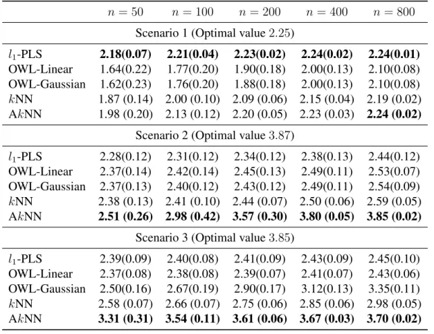
Table 2.1:Mean (std) of empirical value function for three simulation scenarios evaluated on independent validation data. The best value function for each scenario and sample size combination is in bold.

n= 50 n= 100 n= 200 n= 400 n= 800

Scenario 1 (Optimal value2.25)

l1-PLS 2.18(0.07) 2.21(0.04) 2.23(0.02) 2.24(0.02) 2.24(0.01)

OWL-Linear 1.64(0.22) 1.77(0.20) 1.90(0.18) 2.00(0.13) 2.10(0.08) OWL-Gaussian 1.62(0.23) 1.76(0.20) 1.88(0.18) 2.00(0.13) 2.10(0.08) kNN 1.87 (0.14) 2.00 (0.10) 2.09 (0.06) 2.15 (0.04) 2.19 (0.02) AkNN 1.98 (0.20) 2.13 (0.12) 2.20 (0.05) 2.23 (0.03) 2.24 (0.02)

l1-PLS 2.28(0.12) 2.31(0.12) 2.34(0.12) 2.38(0.13) 2.44(0.12)

l1-PLS 2.39(0.09) 2.40(0.08) 2.41(0.09) 2.43(0.09) 2.45(0.10)

equivalent tokNN. Considering the superior performance of AkNN overkNN, we suggest AkNN for general practical use.

2.4 Data analysis

(33)

Nefazodone and CBASP (COMB). The primary outcome measurement in efficacy was the score on the 24-item Hamilton Rating Scale for Depression (HRSD). Lower HRSD is de-sirable. We considered 50 pre-treatment covariates as in Zhao et al. (2012). We excluded some patients with missing covariate values from the analyses. The data used here con-sisted of 647 patients. Among them, 216, 220, and 211 patients were assigned to NFZ, CBASP and COMB, respectively. Each clinical covariate was linearly scaled to the range [−1,+1], as recommended in Hsu et al. (2003).

Since the trial had three treatment arms, we compared the performance of AkNN with l1-PLS. The OWL methods can only deal with two treatments. From the simulation studies,

AkNN always outperformskNN, so we only considered AkNN in this section. Outcomes used in the analyses were opposites of the HRSD scores. l1-PLS used the basis function

(34)

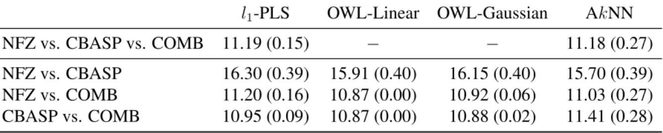
Table 2.2: Mean (std) Hamilton rating scale for depression (HRSD) from the cross-validation procedure using different methods. Lower HRSD is better.

l1-PLS OWL-Linear OWL-Gaussian AkNN

NFZ vs. CBASP vs. COMB 11.19 (0.15) − − 11.18 (0.27)

NFZ vs. CBASP 16.30 (0.39) 15.91 (0.40) 16.15 (0.40) 15.70 (0.39) NFZ vs. COMB 11.20 (0.16) 10.87 (0.00) 10.92 (0.06) 11.03 (0.27) CBASP vs. COMB 10.95 (0.09) 10.87 (0.00) 10.88 (0.02) 11.41 (0.28)

patients. The original analysis in Keller et al. (2000) indicated that the combination of Nefazodone and CBASP (COMB) is significantly more efficacious than either treatment alone. Our analysis confirmed this is indeed true.

(35)

2.5 Discussion

In this article, we have proposed a simplekNN rule for optimal treatment regimes, and developed an adaptive method (AkNN) to determine the distance metric. As shown in the simulation and data studies, the simple method can rival and improve upon sophisticated methods. The proposed methods are easy to implement. We have implemented them using an R packageFNN, which utilizes fastk-nearest neighbor search algorithms, such as cover tree (Beygelzimer et al. 2006) and k-d tree (Friedman et al. 1977), to speed up the brute force search. Our nearest neighbor algorithms can be fast even for data with a large sample size.

The proposed methods are nonparametric. According to universal consistency, kNN will eventually learn the optimal treatment regime as the sample size increases. Two-step methods, such as`1-PLS, are generally parametric. Their performance mainly depends on

(36)

CHAPTER 3: RESIDUAL WEIGHTED LEARNING

3.1 Introduction

Personalized medicine is a medical paradigm that utilizes individual patient informa-tion to optimize patients health care. Recently, personalized medicine has received much attention among statisticians, computer scientists, and clinical practitioners. The primary motivation is the well-established fact that patients often show significant heterogeneity in response to treatments. For instance, in a recent study, it was demonstrated that the optimal timing for the initiation of antiretroviral therapy (ART) varies in patients co-infected with human immunodeficiency virus and tuberculosis. Patients with CD4+ T-cell counts of less than 50 per cubic millimeter benefited substantially from earlier ART with a lower rate of new AIDS-defining illnesses and mortality as compared with later ART, while those with larger CD4+ T-cell counts did not have such a benefit (Havlir et al. 2011). The inherent heterogeneity across patients suggests a transition from the traditional “one size fits all” approach to modern personalized medicine.

(37)

indi-rectly by inverting the regression estimates instead of diindi-rectly optimizing the decision rule. For instance, Qian and Murphy (2011) applied a two-step procedure that first estimates a conditional mean for the outcome and then determines the treatment rule by comparing the conditional means across various treatments. The success of these indirect approaches highly depends on correct specification of posited models and on the precision of model estimates.

In contrast, Zhao et al. (2012) proposed outcome weighted learning (OWL), using data from a randomized clinical trial, to construct an ITR that directly optimizes the clinical out-come. They cast the treatment selection problem as a weighted classification problem, and apply state-of-the-art support vector machines for implementation. This approach opens the door to introducing machine learning techniques into this area. However, there is still significant room for improved performance. First, the estimated ITR of OWL is affected by a simple shift of the outcome. This behavior makes the estimate of OWL unstable. Sec-ond, since OWL requires the outcome to be nonnegative, OWL works similarly to weighted classification, in which misclassification errors, the differences between the estimated and true treatment assignments, are targeted to be reduced. Hence the ITR estimated by OWL tries to keep treatment assignments that subjects actually received. This is not always ideal since treatments are randomly assigned in the trial, and the probability is slim that the majority of subjects are assigned optimal treatments. Third, OWL does not have variable selection features. When there are many clinical covariates which are not related to the heterogeneous treatment effects, variable selection is critical to the performance.

(38)

some residuals are negative, the hinge loss function used in OWL is not appropriate. We instead utilize the smoothed ramp loss function, and provide a difference of convex (d.c.) algorithm to solve the corresponding non-convex optimization problem. The smoothed ramp loss resembles the ramp loss (Collobert et al. 2006), but it is smooth everywhere. It is well known that ramp loss related methods are shown to be robust to outliers (Wu and Liu 2007). The robustness to outliers for the smoothed ramp loss is helpful for RWL, especially when residuals are poorly estimated. Moreover, through using residuals, RWL is able to deal relatively easily with almost all types of outcomes. For example, RWL can work with generalized linear models to construct ITRs for count/rate outcomes. We also propose variable selection approaches in RWL for linear and nonlinear rules, respectively, to further improve finite sample performance.

The theoretical analysis of RWL focuses on two aspects, universal consistency and convergence rate. The notion of universal consistency is borrowed from machine learning. It requires for a learning method that when the sample size approaches infinity the method eventually learns the Bayes rule without knowing any specifics of the distribution of the data. We show that RWL with a universal kernel (e.g. Gaussian RBF kernel) is universally consistent. In machine learning, there is a famous “no-free-lunch theorem”, which states that the convergence rate of any particular learning rule may be arbitrarily slow (Devroye et al. 1996). In this work, we prove the “no-free-lunch theorem” for finding ITRs. Thus the rate of convergence studies for a particular rule must necessarily be accompanied by conditions on the distribution of the data. For RWL with Gaussian RBF kernel, we show that under the geometric noise condition (Steinwart and Scovel 2007) the convergence rate is as high asn−1/3_.

(39)

to reduce the variability introduced by the original outcomes. Second, since the numbers of subjects with positive and negative residuals are generally balanced, the ITR determined by RWL favors neither the treatment assignments that subjects actually received nor their opposites. Because of the above reasons, RWL improves finite sample performance. Third, RWL possesses location-scale invariance with respect to the original outcomes. Specifi-cally, the estimated rule of RWL is invariant to a shift of the outcome; it is invariant to a scaling of the outcome with a positive number; the rule from RWL that maximizes the outcome is opposite to the rule that minimizes the outcome. These are intuitively sensible.

The contributions of this work are summarized as follows. (1) We propose the general framework of Residual Weighted Learning to estimate individualized treatment rules. By estimating residuals with linear or generalized linear models, RWL can effectively deal with different types of outcomes, such as continuous, binary and count outcomes. For censored survival outcomes, RWL could potentially utilize martingale residuals, although theoretical justification is still under development. (2) We develop variable selection tech-niques in RWL to further improve performance. (3) We present a comprehensive theoreti-cal analysis of RWL on universal consistency and convergence rate. (4) As a by-product, we show the “no-free-lunch theorem” for ITRs that the convergence rate of any particular rule may be arbitrarily slow. This is a generic result, and it applies to any algorithm for optimal treatment regimes.

(40)

Section 3.5. The method is then illustrated on the EPIC cystic fibrosis randomized clinical trial (Treggiari et al. 2009; 2011) in Section 3.6. We conclude with a discussion in Section 3.7. All proofs are given in Appendix.

3.2 Methodology

3.2.1 Outcome Weighted Learning

Consider a two-arm randomized trial. We observe a triplet (X, A, R) from each pa-tient, where X = (X1,· · · , Xp)T ∈ X denotes the patient’s clinical covariates, A ∈ A = {1,−1}denotes the treatment assignment, and R is the observed clinical outcome, also called the “reward” in the literature on reinforcement learning. We assume that R is bounded, and larger values of R are more desirable. An individualized treatment rule (ITR) is a function from X to A. Let π(a,x) := P(A = a|X = x) be the probability of being assigned treatment a for patients with clinical covariates x. It is predefined in the trial design. Here we consider a general situation. In most clinical trials, the treatment assignment is independent ofX, but in some designs, such as stratified designs, A may depend onX. We assumeπ(a,x)>0for alla∈ Aandx∈ X.

An optimal ITR is a rule that maximizes the expected outcome under this rule. Mathe-matically, the expected outcome under any ITRdis given as

E(R|A=d(X)) =E

R π(A,X)I

A =d(X)

, (3.1)

(41)

is equivalent to the following minimization problem: d∗ ∈arg min

d E

R π(A,X)I

A6=d(X)

. (3.2)

Zhao et al. (2012) viewed this as a weighted classification problem, in which one wants to classifyAusingX but also weights each misclassification error byR/π(A,X).

Assume that the observed data{(xi, ai, ri) :i= 1,· · · , n}are collected independently. For any decision function f(x), let df(x) = sign f(x)

be the associated rule, where sign(u) = 1foru >0and−1otherwise. The particular choice of the value ofsign(0)is not important. In this work, we fixsign(0) =−1. Using the observed data, the weighted classification error in (3.2) can be approximated by the empirical risk

1 n

n X

i=1

ri π(ai,xi)I

df(xi)6=ai

. (3.3)

The optimal decision functionfb(x)is the one that minimizes the outcome weighted error (3.3).

It is well known that empirical risk minimization for a classification problem with the 0-1 loss function is an NP-hard problem. To alleviate this difficulty, one often finds a surrogate loss to replace the 0-1 loss. Outcome weighted learning (OWL) proposed by Zhao et al. (2012) uses the hinge loss function, and also applies the regularization technique used in the support vector machine (SVM) (Vapnik 1998). In other words, instead of minimizing (3.3), OWL aims to minimize

1 n

n X

i=1

ri π(ai,xi)

1−aif(xi)

++λ||f|| 2

, (3.4)

where(u)+ = max(u,0)is the positive part ofu,||f||is some norm forf, andλis a tuning

parameter controlling the trade-off between empirical risk and complexity of the decision functionf.

(42)

should not affect the optimal decision rule, as seen from (3.1) and (3.2). That is, d∗ _in

(3.2) does not change ifRis replaced byR+c, for any constantc. Unfortunately this nice invariance property does not hold for the decision function fb(x) of OWL in (3.4) when ri is replaced byri +c. Consider an extreme case where cis very large and π(1,x) = π(−1,x) = 0.5 for all x ∈ X, the weights (ri +c)/π(ai,xi) are almost identical, and the weighted problem is approximately transformed to an unweighted one. Hence the performance of OWL can be affected by a simple shift ofR. Second, OWL further assumes thatRis nonnegative to gain computational efficiency from convex programming. A direct consequence of this assumption, as seen from (3.3), is that the treatment regime df(xi) tends to match the treatmentai that was actually assigned to the patient, especially when the decision functionf is chosen from a rich class of functions. This property is not ideal for data from a randomized clinical trial, since treatments are actually randomly assigned to patients.

3.2.2 Residual Weighted Learning

In this section, we only consider the case that the outcomeRis continuous, and extend the framework to other types of outcomes in Section 3.2.4.

As demonstrated previously, the decision rule in (3.2) is invariant to a shift of outcome Rby any constant. Moreover, Lemma 3.2.1 shows thatd∗_{in (3.2) is invariant under a shift}

of R by a function ofX. That is,d∗ _{remains unchanged if} _R _{is replaced by} _R₋_g_(X)

(43)

to the performance of OWL. Zhao et al. (2012) did not delve deeply into this problem. In this work, we will provide a solution to this, and improve finite sample performance. Lemma 3.2.1. For any measurable g : X → _R and any probability distribution for (X, A, R),

E

R−g(X)

π(A,X) I A 6=d(X)

=_E

R

π(A,X)I A6=d(X)

−_E(g(X)).

Intuitively, the function g with the smallest variance of R−g(X)

π(A,X) I A 6= d(X)

is a good choice. However, such a function depends on the decision rule d, as shown in the following theorem. The proof of the theorem is provided in Appendix.

Theorem 3.2.1. Among all measurableg :X → _R,_eg(X) =E

R

π(A,X)I A6=d(X)

X

is the functiong that minimizes the variance of R−g(X)

π(A,X) I A6=d(X)

.

Our purpose is to find a functiong, which is not related tod, to reduce the variance of R−g(X)

π(A,X) I A6=d(X)

as much as possible. As shown in the proof, the minimizer_egcan be written as,

e

g(X) =E(R|X, A= 1)I d(X)6= 1+E(R|X, A=−1)I d(X)6=−1.

That is, _eg(X) jumps between _E(R|X, A = 1) and _E(R|X, A = −1) as d(X) varies. Hence whendis unknown, a reasonable choice ofg is

g∗(X) = E(R|X, A= 1) +E(R|X, A=−1)

2 =E

R

2π(A,X)|X

. (3.5)

We propose to minimize the following empirical risk, rather than the original one in (3.3): 1

n n X

i=1

ri −g_b∗(xi) π(ai,xi) I

df(xi)6=ai

, (3.6)

(44)

and instead we weight them by residuals from a regression fit of outcomes. Thus the opti-mal decision function is invariant under any translation of clinical outcomes. We call the method Residual Weighted Learning (RWL).

RWL also has the following interpretation. The outcomeRcan be characterized as

R =µ(X) +δ(X)·A+,

whereis the mean zero random error. µ(X)reflects common effects of clinical covariates Xfor both treatment arms. It is easy to see thatµ(X) = (_E(R|X, A= 1) +_E(R|X, A= −1))/2, so the residual, R − g∗_(X)_{, in RWL is just} _δ_(X) _·_A ₊_{, which captures all}

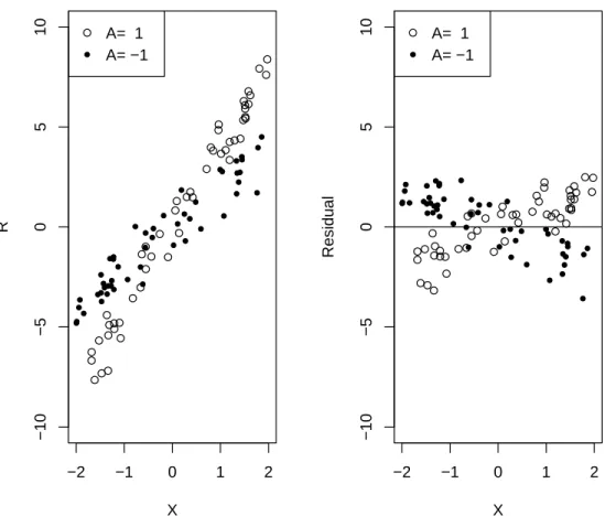
sources of heterogeneous treatment effects. The rationale of optimal treatment regimes is to keep treatment assignments that subjects have actually received if those subjects are ob-served to have large outcomes, and to switch assignments if outcomes are small. However, the largeness and smallness for outcomes are relative. A rather large outcome may still be considered as small when compared with subjects having similar clinical covariates, as shown in Figure 3.1. Outcomes are not comparable among subjects with different clinical covariates, while the residual, by removing common covariates effects, is a better measure-ment. Figure 3.1 illustrates how residuals work using an example with a single covariate X. The raw data are shown on the left, and residuals are shown on the right. Residuals are comparable among subjects, and larger residuals represent better outcomes.

(45)

−2 −1 0 1 2 −10 −5 0 5 10 X R

A= 1 A= −1

−2 −1 0 1 2

−10 −5 0 5 10 X Residual

A= 1 A= −1

Figure 3.1: Example of residual weighted learning. The raw data are shown on the left, consisting of a single covariate X, treatment assignment A = 1 or −1, and continuous outcome R with E(R|X, A) = 3X +XA. The allocation ratio is 1:1. The residuals, R−3X, are shown on the right.

estimator of (3.1) is,

1 n n X i=1 ri π(ai,xi)I

d(xi) = ai

. (3.7)

Though it is unbiased, it may give an estimate outside the range of R. While for finite samples a better estimator of (3.1) as shown in Murphy (2005) is,

1

n Pn

i=1

riI d(xi)=ai

π(ai,xi)

1

n Pn

i=1

I d(xi)=ai

π(ai,xi)

. (3.8)

The denominator is an estimator of_E

I A=d(X)

π(A,X)

(46)

proof of Lemma 3.2.1 yields _E

I A=d(X)

π(A,X)

= 1. The estimator _n1Pn_i₌₁I d(xi)=ai

π(ai,xi) is

called the treatment matching factor in this work. The factor varies between 0 and 2. If a rule favors treatment assignments that subjects have actually received, its treatment matching factor is greater than 1, while in contrast if a rule prefers the opposite treatment assignments, its treatment matching factor is less than 1. For a randomized clinical trial, we expect that the estimated rule is associated with a treatment matching factor close to 1. For OWL, since all the weights are nonnegative, the estimated rule of OWL tends to keep, if possible, the treatments that subjects actually received. Thus the associated treatment matching factor would be greater than 1, especially when the sample size is small, or when a complicated rule is applied. Hence the estimator in (3.8) might not be large even though (3.7) is maximized. RWL alleviates this problem by using residuals to make an initial guess on the optimal rule. Owing to the balance between subjects with positive and negative residuals, RWL implicitly finds a rule with its treatment matching factor close to 1.

There are many ways to estimateg∗. In this work, we consider two models. The first one is the main effects model. Assume that _E

R

2π(A,X)|X

= β0 + XTβ, where β = (β1,· · · , βp)T. The estimates βb andβb₀ can be obtained by minimizing the sum of weighted squares,

n X

i=1 1 2π(ai,xi)

(ri−β0−xTi β)2.

It can be solved easily by almost any statistical software. Then the estimate is _bg∗_{(x) =}

b

β0+xTβb. The second is the null model. Assume thatE

R

2π(A,X)|X

=β0. It is easy

to obtain_bg∗_{(x) =}_β_b

0 =Pn_i=1

ri

π(ai,xi)/

Pn i=1

1

π(ai,xi).

(47)

3.2.3 Implementation of RWL

As in OWL, we intend to use a surrogate loss function to replace the 0-1 loss in (3.6). Since some residuals are negative, convex surrogate functions do not work here. We con-sider a non-convex loss

T(u) =         

       

0 ifu≥1,

(1−u)2 _{if 0}_≤_{u <}₁_, 2−(1 +u)2 _if ₋₁_≤_{u <}₀_, 2 ifu <−1.

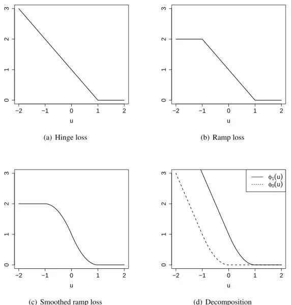
It is called the smoothed ramp loss in this work. Figure 3.2 shows the hinge loss, ramp loss and smoothed ramp loss functions. The hinge loss is the loss function used in support vector machines (Vapnik 1998). The ramp loss (Collobert et al. 2006) is also called the truncated hinge loss function (Wu and Liu 2007). It is well known that by truncating the unbounded hinge loss, ramp loss related methods are shown to be robust to outliers in the training data for the classification problem (Wu and Liu 2007). Compared with the ramp loss, the smoothed ramp loss is smooth everywhere. Hence it has computational advantages in optimization. Moreover, the smoothed ramp loss, which resembles the ramp loss, is robust to outliers too. In the framework of RWL, subjects who did not receive optimal treatment assignments but had large positive residuals, or those who did receive optimal assignments but had large negative residuals may be considered as outliers. The robustness to outliers for the smoothed ramp loss is helpful in dealing with outliers in the setting of optimal treatment regimes, especially when residuals are poorly estimated, or when the outcomeRhas a large variance.

We incorporate RWL into the regularization framework, and aim to minimize 1

n n X

i=1

b ri π(ai,xi)

T(aif(xi)) + λ 2||f||

2

(48)

−2 −1 0 1 2

0

1

2

3

u

(a) Hinge loss

−2 −1 0 1 2

0

1

2

3

u

(b) Ramp loss

−2 −1 0 1 2

0

1

2

3

u

(c) Smoothed ramp loss

−2 −1 0 1 2

0

1

2

3

u

φ1(u) φ0(u)

(d) Decomposition

Figure 3.2:Hinge loss (a), ramp loss (b), and smoothed ramp loss (c) functions. (d) shows the difference of convex decomposition of the smoothed ramp loss,T(u) = φ1(u)−φ0(u).

where||f||is some norm forf, andλis a tuning parameter. Recall that_briis the estimated residual. The smoothed ramp loss function T(u) is symmetric about the point (0,1) as shown in Figure 3.2(c). A nice property that comes from the symmetry is that the rule that minimizes the outcomeR(i.e. maximizes−R) is just opposite to the rule that maximizes R. This is intuitively sensible. However, OWL does not possess this property.

(49)

case of nonlinear learning through kernel mapping in Section 3.2.3.

Linear Decision Rule for Optimal ITR

Suppose that the decision function f(x) that minimizes (3.9) is a linear function of x, i.e. f(x) = wTx +b. Then the associated ITR will assign a subject with clinical covariatesxinto treatment 1 ifwTx+b > 0and−1otherwise. In (3.9), we define||f|| as the Euclidean norm ofw. Then minimizing (3.9) can be rewritten as

min

w,b λ 2w

T_w₊ 1 n

n X

i=1

b ri π(ai,xi)

T ai(wTxi+b)

. (3.10)

The smoothed ramp loss is a non-convex loss, and as a result, the optimization problem in (3.10) involves non-convex minimization. This optimization problem is difficult since there are many local minima or stationary points. For instance, any(w, b) with w = 0

and |b| ≥ 1 is a stationary point. Similar with the robust truncated hinge loss support vector machine (Wu and Liu 2007), we apply the d.c. (Difference of Convex) algorithm (An and Tao 1997) to solve this non-convex minimization problem. The d.c. algorithm is also known as the Concave-Convex Procedure (CCCP) in the machine learning community (Yuille and Rangarajan 2003). Assume that an objective function can be rewritten as the sum of a convex partQvex(Θ)and a concave part Qcav(Θ). The d.c. algorithm as shown in Algorithm 1 solves the non-convex optimization problem by minimizing a sequence of convex subproblems. One can easily see that the d.c. algorithm is a special case of the Majorize-Minimization (MM) algorithm.

Algorithm 1:The d.c. algorithm for minimizingQ(Θ) =Qvex(Θ) +Qcav(Θ). InitializeΘ(0)

repeat

Θ(t+1) ₌_argmin

(50)

Let

φs(u) =           

0 ifu≥s

(s−u)2 _if_s₋₁_≤_{u < s} 2s−2u−1 ifu < s−1

.

Note that φs is smooth. We have a difference-of-convex decomposition of the smoothed ramp loss,

T(u) =φ1(u)−φ0(u), (3.11)

as shown in Figure 3.2(d). DenoteΘas(w, b). Applying (3.11), the objective function in (3.10) can be decomposed as

Qs(Θ) = λ 2w

T_w₊ 1 n

n X

i=1

h

φ1(ui)I(bri >0) +φ0(ui)I(bri <0) i |

b ri| π(ai,xi)

| {z }

Qvex(Θ)

−1 n n X i=1 h

φ1(ui)I(rib <0) +φ0(ui)I(rib >0) i |

b ri| π(ai,xi)

| {z }

Qcav(Θ)

,

whereui =ai(wTxi+b). For simplicity, we introduce the notation, βi =

∂Qcav ∂ui =−

1 n

hdφ₁(ui)

dui I(bri <0) +

dφ0(ui)

dui I(bri >0) i |

b ri| π(ai,xi)

, (3.12)

fori = 1,· · · , n. Thus the convex subproblem at the (t+ 1)’th iteration of the d.c. algo-rithm is

min

w,b λ 2w

T_w₊1 n

n X

i=1

h

φ1(ui)I(bri >0)+φ0(ui)I(bri <0) i |

b ri| π(ai,xi)

+ n X

i=1

β_i(t)ui. (3.13) There are many efficient methods available for solving smooth unconstrained optimization problems. In this work, we use the limited-memory Broyden-Fletcher-Goldfarb-Shanno (L-BFGS) algorithm (Nocedal 1980). L-BFGS is a quasi-Newton method that approxi-mates the Broyden-Fletcher-Goldfarb-Shanno (BFGS) algorithm using a limited amount of computer memory. For more information on the quasi-Newton method and L-BFGS, see Nocedal and Wright (2006).

(51)

Algorithm 2:The d.c. algorithm for linear RWL with the smoothed ramp loss Setto a small quantity, say,10−8

Initializeβ_i(0) = 2|bri|

nπ(ai,xi)I(rbi <0)

repeat

• Compute(wb,bb)by solving (3.13), • Updateui =ai(wb

T_x i+bb) • Updateβ_i(t+1) by (3.12) until||β(t+1)₋_β(t)_||

∞ <

Nonlinear Decision rule for Optimal ITR

For a nonlinear decision rule, the decision function f(x) is represented by h(x) +b with h(x) ∈ HK and b ∈ R, where HK is a reproducing kernel Hilbert space (RKHS) associated with a Mercer kernel function K. The kernel function K(·,·) is a positive definite function mapping from X × X to _R. The norm in H_K, denoted by || · ||_K, is induced by the following inner product:

< f, g >K= n X i=1 m X j=1

αiβjK(xi,xj),

forf(·) = Pn_i₌₁αiK(·,xi)andg(·) = Pm_j₌₁βjK(·,xj). Then minimizing (3.9) can be rewritten as

min h,b

λ 2||h||

2 K + 1 n n X i=1 b ri π(ai,xi)

Tai h(xi) +b

. (3.14)

Due to the representer theorem (Kimeldorf and Wahba 1971), the nonlinear problem can be reduced to finding finite-dimensional coefficients vi, and h(x) can be represented as Pn

j=1vjK(x,xj). Thus the problem (3.14) is transformed to min v,b λ 2 n X i,j=1

vivjK(xi,xj) + 1 n n X i=1 b ri π(ai,xi)

Tai n X

j=1

vjK(xi,xj) +b

(52)

Following a similar derivation to that used in the previous section, the convex subproblem at the(t+ 1)’th iteration of the d.c. algorithm is as follows,

min

v,b

λ 2

n X

i,j=1

vivjK(xi,xj)

+1 n

n X

i=1

h

φ1(ui)I(bri >0) +φ0(ui)I(rbi <0) i |

b ri| π(ai,xi)

+ n X

i=1

β_i(t)ui,

where ui = ai Pn_j₌₁vjK(xi,xj) +b

. After solving the subproblem by L-BFGS, we update β(t+1) _{by (3.12). The procedure is repeated until} _β _{converges. When we obtain}

the solution(v_b,bb), the decision function isfb(x) =Pn_j₌₁ b

vjK(x,xj) +bb. Note that if we choose a linear kernelK(x,z) = xTz, the obtained rule reduces to the previous linear rule. The most widely used nonlinear kernel in practice is the Gaussian Radial Basis Function (RBF) kernel, that is,

Kσ(x,z) = exp−σ2||x−z||2,

whereσ > 0is a free parameter whose inverse1/σis called the width ofKσ.

3.2.4 A general framework for Residual Weighted Learning

We have proposed a method to identify the optimal ITR for continuous outcomes. How-ever, in clinical practice, the endpoint outcome could also be binary, count, or rate. In this section, we provide a general framework to deal with all these types of outcomes.

The procedure is described as follows. First, estimate the conditional expected out-comes given clinical covariates X, Eb

R

2π(A,X)

X

(53)

continu-ous outcomes,ri_b = ri −Eb

R

2π(A,X)

X =x_i

; if smaller values ofR are preferred,e.g. the number of adverse events, then _bri = Eb

R

2π(A,X)

X =x_i

−ri. Third, identify the decision functionfb(x)by using the estimated

b

ri in RWL.

The underlying idea is simple. Generally, the outcomeRis a random variable depend-ing on X and A. We estimate common effects of X by ignoring the treatment assign-ment A, and then all information on the heterogeneous treatment effects is contained in the residuals. As demonstrated previously, the benefits from using residuals include sta-bilizing the variance and controlling the treatment matching factor, both of which have a positive impact on finite sample performance. In previous sections, we discussed RWL for continuous outcomes in detail. We will provide two additional examples to illustrate the general framework.

The first example is for binary outcomes, i.e. R ∈ {0,1}. Assume that R = 1 is desirable. We may fit a weighted main effects logistic regression model,

E(R|X) = exp(β0+X T_β) 1 + exp(β0+XTβ)

.

The estimatesβb₀ andβbcan be obtained numerically by statistical software, for example, the glm function in R. The residual_briisri− exp(βb0+XTβb)

1+exp(βb0+XTβb)

. Then we estimate the optimal ITR by RWL.

The second is for count/rate outcomes. We use the pulmonary exacerbation (PE) out-come of the cystic fibrosis data in Section 3.6 as an example. The outout-come is the num-ber of PEs during the study, and it is a rate variable. The observed data are Dn = {xi, ai, ri, ti}n

i=1, where ri is the number of PEs in the duration ti. We treat the count

ri as the outcome, and (xi, ti)as clinical covariates. We may fit a weighted main effects Poisson regression model,