Capturing atomic interactions with a graphical framework in computational protein design

(1)

Capturing Atomic Interactions with a Graphical

Framework in Computational Protein Design

by

Andrew Leaver-Fay

A dissertation submitted to the faculty of the University of North Carolina at Chapel Hill in partial fulfillment of the requirements for the degree of Doctor of Philosophy in the Department of Computer Science.

Chapel Hill 2006

Approved by:

Jack Snoeyink

Fred Brooks

Brian Kuhlman

Jan Prins

(2)

(3)

c

2006

(4)

(5)

ABSTRACT

ANDREW LEAVER-FAY: Capturing Atomic Interactions with a Graphical Framework in Computational Protein Design.

(Under the direction of Jack Snoeyink)

A protein’s amino acid sequence determines both its chemical and its physical struc-tures, and together these two structures determine its function. Protein designers seek new amino acid sequences with chemical and physical structures capable of perform-ing some function. The vast size of sequence space frustrates efforts to find useful sequences.

Protein designers model proteins on computers and search through amino acid se-quence space computationally. They represent the three-dimensional structures for the sequences they examine, specifying the location of each atom, and evaluate the stabil-ity of these structures. Good structures are tightly packed but are free of collisions. Designers seek a sequence with a stable structure that meets the geometric and chem-ical requirements to function as desired; they frame their search as an optimization problem.

(6)

(7)

ACKNOWLEDGMENTS

I would like to thank my adviser, Jack Snoeyink, for his enthusiasm for computer science and learning, his support of my research, and his patience with my missteps. His keen intellect and academic curiosity inspired me to try harder and dig deeper when approaching the many challenges open in computational structural biology. He continues to inspire me as he straddles two disciplines, both structural biology and computational geometry, while maintaining a mastery of both. If I could have as many good ideas as Jack does, then I would have graduated a lot sooner. If I did not have Jack as an adviser, I would have graduated a lot later. Jack has greatly improved my writing, keeping the bar held high, and providing rapid and copious comments on the documents I have handed him.

I would like to thank my collaborator in Biochemistry and committee member, Brian Kuhlman, for his interest in my work, for the time spent meeting with me and answering questions, for allowing me access to Rosetta and granting me permission to modify it, and for his patience – especially when I would break his code. Brian is a giant in the field of protein design, and an inspiration. You can ask him a question that takes five minutes to state, he’ll think for a few seconds, and give an illuminating one sentence answer. It has been a pleasure working with him, and I look forward to beginning a post-doc under his guidance in the coming weeks.

(8)

his encouragement and enthusiasm, and, outside of his committee responsibilities, for his help in learning about compilers.

I would like to thank Jane and Dave Richardson from Duke University for their encouragement, interest and support in working with their program, REDUCE. They are wonderful teachers and wonderful people, and I am grateful for the opportunity to work with them. I would also like to thank Michael Word from GlaxoSmithKline, and Ian Davis and Bryan Arendall from Duke for their input and help in incorporating dynamic programming into Reduce and testing that the new version behaves as it should.

I would like to thank Hans Bodlaender from the University of Utrecht for his help in computing the treewidth of many protein design interaction graphs and for his pleasant company in Mallorca. Unfortunately he could not give me any good stories about my advisor from when they worked together at the University of Utrecht, except that Jack had taught him how to make tacos. I am sure Jack would like to thank Hans too.

I would like to thank David Baker from the University of Washington for his enthu-siasm for the rotamer trie and the interaction graph and for his subtle prods to wrap up half-finished projects, usually in the form of an email sent to sixty people announcing that I will complete them shortly.

I would like to thank Loren Looger for his help in comparing dead-end elimination to dynamic programming and for the many fruitful conversations on protein design, rotamer library size, and combinatorial optimization.

I would like to thank the BioGeometry group from UNC, Duke, Stanford, and NC-A&T for providing a forum for the computational and geometric aspects of structural biology. I benefited greatly from the enthusiastic leadership of Patrice Koehl, Leonidas Guibas, Michael Levitt, Jean-Claude Latombe, Herbert Edelsbrunner, Pankaj Agarwal, and my advisor, Jack Snoeyink.

(9)

O’Brien, Deepak Bandyopadhyay, Andrea Mantler, Jun “Luke” Huan, Vince Scheib, Deanne Sammond, Kristin Dang, Xiaozhen “Jenny” Hu, Glenn Butterfoss, Xavier Am-broggio, Doug Renfrew, Yi Liu, and Suja Thomas. Their company and conversation have meant so much to me over the years.

I would like to thank the staff in the computer science department, especially Janet Jones, Karen Thigpen, Mike Stone (who helped me replace every component on my laptop except for the CD drive, the hard drive, and the keyboard), Alan Forest, Fred Jordan, Mike Carter, Tammy Pike and Sandra Neely.

(10)

(11)

List of Figures

2.1 Snap-Lock Beads . . . 10

2.2 A Short Protein . . . 11

2.3 The Twenty Amino Acids . . . 12

2.4 Dihedral Angles In Proteins . . . 15

2.5 Protein Folding Free Energy Diagram . . . 18

2.6 Secondary Structure: Alpha Helices . . . 22

2.7 Secondary Structure: Beta Sheets . . . 23

2.8 Secondary Structure: Parallel Beta Strands . . . 23

2.9 Secondary Structure: Anti-Parallel Beta Strands . . . 24

2.10 Pairwise Surface Burial . . . 27

2.11 Pairwise Decomposable Solvation Model . . . 29

2.12 Orientation Dependent Hydrogen Bond Energy Function . . . 31

2.13 Configuration Space . . . 33

2.14 Solvent-Accessible Surfaces . . . 34

2.15 Dot Contact Analysis in PROBE . . . 35

2.16 The Coiled-Coil Heptad Repeat . . . 42

2.17 Aggregation of a β-sheet protein . . . 46

3.1 A TIM Barrel Protein . . . 60

4.1 A Treewidth-2 Graph . . . 67

4.2 A Tree Decomposition . . . 68

4.3 Dynamic Programming on an Interaction Graph . . . 73

4.4 Dihedral Space Definitions for ADP . . . 80

4.5 Stiffness Descriptors for Input Edges . . . 83

4.6 Tables For Hyperedges Produced by ADP: CB e ={∅} . . . 84

4.7 Tables For Hyperedges Produced by ADP: CB e 6={∅} . . . 85

4.8 Tables For Hyperedges Produced by ADP: |CB e |>1 . . . 86

4.9 Interaction Graphs for Ubiquitin Relaxation and Redesign . . . 89

4.10 Speedup vs Error for ADP . . . 91

4.11 Low Degree Grid Graph with High Treewidth . . . 93

(16)

4.13 Flip State Pairs for ASN, GLN, and HIS . . . 97

4.14 Sole Treewidth-4 Interaction Graph . . . 104

4.15 Spatial Reach for Side-Chain Placement . . . 107

5.1 Previous Two-body Energy Table . . . 116

5.2 A Flexible Ligand . . . 119

5.3 Interaction Graph Class Diagram . . . 131

6.1 Two Example Tries . . . 135

6.2 Comparing trie vs trie() and get energies() . . . 145

7.1 PROBIK: Protein Backbone Motion By Inverse Kinematics . . . 153

7.2 FlexBB Trie-vs-Trie Calculation Order . . . 158

7.3 Local Backbone Flexibility in a TIM Barrel Design . . . 163

7.4 Distribution of Energies From Fixed And Locally-Flexible Backbone De-sign . . . 163

8.1 SAS Update Algorithm . . . 172

8.2 Speedup Against a From-Scratch Algorithm . . . 177

8.3 Sequence Diagram ofSASAInteractionGraphRotamer Substitution Al-gorithm . . . 182

(17)

List of Tables

4.1 ADP Runtimes at Rotamer Relaxation . . . 90

4.2 Redesign Task Performance Comparison . . . 92

4.3 Large Interaction Graphs . . . 105

8.1 Running Times For SASA-Update Algorithm . . . 176

(18)

(19)

Glossary

amino group a chemical group containing a nitrogen, 9

apolar an atom or chemical group lacking either a

formal or a partial charge, 18

carbonyl group a chemical group with an oxygen forming a double bond to a carbon where the carbon is not also bound to a second oxygen, 10

DEE dead end elimination, a combinatorial op-timization technique similar to branch and bound where theorems are used to prune the search space, 48

dynamic programming an efficient optimization algorithm that stores subproblem solutions which would otherwise be repeatedly computed by a recursive (expo-nential) algorithm, 62

enthalpy energy; electrostatics and gravitation both de-scribe the enthalpy of a system, 17

(20)

free energy the combination of enthalpy (energy) and en-tropy (disorder) that describes the distribu-tion of time an entity will spend in different states as well as the distribution of a popu-lation of entities between different states at a single point in time, 16

GMEC the global minimum energy conformation; in the side chain placement problem, the assign-ment of rotamers that minimizes the energy function, 38

heavy atom an atom of any element other than hydrogen; e.g. nitrogen, carbon, or oxygen, 17

hydrogen bond the energetically favorable interaction be-tween an electron-deficient hydrogen atom and an electron-rich heavy atom where the atoms’ van der Waals spheres overlap by as much as 0.4 ˚A, 17

hydrophilic “water loving,” dissolving well in water, 17 hydrophobic “water fearing,” dissolving poorly in water,

oily, 17

hydrophobic effect the driving force stabilizing protein structures wherein hydrophobic atoms are sequestered from water in protein cores, 18

hydroxyl group a chemical group of the form XOH where X is bound to neither nitrogen nor another oxygen; also called an alcohol, 30

isomer compounds or chemical groups with the same

(21)

organic acid a.k.a.a carboxyl group. a chemical group with one carbon chemically bound to two oxygen atoms and to one other atom where the carbon forms a double bond to one of the two oxygen atoms, 9

protein backbone the atoms that form the linear tip-to-tip path along the protein, as well as the carbonyl oxy-gen; the chemical backbone structure stays constant under amino-acid substitution (mu-tation) as the backbone atoms are shared by all twenty naturally-occurring amino acids,10 protein side chains the chemical groups bound to the backbone

Cα atom of each residue, 10

residue a position in a sequence of amino acids where the position’s amino-acid identity is not nec-essarily known. E.g.in design, the identity of residue 54 could be any one of the 20 amino acids, 10

rotamer rotational isomer, a conformation for an amino acid side chain described in terms of torsional (dihedral) parameters only; the other compo-nents of internal geometry – bond lengths and bond angles – are fixed, often to their ideal values, 15

(22)

(23)

Chapter 1 Introduction

Nature controls the processes of life with molecular machines calledproteins. She com-municates cell events with signal proteins, she catalyzes chemical reactions with protein enzymes, she propels organisms with muscle proteins, she even controls protein synthe-sis with other regulator proteins. Proteins represent the most efficient motors man has ever seen; the proton pump in mitochondria operates with near Carnot efficiency.

Scientists want to create new protein behavior. They want to alter existing pro-tein/protein interactions to perturb and thereby understand biochemical pathways within cells. They want to create their own machines – machines to catalyze reac-tions or bind small molecules – so that they can perform tasks for which Nature has not given them tools.

Although protein design has many practical ends, it does not take its worth only from the support it lends other scientific disciplines: it is itself a worthy scientific en-deavor. Protein design offers a unique way of testing theoretical models for protein energetics. Design insists the designer gather all of what is understood about protein structure, all structural preferences and energy models, and integrate that understand-ing to make hypotheses. The designer then asserts positive hypotheses of the form “protein X will have behavior Y.” These hypotheses can be validated by synthesizing protein X and measuring behavior Y. The results of that synthesis and measurement then add to the body of knowledge surrounding structural biology. Protein design thus advances understanding of protein energetics and protein structure.

(24)

They rely on stochastic optimization techniques as well as some exact techniques to perform their optimizations. Computer scientists have made and can make worthy con-tributions to protein design by advancing the understanding of design’s combinatorial optimization problem, and by creating useful optimization algorithms.

In addition to contributing to optimization, a computer scientist can make worthy contributions by improving the computation and representation of the energy models that designers rely upon. Designers are currently hindered from incorporating certain kinds of energy models, either from their computational expenses or their representa-tional challenges. Representation has also proven a significant hurdle in attempts to solve optimization variations that sample larger regions of protein conformation space. In this dissertation, I detail several instances where good computer science assists protein design.

1.1 Thesis Statement

The interaction graph is an expressive model for the side-chain-placement problem, pro-viding deeper insight into the problem’s complexity than previous models, and allowing extensions that model local backbone flexibility and non-pairwise decomposable energy functions, thereby improving the designs produced by protein design software.

1.2 Main Results

In this dissertation, I define the side-chain-placement problem, the interaction graph model for this problem, and demonstrate the interaction graph’s expressiveness by showing it is a better model for the problem than the model used to prove it is NP-Complete. I do this by proving the connection between the problem’s complexity and a graph property calledtreewidth. This connection cannot be proven without a graphical formulation of the problem. The connection’s proof is constructive and takes the form of a dynamic programming algorithm defined in terms of operations on an interaction graph. In addition to standard dynamic programming, I also present a modification to dynamic programming that runs faster and uses less memory by introducing controlled amounts of error into the energy function.

(25)

interactions between pairs of residues. The amount of memory an edge requires depends on properties of the vertices the edge is incident upon. The amount of memory required for the whole graph is the sum of the memory required by the vertices and edges.

Replacing the previous data structure for the representation of energies with an in-teraction graph in the design modeule of the Rosetta molecular modelling program (Si-mons et al., 1999b; Si(Si-mons et al., 1999a; Kuhlman and Baker, 2000), improves Rosetta. The interaction graph replaces a monolithic data structure that was difficult to allocate and difficult to work with. Breaking down this monolithic structure reduces memory usage for rotamer-pair energies in Rosetta by 12%. Moreover, in replacing the previous data structure, I uncovered and fixed a bug in the storage of some rotamer-pair ener-gies. Some pair energies were mistakenly left out as a direct result of the difficulty of that data structure.

The interaction graph offers a guiding principle for how new kinds of interaction energies should be stored. The graph allows extensions to cover variations on the side-chain-placement problem. In particular, I show how an interaction graph accommodates local backbone flexibility, and how an interaction graph can be used to represent non-pairwise decomposable energetics.

I present a rapid algorithm for the computation of interaction energies used for side-chain placement. This algorithm has sped the slowest step in the Rosetta’s fixed-backbone side-chain-placement subroutine by a factor of 3.5. This algorithm also allows rapid computation of the interaction energies needed when designing with local back-bone flexibility.

I demonstrate theextensibilityof the interaction graph framework by extending the graph in two ways. First, I present an interaction graph for the incorporation of local backbone flexibility into the design process. This interaction graph efficiently stores the energies needed. I present the graph to store these energies, the algorithm to compute them, and a simulated annealing algorithm to optimize both side chain and backbone conformation. Local backbone flexibility yeilds an improvement – structures designed with local backbone flexibility have a lower energy than than those designed with a fixed backbone.

(26)

amount of computation required to maintain the two surfaces. The speed is a result of the tremendous amount of data caching, made easy by the intuitive nature of the interaction graph.

This non-pairwise decomposable model yeilds an improvement – it improves reca-pitulation of native sequences in whole protein redesign and in protein/protein interface redesign, and produces structures that are more like native proteins than those struc-tures produced in the function’s absence.

1.3 Organization

• Chapter 2 introduces the elements of protein structure and of protein energet-ics. It introduces the side-chain-placement problem and reviews the literature in protein design. Finally, it describes and compares the computational techniques that structural biologists have brought to bear on the problem.

• Chapter 3 outlines the three challenges faced in protein design, tying together the literature on successful and less-than-successful protein designs. These chal-lenges are: the difficulty in finding a perfect fit for side chains into the core of a protein, which necessitates backbone conformational sampling; the difficulty of including non-pairwise decomposable energy functions into design software; and the difficulty inherent in the side-chain-placement problem. After outlining these three challenges, the chapter relates the work in this thesis toward overcoming these challenges.

(27)

ex-pense of introducing controlled amounts of error. This chapter concludes with a description of a similar problem to the side-chain-placement problem, the hydro-gen placement problem. Dynamic programming on an interaction graph solves this problem efficiently. I have incorporated the dynamic programming algorithm into an existing piece of software for hydrogen placement, REDUCE, originally written by Michael Word in Dave and Jane Richardon’s laboratory at Duke (Word et al., 1999b). The new version of REDUCE is now being distributed.

• Chapter 5 describes the how the interaction graph can serve as a data structure. The interaction graph has been part of Rosetta and in use for nearly a year. This chapter describes the previous data structure in Rosetta that stored rotamer-pair energies before the interaction graph replaced it; this data structure, though difficult to work with, was both efficient in amount of memory it used and efficient in its speed of energy retrieval during simulated annealing. The interaction graph, reduces memory use by _∼12%, and achieves the same speed during simulated annealing. This chapter also describes the class hierarchy for the object-oriented framework added to Rosetta.

• Chapter 6 presents a fast algorithm for rotamer-pair-energy computation that serves both locally-flexible-backbone side-chain placement, and fixed-backbone side-chain placement. This algorithm is now part of Rosetta, where it has been in use for fixed-backbone side-chain placement for over a year, speeding both protein design (3.5× faster) and protein folding (2× faster).

• Chapter 7 describes the incorporation of local backbone flexibility into the side-chain-placement problem. There are three aspects of this system described: the calculation of the energies needed when the backbone moves, the storage of those energies in an interaction graph, and the optimization of backbone and rotamer placement in simulated annealing. First, a simple extension to the fast rotamer-pair-energy computation algorithm from Chapter 6 efficiently computes the ener-gies needed in flexible-backbone design. Second, an extension to the interaction graph framework stores those energies. Third, a new version of simulated anneal-ing interfaces the interaction graph to perform new kinds of rotamer substitutions not used by simulated annealing in fixed-backbone design.

(28)

of burial from solvent cannot be decomposed into the sum of pair interactions. Any energy function that depends upon surface area will be non-pairwise decom-posable. I describe how to integrate surface area computations into design using an interaction graph. Optimizing the surface-area-based energy function inside side-chain placement produces designs with a better surface-area-based energy.

• Chapter 9, concludes the thesis, discusses limitations, and notes several interesting directions for future work.

1.4 Assumed Background

This thesis describes protein chemical structure and protein physical structure in sig-nificant detail. It describes in sigsig-nificant detail protein energetics and protein stability and the approaches biophysicists have taken in modeling energies and stabilities. It ex-plains the theory behind the dynamic programming algorithm presented in Chapter 4 by delving into an area of graph theory: this thesis defines the concepts oftreewith and tree decompositions as well as partial k-trees before using these definitions to analyze the behavior of dynamic programming.

The reader should have a firm understanding of complexity analysis; of NP-Com-pleteness and of Big-O notation. The reader should be aware generally of techniques for combinatorial optimization; the thesis describes in detail dynamic programming and a stochastic technique called simulated annealing, but does not describe branch-and-bound or integer linear programming, for instance. The thesis provides citations to relevant publications in protein design where these alternative optimization techniques are used, and the curious reader is encouraged to follow these citations. The reader should also have a general sense for graph theory; the thesis contains definitions for the parts of graph theory that are somewhat obscure (e.g. ak-tree), but does not contain definitions for the parts of graph theory that are common (e.g. a k-clique). I would recommendPearls in Graph Theoryby Hartsfield and Ringel (1990) for the reader that is unfamiliar with graph theory as well as the reader who wants to better learn graph theory.

(29)

reading and drawing chemical structures can be found athttp://www.chemguide.co. uk/basicorg/conventions/draw.html. There are several pieces of chemical nomen-clature the reader should know: for example, an oxygen that forms a double bond with a carbon is a carbonyl oxygen, an oxygen that forms a single bond with a carbon and a single bond with a hydrogen is ahydroxyl oxygen. The reader may find the glossary helpful in refreshing the chemical jargon contained in this thesis. In addition a useful tutorial on organic nomenclature can be found at http://chemistry.boisestate. edu/rbanks/organic/nomenclature/orgaincnomenclature1.htm.

The thesis also presumes that the reader has previously encountered the ideas of en-ergyandfree energy, specificallyGibb’s free energy. The thesis describes the concepts of enthalpyandentropy, but at a level appropriate for a review and not as an introduction to these concepts. The reader wishing to know more about free energy should consult a textbook for any introductory undergraduate course in chemistry (either organic or inorganic chemistry). Organic Chemistryby Maitland Jones (1998) is a good text.

Finally, this thesis presumes that the reader has encountered electron orbital hy-bridization theory and can easily distinguish the geometry of sp2 _{hybridized orbitals}

and sp3 _{hybridized orbitals. Again, Maitland Jones’ textbook would be a good place}

(30)

(31)

Chapter 2 Protein Structure and the

Side-Chain-Placement Problem

Structural biochemists have discovered a host of problems to pique the interest of any computer scientist. A high-level formulation of these problems that abstracts away the biochemistry can be understood by anyone with a basic knowledge of algorithms. At one level, a computer scientist can contribute to structural biochemistry by solving problems that the structural biochemists present. On a deeper level, a computer scientist that understands the biochemistry can unearth and solve new questions – possibly ones that the biochemists had initially wanted to ask but held back because there seemed no plausible solution. This thesis describes a combination of these two contributions; places where good algorithms have improved the speed or accuracy of the software biologists initially built, and places where an understanding of the underlying biochemistry has lead to the formulation of new problems. In order to provide a fuller understanding of the contributions, I begin with a detailed description of structural biochemistry.

2.1 Protein Chemical Structure

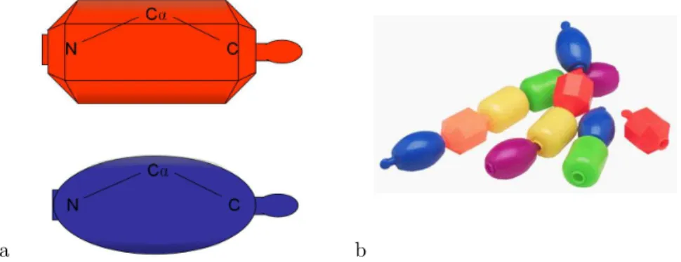
Chemically, proteins are composed ofamino acids; the tail of one amino acid is linked to the head of the next amino acid to create a one dimensional chain, much like the Snap-Lock beads of my youth (Figure 2.1a). Different amino acids link to form proteins just as snap-lock beads link to form colorful chains with interesting shapes (Figure 2.1b).

Amino acids are made up of three parts: an amino group (NH+₃), an organic acid (C(=O)O−_{) and a side chain. All amino acids share the amino and acid groups; amino}

(32)

a b

Figure 2.1: Snap-Lock Beads. a) Each snap-lock bead has a hole at one end (left) and a knob on the other (right). b) Chains of snap-lock beads are formed by connecting knobs and holes. Photo from Amazon.com

amino acids.

Amino acids are chemically linked head-to-tail to form chains. The chemical reaction that binds two amino acids together links the carbon from the acid of one amino acid to the nitrogen of the next amino acid. One of the two oxygens from the acid is converted into water and released as a product of the reaction. The chemical bond between the carbonyl carbon and the amide nitrogen is called apeptide bond. The stringing together of amino acids forms a repeating triad: -N-C-C-. From one tip of a protein to the other, there is a path that follows this N-C-C repeat. For this reason, these three atoms that make up the tip-to-tip path are often referred to as the backbone of the protein. The carbonyl oxygen is often included as a member of the backbone, though, it does not lie on the tip-to-tip path. The ambiguity over whether the carbonyl oxygen belongs in the backbone depends on which definition is meant by the word “backbone:” it could refer to the tip-to-tip path along the protein, or it can refer to everything that is not part of the side chain. In the rest of the document, I use “backbone” to mean all non-side-chain atoms.

The side chains attach to the first carbon in the N-C-C repeat. This carbon is one chemical bond away from the carbonyl carbon so it is said to be α to the carbonyl group. It is therefore called Cα. The rest of the atoms branching from Cαare similarly named with increasing Greek letters. The carbon chemically bound to Cα is called Cβ

(33)

Figure 2.2: A Short Protein. Three amino acids, methionine, serine and serine again, form this short protein. The one dimensional sequence for this protein is MSS. Note that the first residue has an NH2 group, making it the N-terminus, while the last

residue has an acid group, making it the C-terminus. These figures are skeletal formu-las; for a review of skeletal formulas, see http://www.chemguide.co.uk/basicorg/ conventions/draw.html

The sequential list of the amino acids that compose a protein captures completely the protein’s chemical structure. The convention is to list the amino acids starting from the N- (or amino-) terminus and going to the C- (or carboxy-) terminus. Each position in a protein’s sequence is referred to as a residue. It is more proper to talk about the fifty-fourth residue of a protein than to talk about the fifty-fourth amino acid. In Figure 2.2 for example, the N-terminus is residue one and is a methionine amino acid. The residue it is bound to is residue two and is a serine amino acid. The one-dimensional sequence of the amino acids is called theprimary structure. A protein’s chemical struc-ture capstruc-tures only a small part of its three-dimensional strucstruc-ture. Biologists consider four levels of protein structure. The three levels I have not yet described all pertain to three-dimensional structure.

2.2 Protein Stability

(34)

Figure 2.3: The twenty amino acids found in nature. Amino acids are often referred to by three letter or one letter codes. From left to right, with both three letter and one letter codes:

(35)

structure can be viewed as providing the structure that holds these residues in just the right relative position and orientation. Biochemists wishing to fully understand protein function must understand protein structure. A central, open problem in computational structural biology is to predict a protein’s fold given its sequence. This is called the protein folding problem.

Biochemists are able to indirectly observe protein structure. In a multi-step process called X-ray crystallography, biochemists 1) form protein crystals, 2) diffract X-rays off of the crystals and obtain the amplitudes of the diffracted X-rays, 3) transform diffraction data into electron density, and 4) thread the chemical structure through the density. In fact, the data gathered from the second stage is incomplete, and so stages three and four are often cycled between. The end product is a model containing Euclidean coordinates for the nucleus of each atom visible in the electron density. The resolution of most X-ray-determined structures is on the order of 2 ˚A. The highest resolution structures have a resolution of 0.7 ˚A.

In another multi-step process callednuclear magnetic resonance (NMR) spectrosco-py, biochemists 1) measure distances between all protein hydrogen atoms, 2) assign all the distances to specific atoms, and 3) compute a set of protein structures that satisfy the distance constraints. The resolution of NMR-determined structures is on the order of 4 ˚A. Both techniques require considerable labor and time. Nonetheless, biochemists are willing to invest time and energy in both techniques. Protein structure is that important.

X-ray crystallography may take six months from end to end. It can take months to synthesize enough protein. It can take months to crystallize the protein once there is enough to be crystallized. The X-ray diffraction step proceeds comparatively rapidly (once access to busy synchrotrons or other X-ray sources has been obtained), but the diffraction data (which describes the amplitudes of diffracted x-rays) can take months to transform (where the transformation process requires both amplitudes and phases). Model fitting following transformation is no small problem. Indeed, the absence of phase data from the diffraction step means that phases are unknown, biochemists can justifiably change the phases used in the first transformation to result in different electron densities. The stages 3 and 4 are iteratively combined: a fitted model is used to refine the phases and then to fit new models.

(36)

connected to particular atoms; the second step in NMR structure determination is to figure out a correspondence between the hydrogen atoms in the protein and the distances that have been measured. This assignment problem has been shown to be NP-Complete (Xu et al., 2002). Following assignment, the distances provide only a basic description of a protein’s structure. Distance geometry techniques are used to invert the incomplete distance matrix to produce a three-dimensional structure (Pardi et al., 1988; Crippen and Havel, 1988). What results is not a single structure, but an ensemble of structures all of which are consistent with the distance data. The ensemble is sometimes argued to reflect motion within the protein’s structure; the fewer the distance constraints on a region of the protein, the more models will be consistent with the data. On the other hand, it is not easy to argue that all the models consistent with the data reflect actual conformations the protein adopts.

Three sets of parameters describe the internal three-dimensional geometry of a pro-tein: bond lengths, bond angles, and bond dihedrals. Computational structural bio-chemists who model proteins often restrict their models to idealized bond geometries; that is they fix the bond lengths and bond angles. Biochemists restrict the source of conformational flexibility to bond dihedrals because the energetic penalties for stretch-ing bonds and flexstretch-ing bond angles far exceed the penalty in rotatstretch-ing dihedrals. As I discuss in detail later, the folded structure of a protein is only marginally stable; it is unreasonable to suspect that a folded protein strains bond lengths and angles at all. Restricting the conformation space available to models simplifies them without sacrific-ing their quality. The bond lengths and angles used come from empirical observations of small molecule crystal structures (Engh and Huber, 1991).

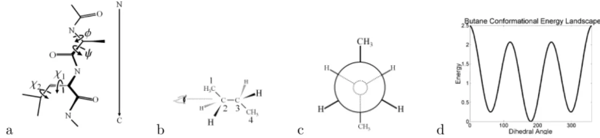
The backbone for each residue contributes two degrees of freedom from two di-hedral angles, φ and ψ (Figure 2.4a). The φ and ψ dihedrals are measured from Ci-Ni+1-Cαi+1-Ci+1 and from Ni-Cαi-Ci-Ni+1 where the subscripts on these atoms

de-note which residues they come from. The four atoms Cαi-Ci-Ni+1-Cαi+1 would define

a third dihedral for conformational flexibility; however, the structure of the molecular orbitals along the peptide bond keeps these four atoms planar. (The backbone carbonyl oxygen forms a double bond to the carbonyl carbon; this double bond requires both the backbone oxygen and the backbone carbonyl carbon adopt an sp2 _{hybridization state}

– in an sp2 _{hybridization an atom has three of its} _sp2 _{orbitals in the plane, and has}

its one p orbital perpendicular to the plane. Because the carbonyl carbon is sp2_{, the}

set of atoms Cαi, Ci, Oi and Ni+1 all lie in the same plane. The amide nitrogen, Ni+1,

(37)

carbonyl carbon. The nitrogen’ssp2 _{character places its} _sp2 _{orbitals in the same plane}

as the other four atoms, so that its bonded Cα, that is Cαi+1, lies in this same plane.

All together, the set of atoms Cαi, Ci, Oi, Ni+1, and Cαi+1 all lie in the plane. For

more on the geometry of electron orbitals and of orbital hybridization, consultOrganic Chemistry by Jones (1998)) Thus this third dihedral, ω, is either 0◦ _{or 180}◦_{, with 90%}

of observedω dihedrals at 180◦ _{(Branden and Tooze, 1999). Most structural biologists}

restrict their models to adopt planarω angles, eliminating ω as a degree of freedom.

a b c d

Figure 2.4: Protein Geometry. Protein structural flexibility results from rotatable backbone (φ and ψ) and side chain (χ1, χ2. . .) dihedrals (a). Side-chain rotamers can be understood through an example molecule, butane. Looking down the bond connecting 2 and carbon-3 in butane (b) creates a Newman projection (c). The dihedral angle can be measured as the angle between the two methyl groups in the Newman projection. Butane’s low energy conformations stagger the chemical groups bound to 2 and 3, staggering carbon-2’s groups relative to the groups on carbon-3. (d).

Side-chain conformations are also expressed in terms of dihedral angles, as bio-chemists also keep side-chain bond lengths and angles fixed. Leading away from the backbone, the side-chain dihedrals are enumerated as χ1, χ2. . .. The most limber side

chains, lysine and arginine, have four flexible dihedrals. Biochemists do not give side-chain dihedrals complete freedom, but instead limit the dihedrals to discrete values. Combining the chemical idea of isomers – compounds or chemical groups with the same elemental compositions that differ in their chemical structure – and the fact that side-chain conformers are superimposable by bond dihedral rotation, scientists refer to discrete side-chain conformations asrotamers, rotational isomers.

(38)

Ponder and Richards [1987] when they observed a sharpening of the distributions of

χ dihedral angles present in the newly deposited crystal structures which had higher resolutions than earlier structures. The early crystal structures were not sufficiently resolved to show dihedral value preferences, however as crystallography improved and the resolution increased, the dihedral angle preference became apparent. The general angle distribution shows clusters in three regions, at 60, 180 and -60 degrees. These values correspond to the staggered conformations for butane which lie at the bottom of shallow energy wells (Figure 2.4d). Ponder and Richards reported dihedral values at the bottom of these observed shallow energy wells and estimates of the ranges of these wells.

Current rotamer libraries derive from high-resolution crystal structures (Dunbrack and Karplus, 1993; Dunbrack and Cohen, 1997; Bower et al., 1997; Lovell et al., 2000; Dunbrack, 2002) and from quantum mechanical calculations (Butterfoss and Hermans, 2003). The sharpening of the dihedral angle distributions that Ponder and Richards ini-tially observed continued as crystallographic resolution improved; however, that sharp-ening has stopped. The standard deviation in dihedral angles that Lovell reported in 2000 were much smaller than the standard deviations reported by Ponder and Richards. However, the most highly resolved crystal structures do contain dihedral angles in a range surrounding the energy well bottoms and not solely at their bottoms. The pres-ence of these off-optimal dihedral values suggests that the energetic destabilization of off-optimal dihedral angles can be compensated for by improving other portions of the protein’s energy. Computational structural biochemists should therefore sample the dihedral wells at points other than their bottoms to accurately model side-chain con-formational flexibility. Indeed, protein designers have had the most success when they sample dihedral space at sub-optimal points (De Maeyer et al., 1997; Gordon and Mayo, 1998; Looger and Hellinga, 2001). As could be expected, the more rotamer samples, the more difficult the computational problems become.

(39)

en-ergy of a folded structure, one would still need to know the absolute free enen-ergy of the unfolded state in order to measure the stability of the protein. The distinction between absolute free energy of a conformation (G) and the stability of a conformation (∆G) is crucial for protein design, as designers seek the most stable structure for some purpose and not simply the structure with the lowest free energy. Biophysicists have come up with a set of energy models that can be used to compute the energy of a folded protein structure, (described in greater detail in Section 2.4); to evaluate the stability of a folded protein structure requires an idea of the protein’s energy in its unfolded state. It is insufficient to examine the interactions between protein atoms alone to determine the protein’s stability.

The free energy of a state is always a negative number, and nature prefers low free energy. This can be summed up with a variation on the old stock market saying: “buy low, sell lower.” In this dissertation, all optimizations of free energy are of minimizing free energy. The free energy of a state,Gdepends on the temperature (T), the enthalpy (H), and the entropy (S)

G=H−T ∗S.

The enthalpy of a state is what is most commonly called its energy – a distinct idea from free energy, to be sure. Gravity describes the enthalpy of two bodies: when two bodies are brought nearer together, they have a lower enthalpy. However, enthalpy is only half of free energy’s story. The entropy of the state is a function of the disorder in that state, or how many micro-states that the state ensemble consists of. The more disorder, the higher the entropy; the less disorder, the lower the entropy. The effect of entropy on the free energy of a state increases as temperature increases.

A precise understanding of the forces involved in protein stability is required to predict a protein’s fold, or to design novel proteins. While a precise understanding remains elusive, biochemists have gleaned several general rules of folded proteins. One rule is that the side chains of hydrophobic amino acids (PHE, ILE, LEU, MET, VAL, TRP) are buried from solvent in the core of a protein, while the remaining hydrophilic amino acid side chains are located towards the surface of the protein. The burial of hydrophobic amino acids, called thehydrophobic effect(Kauzman, 1959), is commonly thought to play the greatest role in stabilizing a protein’s fold. The hydrophobic effect on the molecular level stems from preferential orientation of water atoms that surround hydrophobic amino acids (Dill, 1990). This deserves explanation.

(40)

Figure 2.5: Folding coordinate diagramThe X-axis represents the “folding coordinate” where the unfolded state (U) is on the left and the folded state (F) is on the right. The Y-axis represents the absolute Gibb’s free energy of each point in the folding coordinate. The stability of a protein is the difference in free energy between its unfolded and folded states, ∆G. In protein design, the optimization problem is often one where the most stable structure is desired, as opposed to the structure with the lowest free energy. Designers must take into account the free energy of the unfolded state (which is never explicitly modeled) as well as the free energy of the folded state.

A hydrogen bond forms when any electron-rich heavy atom – where a heavy atom is any atom that is not hydrogen – shares its electrons with an electron-deficient hydrogen atom. The heavy atom to which the hydrogen is bound donates its hydrogen to the electron rich heavy atom that accepts it. The donor in a hydrogen bond is the heavy atom chemically bound to the hydrogen; the acceptor is the electron-rich heavy atom that interacts with the hydrogen.

The electron-deficient hydrogen atoms in proteins are those chemically bound to oxygen, nitrogen, or sulfur. Hydrogen atoms bound to carbon atoms cannot be donated to form hydrogen bonds. Electron-rich heavy atoms in proteins are oxygen, nitrogen, and sulfur. Carbon atoms cannot accept hydrogen bonds. The majority of the atoms in proteins are either carbon atoms or hydrogen atoms bound to carbon.

(41)

orient its hydrogen atoms toward bulk solvent. However, this orientational restriction has an entropic cost. Thus, there is a fight between entropy and enthalpy. At low temperatures, enthalpy wins and the water suffers a loss of conformational entropy: the water cannot orient itself in as many positions as it would if not next to the solute atom. At high temperatures, entropy wins and the water suffers a loss of enthalpy: the water will give in to entropy and end up pointing its hydrogen atoms at the solute atom at the energetic expense of not forming a hydrogen bond. At body temperature, enthalpy wins, and entropy loses.

Why does the hydrophobic effect stabilize a protein? The unfolded state of the protein exposes more hydrophobic surface area to water than the folded state. The more surface area a structure exposes to water, the higher the free energy of that structure. The folded state is stable because the unfolded state is at a higher energy. For example, if the free energy of the unfolded state,Gu in Figure 2.5 were to increase from where it is drawn, and the free energy of the folded state Gf were to stay the same, then the ∆G = Gf −Gu would decrease, meaning the protein would be more stable.

Entropy’s contribution toward the destabilization of the unfolded state can be ob-served through “cold-unfolding.” As temperature decreases, the effect of entropy of the free energy of the unfolded state decreases; the unfolded state is at lower free energy at lower temperatures. The decrease in the energy of the unfolded state creates a decrease in the stability of the protein; below certain temperatures, proteins unfold. At high temperatures, the protein will also unfold, however, this is due not to water, but to the low entropy of the folded state in comparison to the entropy of the unfolded state, and the greater importance of entropy at higher temperatures.

(42)

hydrogen bonding groups were in fact accessible to solvent (Fleming and Rose, 2005). “The difference between ∼90% and ∼100%,” he argues, “is the difference between a trend and a rule.” Buried hydrogen bonding groups form intra-molecular hydrogen bonds.

Folded proteins are also subject to electrostatic forces. Coulomb’s law expresses the interaction energy of two charged particlesi and j with charges qi and qj as

Eelectrostatics(i, j) =

qiqj

ǫ1dij

(2.1)

wheredij is the distance between the two, andǫ1is the dielectric constant. The function

describing Coulomb’s law has a peculiar shape. The interaction that atom i has with nearby atom j has more influence on i’s energy than the interaction it has with atom

k further away. However, because the drop off is a function of 1_d, the interactions that atomihas with all atoms at distanced1 contribute less than the interactions ihas with

all atoms at distance d2 > d1, since there are more atoms at distance d2. This can be

understood by looking at the volume of a spherical shell of radius d and thickness ∆, which is 4πd2_{∆, and the influence contributed by all atoms inside this shell (assuming}

a uniform density of ρatoms per unit volume, and that each atom j interacting withi

at this distance has a charge of qj):

4πd2∆ρǫ1

qi∗qj

d = 4π∆ρǫ1qiqjd.

The influence contributed from each shell increases with distance! In general, any energy function that drops off according to d−k _{is short ranged if} _{k >} _{3 and} long-ranged ifk <3 (Bromberg and Dill, 2003). At k = 2, all spherical shells contribute the same towardi’s energy. Atk = 3, the contribution for the shell at radiusddrops off as a function of 1_d – this drop off is slow enough that such energy functions are described as long ranged. (The sum Pn

x=1x−1 does not converge as n goes to infinity – the sum Pn

x=1x−2 on the other hand does converge.)

(43)

been left out entirely suggest long range electrostatics are unnecessary (Bradley et al., 2005). At the very least, close interactions between oppositely charged side chains, (e.g. LYS+ _{and GLN}−_{), are often observed near the surface of proteins. These interactions}

are calledsalt bridges as they resemble the close interactions of oppositely charged ions in salts.

Finally, proteins are also stabilized by London dispersion interactions, which are also called van der Waals interactions. Uncharged, freely rotating dipoles attract each other with a function proportional tod−_ij6 (for the proof, see [Bromberg and Dill, 2003]). The Lennard-Jones 6-12 potential approximates the van der Waals interactions for atomsi

and j with radii Ri and Rj by

EvdW(i, j) =ǫ(

R_i+R_j

dij

12

−Ri_d+Rj

ij

6

) (2.2)

where ǫ is the energy at the bottom of the contact well. The d−_ij6 term captures the attractive forces of dipole interactions from statistical thermodynamics; the d−_ij12 term is meant to capture the repulsive forces preventing non-bonded atoms from colliding. The principle reason the d−_ij12 term is used is its computational convenience as the square of the d−ij6 term.

2.3 Hierarchy of Protein Structure

Biochemists talk about protein structure on four levels: primary, secondary, tertiary and quaternary. Primary structure, as mentioned earlier, is the linear sequence of amino acids that compose the protein. Primary structure can be represented as a string, where each amino acid in the protein is represented by its one-letter code (Figure 2.3).

(44)

a b c

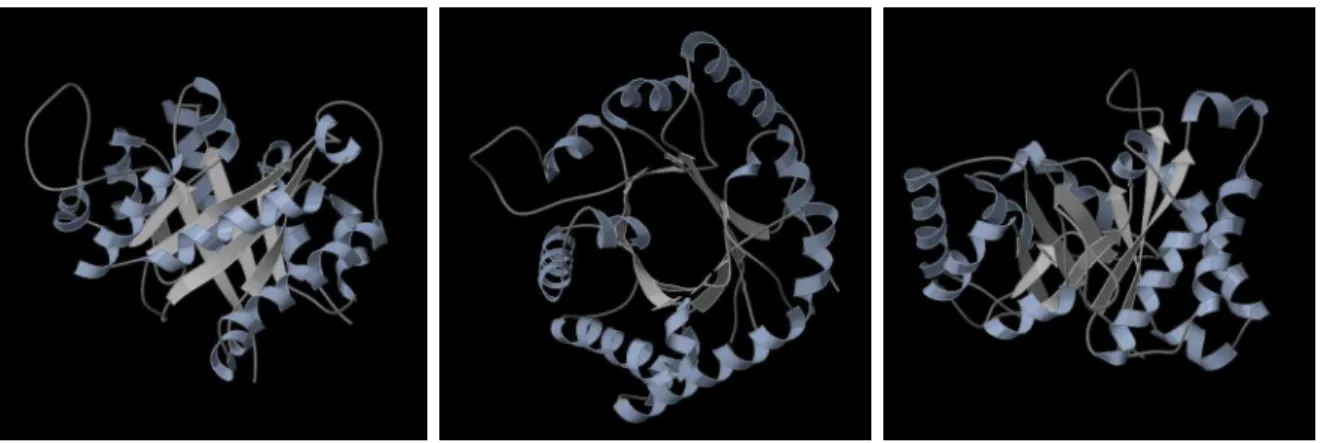
Figure 2.6: Ubiquitin’s Alpha Helix. a) Cartoon and b) ball and stick representations of the α-helix in ubiquitin. The carbonyl oxygens atoms (red) point in the direction towards the C-terminus (up). The nitrogen atoms (blue) point their bound hydrogen atoms towards the N-terminus (down). In c) the outward splaying of the carbonyl oxygens is apparent when viewed down the center of the helix.

secondary structure does not suggest much about side-chain conformation. The other part of α-helices’ and β-sheets’ low rank is simply their commonality. Helices and sheets are found everywhere; complex structures are built from various arrangements of secondary structures.

In an alpha helix (Figure 2.3), the backbone is wrapped in a tight coil. The carbonyl oxygen on residueiforms a hydrogen bond with the backbone nitrogen on residuei+ 3. The hydrogen bond betweeniandi+3 positions the carbonyl oxygen on residuei+1 so that it can form a hydrogen bond with residuei+4. The helices are almost always right-handed – as Jane Richardson would say, as you climb the spiral staircase of the helix, you use your right hand to hold the rail. Left-handed helices have been observed in protein structures, but they are very short – 4 or 5 residues. For a residue in the middle of the helix – that is, not near the ends of the helix – both the residue’s carbonyl oxygen and the nitrogen groups form hydrogen bonds with the backbone nitrogens and oxygens of other helix residues. For a residue at either end of the helix, one of its backbone hydrogen bonding groups is left to find some non-backbone hydrogen bonding partner – either water, or a side-chain hydrogen-bonding group.

(45)

a b

Figure 2.7: Ubiquitin’s Beta Sheet. a) Cartoon and b) ball and stick representations of ubiquitin’s beta sheet. The top strand and the middle strand show a parallel arrange-ment, the middle strand and the bottom strand show an anti-parallel arrangement.

(46)

Figure 2.9: Anti-Parallel Beta Strands. If two β-strands align so that their N-to-C orientations point in opposite directions, they are able to form a regular pattern of hydrogen bonds. The hydrogen atom bound to each backbone nitrogen is not shown.

Sequence analysis of secondary structures in proteins reveals that some amino acids are more likely to form α-helices than others, while others are more likely to form β -sheets (Chou and Fasman, 1978; Garnier et al., 1978; Richardson and Richardson, 1988; O’Neil and DeGrado, 1990; Munoz and Serrano, 1994). The statistics can be interpreted as natural propensities for amino acids to form helices or sheets. Biochemists have used these propensities to predict protein secondary structure and from there the complete folded structure (Cohen et al., 1982).

Tertiary structure depends significantly upon side chains. Tertiary structure is a little frustrating to define; certainly specifying the location for all atoms in the pro-tein defines its tertiary structure, however, biochemists often refer to the topological arrangement of secondary structures as tertiary structure (Richardson et al., 1992), as well as some specific types of interactions between pairs of side chains. Structural elements described as elements of tertiary structure include the protein’s fold classi-fication (Murzin et al., 1995), the hydrogen bonding pattern of β-sheets, side-chain salt bridges, the tight packing of hydrophobic side chains in protein cores and disul-fide bonds (chemical bonds formed between the sulfur atoms in cysteine side chains). Disulfide bonds constitute the exception to the rule that protein chemical structure is captured completely by its primary structure – these chemical bonds are not captured in a one-dimensional sequence.

(47)

2.4 Energy Functions

Computational biochemists must be able to evaluate the energy of a particular struc-ture. They express energy as a function of the coordinates of the protein. As bio-chemists manipulate the structure of a protein, they want to know if their manipu-lations improve (decrease) or degrade (increase) the protein’s energy. Expressing the energy of a structure is both extremely important and extremely difficult, and has been the study of biophysicists for decades.

One form of energy function comes from the field of molecular dynamics. Molecular dynamics attempts to model protein motion using numerical integration of Newtonian-like functions of protein energetics. Several “force fields” for molecular dynamics have been developed such as Amber (Weiner et al., 1986; Cornell et al., 1995) and CHARMM (Brooks et al., 1983; MacKerell et al., 1998). The shape of the functions in these force fields are consistent across all force fields: what varies are the coefficients chosen to fit the fields to experimental data. The energy of an entire system can be described by the sum of five energy terms. The first three terms, bond length stretch, bond angle flex and dihedral twist, reflect the energetics between atoms separated by very few chemical bonds. The last two terms are applied to those atoms separated by at least three chemical bonds. Specifically, these terms look like

Etotal =

P

i,j bondedEstretch(i, j) +

P

i,j,k neighboringEflex(i, j, k)

+ P

i,j,k,l neighboringEtwist(i, j, k, l)

+ P

i,j non−bondedEelectrostatics(i, j)

+ P

i,j non−bondedEvdW(i, j)

(2.3)

where the individual atoms are iterated over in each sum.

(48)

dynamics, pairwise decomposability of the energy function implies that the energy derivative for an atom can be computed analytically as the sum of the derivatives for each of its interactions.

Pairwise decomposability plays a large role in the Rosetta molecular modeling pro-gram. Rosetta contains a gradient-based minimizer that works directly in torsion space; the minimizer computes derivatives for bond dihedrals (Abe et al., 1984). These deriva-tives for dihedrals rely on the pairwise decomposability of the energy function. Torsional derivatives allow Rosetta to preserve ideal bond lengths and angles throughout protein folding trajectories, unlike molecular dynamics simulations which are also able to re-lax a structure, but require that bond angles and bond lengths be flexible. In protein design, pairwise decomposability allows the precomputation of residue pair energies so that the optimization phase need not compute any energies. Chapter 5 discusses pairwise decomposability’s role in protein design in greater detail.

2.4.1 Solvation Energy Functions

In many molecular dynamics simulations, water is explicitly modeled along with the protein. In the absence of explicit water, proteins modeled with the energy function in Equation 2.4 unfold over the course of a molecular dynamics trajectory. By including water along with the protein, one can maintain proteins’ folded states. So in addition to the thousands of atoms in a single protein, a biophysicist must include tens of thousands of water molecules (Berne, 1977). Getting the right water model has been an important topic in molecular dynamics (Jorgenson et al., 1983; Hermans et al., 1988; Silverstein et al., 1998). Modeling water explicitly costs much more than modeling a protein by itself and considerable effort has been directed at simulating only as much water as is necessary (Brooks and Karplus, 1983; Brungler et al., 1985; Brooks and Karplus, 1989). In protein design, the expense of modeling water explicitly would be prohibitive. Designers do not run molecular dynamics simulations during the course of their design calculations. To avoid the costs associated with modeling water explicitly, attempts have been made to express water’s effects implicitly.

(49)

Figure 2.10: Pairwise Surface Burial. (a) The portion of residue i that is not buried from solvent by the backbone (b) Residuej buries some ofi’s surface from water (blue dots). (c) Residuekburies some ofi’s surface from water. (d) Together, residuesjandk

bury some ofi’s surface doubly (red dots). In Street and Mayo’s pairwise decomposable energy function, this region is doubly counted, and over-counting in general is treated by scaling.

atom buries a certain portion of the surface of another atom, that surface portion cannot become more buried by the approach of a third atom. Because the solvent-accessible-surface area (SASA) is not decomposable into a sum of pairs, exact SASA-based solvation models have not been previously incorporated into the optimization step of protein design software.

(50)

Lazaridis and Karplus proposed an implicit solvation model that is decomposable into the sum of atom pair interactions (Lazaridis and Karplus, 1999). They conceived of a field, Fi, that surrounds atom i where the field describes for a point in space the solvation energy contributed by that point if it were occupied by water. An atomj that approaches i excludes water from occupying a region of space surrounding i (Figure 2.11). They define the change in the free energy of solvation of atom i, ∆Gslv

i , caused by placing a single atom j in i’s solvation field as the difference between a reference solvation energy, ∆GREF

i and a volume integral over this field: ∆Gslvi = ∆G

REF i −

Z

Vj

Fi(r)dr. (2.4)

They define the change in free energy of solvation induced by all atomsj that surround

i as

∆Gslv

i = ∆G REF i − X j Z Vj

Fi(r)dr (2.5)

Having decided upon the form of a volume integral, they needed a function F to describe the field. They observed that the first solvation sphere surrounding an atom accounted for_∼84% of the solvation energy. They also noticed that the error function, which is given by

erf(y) = √2

π

Z y 0

e−x2dx.

evaluates to 84% for erf(1). Thus to describe the field, thesolvation free energy density, for a point at a distance ofr from the center of atomi with radiusRi, with correlation distanceλi, and with a field intensity of αi they chose the following function:

Fi(r) = αie

−(r−_λRi)2

4πr2 (2.6)

(51)

(52)

αi were chosen to penalize the burial of hydrophilic groups, and reward the burial of hydrophobic groups.

Lazaridis and Karplus tested their implicit solvation model with molecular dynam-ics. As mentioned before, in molecular dynamics simulations that do not include explicit or implicit solvent, the protein molecules tend to unfold over time. The force field de-scribed in Equation 2.4 is unable to keep a protein folded in vacuo. When Lazaridis and Karplus included their implicit solvation model, the proteins they simulated did not unfold.

2.4.2 Hydrogen Bond Energy Functions

Originally, hydrogen bonding in molecular dynamics was not modeled separately from the electrostatic terms. Recent force fields include a specific hydrogen bonding term given by a 10-12 potential:

Ehb(i, j) = (

R_ij

dij

12

−Rij

dij

10

)

defined similarly to the Lennard-Jones 6-12 potential, but shorter-ranged.

Kortemme et al. introduced a knowledge-based hydrogen bonding potential that aimed to capture the geometric specificity that comes from the quantum mechanics (Ko-rtemme et al., 2003). Quantum mechanics predicts the electron orbital geometry ofsp2

hybridized atoms (such as the backbone carbonyl oxygen) to have the three sp2

or-bitals in the plane with 120◦ _{between each orbital, and to have their fourth orbital,}

a p orbital, perpendicular to that plane. Quantum mechanics also predicts that sp3

hybridized atoms (such as serine’s hydroxyl oxygen) will position their foursp3 _orbitals

in a tetrahedral geometry, with 109◦ _{between them. Since hydrogen bonding occurs}

when a hydrogen atom is positioned inside the electron density of the acceptor atom, the geometry of the electron orbitals should play a role in the energy of the hydrogen bond. The better the overlap between the hydrogen atom and the electron orbital, the stronger the hydrogen bond. However, previous hydrogen bond models effectively treated the electron orbitals as if they were spherical by not including any degree of directional sensitivity.

Kortemmeet al.’s knowledge-based function explicitly includes directional sensitiv-ity. Their function is the sum of three terms:

(53)

Figure 2.12: Orientation Dependent Hydrogen Bond Energy Function. Kortemme et al.defined a hydrogen bond function in terms of three parameters the donor/acceptor distance, the donor/acceptor/acceptor-base angle (φ), and the acceptor/donor/donor-base angle (θ). The first angle reflects the location of the electron orbitals. For example, carbonyl oxygen atoms are sp2 hybridized, with their two lone pairs in the plane of the carbon and the two atoms bound to that carbon. These orbitals are 120◦ _{away from}

the C-O bond vector. The statistics Kortemmeet al. mined from the PDB agreed with the geometric intuition from quantum mechanics. The second angle, Θ, captures the orientation of the dipole, giving a preference for hydrogen bonds where Θ is 180◦_.

where i represents the donor hydrogen and j represents the acceptor, ib is the donor-base, the heavy atom to which iis bonded, and jb is the acceptor-base, a heavy atom to which j is bound that serves to orient j (Figure 2.12). The first term in this function,

Ehb−dist(i, j) is a function of the separation distance between i and j. The next term,

Ehb−θ(i, j, ib) is a function of the angle defined by the donor-base the donor-hydrogen

and the acceptor and prefers to be at 180◦_{. The last term,} _E

hb−φ(i, j, jb) is a function

of the angle defined by the donor-hydrogen the acceptor and the acceptor-base. When the acceptor is a carboxy oxygen, this last function prefers an angle of 120◦_{. When the}

acceptor is a hydroxyl oxygen, this last function prefers an angle of 109◦_.

(54)

2.4.3 Non-Pairwise Decomposable Energy Functions

Although pairwise decomposability offers computational efficiency, several contributors to protein stability cannot be described as the sum of pair interactions. In particular, the effects of solvent, both in the way it forces hydrophobic groups to the core, and in the way it forces buried hydrophilic groups to form intra-molecular hydrogen bonds, cannot be accurately described as a sum of pairs. This is unfortunate for protein design in that solvent plays a prominent role in protein stability. Optimizing protein sequence for stability requires either approximating solvent’s effects with a pairwise decompos-able energy function or optimizing sequence using a non-pairwise decomposdecompos-able energy function.

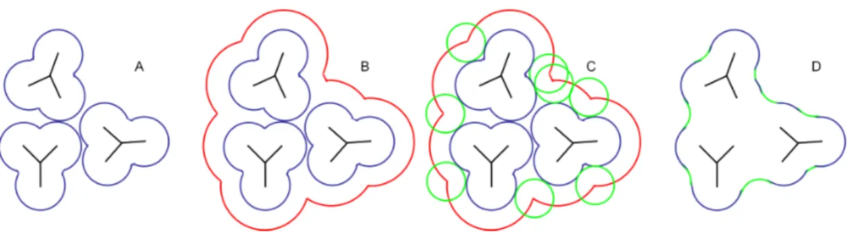
As mentioned before, the stability provided by the hydrophobic effect is proportional to the amount of buried hydrophobic surface area. The amount of buried surface area cannot be quantified without knowing the location of all atoms in the protein. Even once all of the atom locations are known, computing the SAS is still challenging. Lee and Richards defined the solvent-accessible surface as the surface produced by enlarging the van der Waals radius of the protein atoms by the radius of a water molecule, 1.4 ˚

A (Lee and Richards, 1971). This is mathematically equivalent to the Minkowski sum as defined within robotics.

Suppose a robot is asked to move through some region that contains obstacles (Figure 2.13). The robot must compute where it can fit without colliding with the obstacles. It finds the regions it can fit into by considering the accessible regions of a new space calledconfiguration space. In configuration space, the robot has been shrunk to a single point – its center, perhaps – and all of the obstacles are larger than they were in the original space. The size and shape of the obstacles in configuration space is defined mathematically by computing the Minkowski sum of the obstacles and the robot.

If both robots and obstacles are made of circles in 2D or spheres in 3D, the com-putation of configuration space is easy: the Minkowski sum produces a new set of configuration space obstacles which are themselves circles or spheres with radii that are the sum of the robot’s radius and original obstacles’ radii.

(55)

Figure 2.13: Configuration Space The Minkowski sum of a circular robot (blue) and circular obstacles (gray) produces obstacles in configuration space whose radii are the sum of the robot’s and the obstacle’s radii. A point on the surface of the union of the configuration space obstacles represents a position the center of the robot could be in Cartesian space without colliding with the obstacles. Because the configuration space obstacles overlap, the robot may not pass between them.

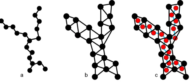
atom it originated from and the 1.4 ˚A radius of water. The surface of the union of the configuration-space spheres is the solvent-accessible surface (Figure 2.14b). Each point on the configuration space surface maps to a point in 3-D where the center of a water molecule can fit without colliding with the protein.

To compute the SAS requires computing the surface of a set of overlapping spheres. This is non-trivial. Recent techniques in computing the SAS include maintaining a spherical arrangement (Eyal and Halperin, 2005) for the enlarged spheres. With a spherical arrangement, the solvent-accessible surface can be computed exactly. Un-fortunately, the computational expense of maintaining a spherical arrangement for a moving structure is large. Shrake and Rupley proposed a numerical approximation technique for computing the SAS (Shrake and Rupley, 1973). They sampled the sur-face of each enlarged sphere with 92 dots. Each dot was the representative of a sursur-face patch. Summing the surface area for each patch whose representative dot is not con-tained inside any other enlarged sphere yielded the SASA. (They tested using up to 400 dots but decided that 92 were sufficient).