Printed in Great Britain
On inverse probability-weighted estimators in the presence
of interference
BYL. LIU
School of Statistics, University of Minnesota at Twin Cities, 224 Church St SE #313, Minneapolis, Minnesota 55455, U.S.A.
M. G. HUDGENS
Department of Biostatistics, University of North Carolina, CB #7420, Chapel Hill, North Carolina 27599, U.S.A.
ANDS. BECKER-DREPS
Department of Family Medicine, University of North Carolina, CB #7595, Chapel Hill, North Carolina 27599, U.S.A.
SUMMARY
We consider inference about the causal effect of a treatment or exposure in the presence of interference, i.e., when one individual’s treatment affects the outcome of another individual. In the observational setting where the treatment assignment mechanism is not known, inverse probability-weighted estimators have been proposed when individuals can be partitioned into groups such that there is no interference between individuals in different groups. Unfortunately this assumption, which is sometimes referred to as partial interference, may not hold, and more-over existing weighted estimators may have large variances. In this paper we consider weighted estimators that could be employed when interference is present. We first propose a generalized inverse probability-weighted estimator and two Hájek-type stabilized weighted estimators that allow any form of interference. We derive their asymptotic distributions and propose consistent variance estimators assuming partial interference. Empirical results show that one of the Hájek estimators can have substantially smaller finite-sample variance than the other estimators. The different estimators are illustrated using data on the effects of rotavirus vaccination in Nicaragua.
Some key words: Causal inference; Interference; Inverse probability-weighted estimator; Observational study.
1. INTRODUCTION
In causal inference it is often assumed that there is no interference between individuals, i.e., that the treatment of one individual does not affect the outcome of another. However, this assumption may not hold. For instance, in infectious disease studies, the vaccination status of one individual may affect whether another individual becomes infected (Halloran & Struchiner,1995). Simi-larly, encouraging one individual to vote may increase the likelihood that another individual in
the same household will vote (Nickerson,2008). Interference may also occur between students in the same classroom (Hong & Raudenbush,2006) or between households in the same neighbour-hood (Sobel,2006), and in myriad other contexts (Rosenbaum,2007;Luo et al.,2012;Manski,
2013).
Inference in the presence of interference is interesting, because a treatment may have multiple types of effects, but difficult, because individuals may have many potential outcomes. Recently, methods have been developed for the setting where individuals can be partitioned into groups such that there may be interference between individuals in the same group but not between individuals in different groups; this is sometimes called partial interference (Sobel,2006). Assuming partial interference, Hudgens & Halloran (2008) defined the direct, indirect, total and overall causal effects of a treatment in randomized studies. Inference about these types of causal effects has subsequently been considered byVanderWeele & Tchetgen Tchetgen(2011),VanderWeele et al.
(2012),Halloran & Hudgens(2012),Liu & Hudgens(2014) and P. M. Aronow and C. Samii in an unpublished 2013 paper (arXiv:1305.6156), among others. For observational settings where the treatment assignment mechanism is not known,Tchetgen Tchetgen & VanderWeele(2012) proposed inverse probability-weighted estimators of these causal effects based on group-level propensity scores. These weighted estimators can be viewed as a generalization of the usual inverse probability-weighted estimator of the causal effect of a treatment in the absence of inter-ference. However, in general, weighted estimators are known to have relatively large variance. Additionally, in some settings the partial interference assumption may be dubious. In this article we consider alternative weighted-type estimators that allow for general forms of interference and tend to be less variable.
2. PRELIMINARIES
Consider a finite population of nindividuals, and suppose that each individual may receive some treatment or exposure. LetZi (i = 1,. . .,n) be the random variable such that Zi = 1 if
individualireceived treatment andZi =0 otherwise. Suppose that interference may be present
between the n individuals, and define the interference setχi = {i1,i2,. . .} for individual ito be an ordered set of all other individuals whose treatment received might affect the outcome of individuali. Assume that there is no interference between individualiand individuals not inχi. There may or may not be interference between individualiand individuals inχi. A central goal of the inferential methods described below is to quantify the extent to which such interference is present. LetSi = (Zi1,Zi2,. . .)denote the vector of treatment indicators for individuals that
possibly interfere with individual i; that is, the outcome of individual i is allowed to depend not only onZi but also onSi. For example, if the outcome of individual 1 possibly depends on
their own treatment status as well as that of individuals 2 and 3 but not on that of individuals 4,. . .,n, thenχ1= {2, 3}andS1=(Z2,Z3). The interference setsχ1,. . .,χnare assumed to be known a priori. Denote possible values ofZiandSibyziandsi. Letyi(zi,si)denote the potential
outcome of individual iif they receive treatment zi and their interference set receives si. This
potential outcome notation is general enough to encompass any possible interference structure, of which partial interference is a special case. LetYi =yi(Zi,Si)denote the observed outcome.
The potential outcomesyi(zi,si)are assumed to be deterministic functions ofzi andsi, and the
observed outcomeYiis considered to be random because it depends on the random variablesZi
andSi. Let
Si be the sum over all the components ofSi, and let|Si|denote the dimension of
the vectorSi. For example, ifS1 =(Z2,Z3), then
S1 =Z2+Z3and|S1| =2.
in the population is treated with that of the counterfactual scenario where every individual in the population is not treated. Similarly, in the presence of interference, causal estimands can be defined in terms of counterfactual scenarios corresponding to different treatment allocation strategies (e.g., Hong & Raudenbush, 2006; Sobel, 2006;Hudgens & Halloran, 2008; Tchet-gen TchetTchet-gen & VanderWeele,2012). For example, the indirect effect, defined formally below, contrasts average outcomes of untreated individuals for the counterfactual scenario where one allocation strategy is adopted in the population with those for the counterfactual scenario where some other allocation strategy is adopted in the population. Such estimands quantify interference, if present, at the population level and can be used to inform policy decisions regarding a treatment or exposure. The allocation strategy of interest will in general depend on the setting.
Here we consider Bernoulli allocation strategies proposed byTchetgen Tchetgen & Vander-Weele(2012), where strategyα corresponds to the counterfactual scenario in which individuals independently receive treatment with probability α. It is not assumed that the observed treat-ment indicatorsZ1,. . .,Znare independent Bernoulli random variables; rather, the distribution
of treatment under Bernoulli allocation is used below to define the counterfactual estimands of interest. By analogy, direct standardization of mortality rates could entail using the 2010 United States census age distribution, which may differ from the age distribution giving rise to the observed data. Corresponding to Bernoulli allocation, letπ(si;α)=αsi(1−α)|si|−si denote
the probability of the interference set for individual i receiving treatment si under allocation
strategy α. Let π(zi;α) = αzi(1−α)1−zi and π(zi,si;α) = π(zi;α)π(si;α) denote,
respec-tively, the probability of individual i receiving treatment zi and the probability of individual
i together with their interference set receiving joint treatment(zi,si)under allocation strategy α. Define y¯i(z,α) = siyi(zi = z,si)π(si;α)to be the average potential outcome of
individ-ual i under allocation strategy α, where the summation is over all 2|Si| possible values of s
i.
Returning to the example where S1 = (Z2,Z3), the average potential outcome of individual 1 is a weighted average of potential outcomes under different combinations of treatmentZ1 = z and(Z2,Z3) ∈ {(0, 0),(0, 1),(1, 0),(1, 1)}, with the weights being the corresponding probabil-ities under Bernoulli allocation. Averaging over all individuals, define the population average potential outcome asy¯(z,α)=in=1y¯i(z,α)/n. Similarly, define the marginal average potential
outcome for individual iunder allocation strategyα by y¯i(α) = zi,siyi(zi,si)πi(zi,si;α)and
define the population marginal average potential outcome asy¯(α)=ni=1y¯i(α)/n.
Various causal effects can be defined by contrasts in the population average potential out-comes. In particular, define the direct effect of treatment under allocation strategy α to be
¯
DE(α) = g{¯y(1,α),y¯(0,α)}, whereg(·,·) is some continuous contrast function. A commonly
used contrast function isg(x1,x0)=x1−x0; in vaccine trials with a binary outcome it is typical to useg(x1,x0)=1−x1/x0. The direct effect compares the average potential outcomes when an individual receives treatment versus not under allocation strategyα. For two allocation strategies
effect, which describes the contrast in average outcomes under one allocation strategy relative to another.
3. INVERSE PROBABILITY-WEIGHTED AND HÁJEK-TYPE ESTIMATORS
In this section we propose inverse probability-weighted and Hájek-type estimators which allow for general interference; that is, no assumption is made regarding the structure or form of interference that might be present. When there is partial interference and the groups are of the same size, the inverse probability-weighted estimators defined below reduce to those proposed byTchetgen Tchetgen & VanderWeele(2012). Aronow and Samii (arXiv:1305.6156) considered similar estimators in the setting where interference may be present, but where treatment is assigned randomly according to a known experimental design.
Let li denote a vector of pretreatment covariates of individuali, and letlχi = (li1,li2,. . .).
Assume that conditional on covariates li, the treatment allocation for individuali is
indepen-dent of all potential outcomes and other covariates; that is, pr(Zi = zi | li) = pr{Zi = zi |
l1,. . .,ln,y1(·),. . .,yn(·)}. Likewise, assume pr(Zi =zi,Si =si |li,lχi)=pr{Zi =zi,Si =si |
l1,. . .,ln,y1(·),. . .,yn(·)}. Definef(zi | li) = pr(Zi = zi | li)andf(zi,si | li,lχi) = pr(Zi =
zi,Si =si |li,lχi)to be the propensity scores of individualiand of individualiand their
inter-ference set, respectively. Assume thatf(zi |li) > 0 andf(zi,si |li,lχi) > 0 for allzi,si,li and
lχi. Define the inverse probability-weighted estimator for treatmentzunder allocation strategyα to be
ˆ
Yipw(z,α)=n−1
i
yi(Zi,Si)1(Zi =z)π(Si;α)
f(Zi,Si |li,lχi)
(z =0, 1), (1)
and define the inverse probability-weighted marginal estimator under strategyα to be
ˆ
Yipw(α)=n−1
i
yi(Zi,Si)π(Zi,Si;α)
f(Zi,Si |li,lχi)
, (2)
where i means ni=1. If the propensity scores are known, then (1) and (2) are unbiased as stated in the following proposition.
PROPOSITION 1. If f(Zi,Si | li,lχi) is known for all i, then E{ ˆY
ipw(z,α)} = ¯y(z,α) and
E{ ˆYipw(α)} = ¯y(α).
In the absence of interference, theHájek(1971) estimator of the mean of a finite population replaces the denominator n of the Horvitz & Thompson (1952) inverse probability-weighted estimator with the sum of the inverse of the sampling probabilities, which tends to reduce the variance relative to the Horvitz–Thompson estimator. Returning to the current context, letnˆ1z=
i1(Zi = z)/f(Zi | li)and note thatE(nˆ1z) =neven if interference is present. This suggests replacingnin (1) withnˆ1zto obtain a stabilized Hájek-type estimator. Alternatively, notice that
the weighted estimator (1) involvesf(Zi,Si |li,lχi), which suggests replacingnwith the unbiased
estimatornˆ2z =i1(Zi =z)π(Si;α)/f(Zi,Si |li,lχi)instead. Therefore, we will consider two
different Hájek-type estimators of the population average outcome for treatmentzand allocation strategyα, defined by
ˆ
Yhhaj(z,α)= ˆn−hz1
i
yi(Zi,Si)1(Zi =z)π(Si;α)
f(Zi,Si |li,lχi)
Here and below we assume that there exists at least oneisuch thatZi =zforz=0, 1. Similarly, let ˆ
n1 =iπ(Zi;α)/f(Zi |li)andnˆ2 =iπ(Zi,Si;α)/f(Zi,Si |li,lχi), and note thatE(nˆh)=n
(h=1, 2), which suggests the following estimators of the population average marginal outcome for allocation strategyα:
ˆ
Yhhaj(α)= ˆn−h1
i
yi(Zi,Si)π(Zi,Si;α)
f(Zi,Si |li,lχi)
(h=1, 2).
Note thatnˆ2z,nˆ1andnˆ2depend onα, but we suppress this dependence for notational convenience. In what follows,Yˆ1haj(·)andYˆ2haj(·)will be referred to as the Hájek 1 and Hájek 2 estimators.
An appealing property ofYˆ2haj(z,α)andYˆ2haj(α)is the preservation of the bounds of the potential outcomeyi(·). Specifically, suppose there exist constantsml andmu such thatml yi(·)mu (i = 1,. . .,n); then ml Yˆ2haj(z,α) mu and ml Yˆ2haj(α) mu. For example, ifyi(·) is
binary, thenYˆ2haj(z,α),Yˆ2haj(α)∈ [0, 1]. In contrast, preservation of the bounds is not guaranteed forYˆipw(·)orYˆ1haj(·).
Another attractive property of the Hájek 2 estimators is preservation of linear transformations of the outcome. In particular, suppose that the observed outcomes Yi are transformed by the
functionL(x) = ax+b(a,b ∈ R). Then Hájek 2 estimators computed using the transformed responses will equalL{ ˆY2haj(z,α)}andL{ ˆY2haj(α)}, whereYˆ2haj(z,α)andYˆ2haj(α)are computed on the original, untransformed observed outcomes. In contrast, the inverse probability-weighted and Hájek 1 estimators have this property only whenb=0.
DefineDEˆipw(α) = g{ ˆYipw(1,α),Yˆipw(0,α)} to be the inverse probability-weighted
estima-tor of the direct effect. Define IEˆipw(α1,α0) = g{ ˆYipw(0,α1),Yˆipw(0,α0)}, TEˆipw(α1,α0) = g{ ˆYipw(1,α1),Yˆipw(0,α0)} and OEˆipw(α1,α0) = g{ ˆYipw(α1),Yˆipw(α0)} to be the weighted estimators of the indirect, total and overall effects. Hájek-type causal effect estimators are defined similarly. For example, define Hájek-type estimators of the direct effect byDEˆ hajh (α) =
g{ ˆYhhaj(1,α),Yˆhhaj(0,α)}(h = 1, 2). If the contrast function isg(x1,x0) = x1−x0, then by the property described in the preceding paragraph, the values of Hájek 2 causal effect estimators are invariant under location shift. This is not the case for the inverse probability-weighted and Hájek 1 causal effect estimators.
4. ASYMPTOTIC DISTRIBUTIONS
In this section the large-sample properties of the inverse probability-weighted and Hájek-type estimators are derived assuming partial interference. In particular, assume that individuals can be partitioned into groups such that there is no interference between individuals in different groups. Within groups no additional structure is assumed regarding interference, so there may be interference between any two individuals within a group. That is, we assume the following.
Assumption1. There exists a partition{Cv}mv=1 of{1,. . .,n}such thatχi =Cv\ {i}(i∈ Cv;
v =1,. . .,m).
Let Nv = |Cv| denote the number of individuals in group v. Let Yvi denote the observed
outcome for individualiin groupv, and writeY˜v =(Yv1,. . .,YvNv). LetLviandZvidenote the
observed covariates and treatment for individualiin groupv, and defineL˜vandZ˜vanalogously
To derive the large-sample properties of the inverse probability-weighted and Hájek-type estimators, assume that the mgroups are a random sample from an infinite superpopulation of groups such that the observable random variables (Y˜v,Z˜v,L˜v) (v = 1,. . .,m)are independent
and identically distributed. LetF denote the distribution function of(Y˜v,Z˜v,L˜v).
LetYvi(z,s)denote the potential outcome for individualiin groupv, wherezdenotes treatment received by individualiandsdenotes the vector of treatment indicators for all other individuals in groupv. Unlike in § §2and3, here the potential outcomes are considered random variables because of the assumed random sampling of the mgroups from a superpopulation. Denote the observed outcome for individualibyYvi =Yvi(Zvi,Svi), whereSviis the subvector ofZ˜vwithZvi
removed. Note thatSviis a function ofZ˜v, which for notational simplicity is left implicit. Assume
conditional exchangeability, i.e.,Yvi(z,s)⊥⊥ ˜Zv | ˜Lv, whereX1 ⊥⊥X2 |X3 means thatX1andX2 are independent conditional onX3.
Under Assumption1, the inverse probability-weighted estimator for treatmentzand strategy
α equals
ˆ
Yipw(z,α)=n−1
m
v=1 Nv
i=1
Yvi1(Zvi=z)π(Svi;α)
f(Z˜v| ˜Lv)
,
which can be expressed as a solution forμto the estimating equationmv=1Gzα0 (Y˜v,Z˜v,L˜v;μ)=
0, where
Gzα0 (Y˜v,Z˜v,L˜v;μ)= Nv
i=1
Yvi1(Zvi =z)π(Svi;α)
f(Z˜v | ˜Lv)
−μ
.
Letμzαbe the solution toGz0α(y˜v,z˜v,l˜v;μzα)dF(y˜v,z˜v,˜lv)=0. It is straightforward to show that μzα =k−1E{Nv
i=1Y¯vi(z,α)}, wherek =E(Nv)is the mean group size in the superpopulation and ¯
Yvi(z,α)=sYvi(z,s)π(s;α), with the summation being taken over all vectorss∈ {0, 1}Nv−1. If
Yv∗(z,α)⊥NvwhereYv∗(z,α)= Nv
i=1Y¯vi(z,α)/Nv, i.e., if the average potential outcome within a group is independent of the number of individuals within the group, thenμzα =E{Yv∗(z,α)}. In other words,μzαis the mean group average potential outcome in the superpopulation, analogous toy¯(z,α)defined in §2. Define the direct effect in the superpopulation byDE¯ (α)=g(μ1α,μ0α); the indirect, total and overall effects in the superpopulation can be defined analogously.
The Hájek-type estimators can also be expressed as solutions to estimation equations. Specifically, under Assumption1,
ˆ
Yhhaj(z,α)= ˆn−hz1
m
v=1 Nv
i=1
Yvi1(Zvi =z)π(Svi;α)
f(Z˜v| ˜Lv)
(h=1, 2),
where now
ˆ n1z=
m
v=1 Nv
i=1
1(Zvi =z)
f(Zvi|Lvi)
, nˆ2z= m
v=1 Nv
i=1
1(Zvi =z)π(Svi;α)
It follows thatYˆhhaj(z,α)solvesmv=1Gzhα(Y˜v,Z˜v,L˜v;μ)=0, where
Gz1α(Y˜v,Z˜v,L˜v;μ)= Nv
i=1
Yvi1(Zvi=z)π(Svi;α)
f(Z˜v| ˜Lv)
−μ1(Zvi =z)
f(Zvi |Lvi)
,
Gz2α(Y˜v,Z˜v,L˜v;μ)= Nv
i=1
Yvi1(Zvi=z)π(Svi;α)
f(Z˜v| ˜Lv)
−μ1(Zvi =z)π(Svi;α)
f(Z˜v| ˜Lv)
.
It is straightforward to show thatμzα also satisfiesGhzα(y˜v,z˜v,˜lv;μzα)dF(y˜v,z˜v,˜lv)=0(h=
1, 2).
The asymptotic distributions of the inverse probability-weighted and Hájek-type estimators can be derived from standard estimating equation theory (Stefanski & Boos,2002;Perez-Heydrich et al.,2014). For example, the proposition below establishes that the three direct effect estima-tors are asymptotically normal and gives closed-form expressions for the asymptotic variances when the propensity scores are known. The proposition entails the vector estimating equation Gαh(Y˜v,Z˜v,L˜v;θ)= {G0hα(Y˜v,Z˜v,L˜v;θ1),G1hα(Y˜v,Z˜v,L˜v;θ2)}T, whereθ =(θ1,θ2).
PROPOSITION2. Suppose that Assumption1holds, the propensity scores are known, and the
regularity assumptions in the Appendix hold. Then m1/2{ ˆDEipw(α)− ¯DE(α)}converges in
distri-bution to N(0,D0)and m1/2{ ˆDEhajh (α)− ¯DE(α)}converges in distribution to N(0,hD) (h=1, 2)
as m→ ∞, where
D
h =τU− 1 h Vh(U
−1 h )
TτT
with τ = {∂g(x1,x0)/∂x1,∂g(x1,x0)/∂x0}, Uh = E{∂Gαh(Y˜v,Z˜v,L˜v;θ0)/∂θ0} and Vh =
E{Gαh(Y˜v,Z˜v,L˜v;θ0)⊗2}(h=0, 1, 2); hereθ0=(μ0α,μ1α).
A comparison betweenhD(h = 1, 2)and0D explains why the Hájek-type estimators can vary less than the inverse probability-weighted estimator. For example, suppose that the contrast g is the difference function. Denote G0zα(Y˜v,Z˜v,L˜v;θ0) byGz0α and note that0D = E(G10α − G00α)2/k2 and hD = E(G10α − G00α − Wh)2/k2 (h = 1, 2), where Wh = μ1α{ ˆNhv(1,α)− Nv} −μ0α{ ˆNhv(0,α)−Nv} with Nˆ1v(z,α) = Ni=v11(Zvi = z)/f(Zvi | Lvi) andNˆ2v(z,α) = Nv
i=11(Zvi =z)π(Svi;α)/f(Z˜v | ˜Lv). Thus, the Hájek estimators will have smaller asymptotic variance if and only if var(Wh) <2E{(G10α−G00α)Wh}, and so are expected to be less variable
when G10α −G00α and Wh are strongly correlated. In the extreme scenario of Yvi(z,s) = cz (v =1,. . .,m; i=1,. . .,Nv), we haveW2=G01α−G00αand2D =0 butD0 >0 in general.
In observational studies, the mechanism by which individuals select treatment is in general not known, so that f(Z˜v | ˜Lv)andf(Zvi | Lvi)must be estimated in order to construct inverse
probability-weighted estimators. In practice, due to the curse of dimensionality, one might assume a parametric model for the propensity scores (Tchetgen Tchetgen & VanderWeele,2012). Let G(Z˜v,L˜v;γ )denote the score function for the likelihood under the assumed propensity score
model indexed by a finite-dimensional parameter vector γ, and letγ0 denote the true param-eter value, which is the solution to G(z˜v,˜lv;γ )dF(z˜v,˜lv;γ ) = 0. Now consider the vector
PROPOSITION3. Suppose that Assumption1holds, the parametric propensity score model is
cor-rectly specified, and the regularity assumptions in theAppendix hold.Then m1/2{ ˆDEipw(α)− ¯DE(α)}
converges in distribution to N(0,0∗D)and m1/2{ ˆDEhajh (α)− ¯DE(α)}converges in distribution to
N(0,h∗D) (h=1, 2)as m→ ∞, where
∗D
h =τ∗U∗− 1
h Vh∗(U− 1 h )
Tτ∗T
withτ∗ =(τ, 0p), Uh∗ =E{∂Gα∗h(Y˜v,Z˜v,L˜v;θ0)/∂θ0}and Vh∗ =E{Gα∗h(Y˜v,Z˜v,L˜v;θ0)⊗2}(h= 0, 1, 2); hereθ0 =(μ0α,μ1α,γ0),0pdenotes the1×p zero vector, and p is the dimension ofγ.
Proposition3establishes the asymptotic normality ofDEˆ ipw(α),DEˆhaj1 (α)andDEˆ haj2 (α)when the
propensity score is correctly modelled. The asymptotic variance can be estimated consistently using empirical sandwich estimators, i.e., by replacing Uh∗and Vh∗ with their empirical coun-terparts (Stefanski & Boos,2002). In the Appendix the asymptotic variance of DEˆipw(α)when
the propensity score is estimated is shown to be no greater than when the propensity score is known. This is analogous to the well-known result about weighted estimators in the absence of interference; that is, even if the propensity scores are known, it is more efficient to use estimates of the propensity scores when computing inverse probability-weighted estimators. This relation-ship between the asymptotic variances when the propensity scores are known and when they are unknown but correctly modelled also holds for the Hájek-type estimators. Asymptotic normality of the indirect, total and overall effect estimators can be derived similarly.
5. SIMULATION STUDY
A simulation study was conducted to investigate the bias, empirical standard error and average estimated standard error of the different estimators discussed in §4. In the simulations the inverse probability-weighted and Hájek-type effect estimators were computed using the true propensity score, an estimated propensity score based on a correct model, and an estimated propensity score based on a misspecified model. Simulations were conducted under partial interference, i.e., Assumption1, for both continuous and binary outcomes. The simulation study for a continuous outcome was carried out in the steps described below.
Step 1. A random sample of m = 500 groups was created as follows. First, the group size Nv was randomly sampled from {2, 3, 4, 5, 6} with corresponding probabilities
1/8, 1/8, 1/2, 3/16, 1/16. For each individual in each group,εvi was randomly sampled from N(0, 1) (v =1,. . .,m; i= 1,. . .,Nv). Then the potential outcomes for individualiin groupv were set toYvi(zvi,svi)=5+3zvi+2
svi+εvi.
Step 2. The covariate vectors Lvi = (Lvi1,. . .,Lvi4) were randomly sampled fromN(0,I4) (v =1,. . .,m; i=1,. . .,Nv), whereI4denotes the 4×4 identity matrix.
Step 3. Treatment variables Zvi were simulated from a Bernoulli distribution with mean
logit−1(γ0+γ1Lvi1+γ2Lvi2+γ3Lvi3+γ4Lvi4+bv), where the random effectsbvwere randomly
sampled fromN(0, 1) (v=1,. . .,m)and(γ0,γ1,γ2,γ3,γ4)=(0·5,−1, 0·5,−0·25,−0·1).
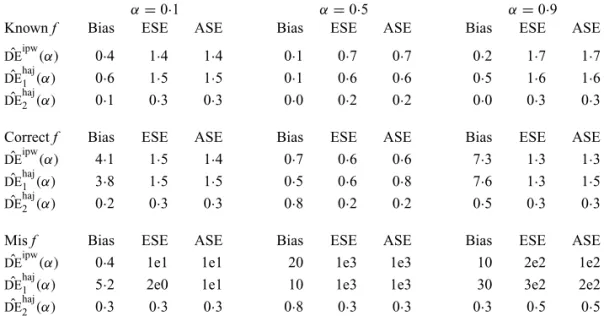
Table 1. Empirical bias (×10), empirical standard error, and average estimated standard error of the estimators of DE¯ (α)with a continuous outcome
α=0·1 α=0·5 α=0·9
Knownf Bias ESE ASE Bias ESE ASE Bias ESE ASE
ˆ
DEipw(α) 0·4 1·4 1·4 0·1 0·7 0·7 0·2 1·7 1·7 ˆ
DEhaj1 (α) 0·6 1·5 1·5 0·1 0·6 0·6 0·5 1·6 1·6
ˆ
DEhaj2 (α) 0·1 0·3 0·3 0·0 0·2 0·2 0·0 0·3 0·3 Correctf Bias ESE ASE Bias ESE ASE Bias ESE ASE
ˆ
DEipw(α) 4·1 1·5 1·4 0·7 0·6 0·6 7·3 1·3 1·3
ˆ
DEhaj1 (α) 3·8 1·5 1·5 0·5 0·6 0·8 7·6 1·3 1·5 ˆ
DEhaj2 (α) 0·2 0·3 0·3 0·8 0·2 0·2 0·5 0·3 0·3
Misf Bias ESE ASE Bias ESE ASE Bias ESE ASE
ˆ
DEipw(α) 0·4 1e1 1e1 20 1e3 1e3 10 2e2 1e2
ˆ
DEhaj1 (α) 5·2 2e0 1e1 10 1e3 1e3 30 3e2 2e2
ˆ
DEhaj2 (α) 0·3 0·3 0·3 0·8 0·3 0·3 0·3 0·5 0·5
ESE, empirical standard error; ASE, average estimated standard error; Knownf, true propensity score known; Correctf, propensity score unknown but correctly modelled; Misf, propensity score incorrectly modelled.
γ1Xvi1+γ2Xvi2+γ3Xvi3+γ4Xvi4+bv, whereXvi1 =exp(Lvi1/2),Xvi2 =Lvi2/{1+exp(Lvi1)}+1, Xvi3=(Lvi1Lvi3/1·5+0·6)3andXvi4=(Lvi1+Lvi4+2)2, were fitted to the simulated data.
Step 5. The causal effect estimators and their corresponding variance estimators were cal-culated for α1 = 0·1, 0·5, 0·9 andα0 = 0·1 using the known propensity score, the estimated propensity score from the correctly specified mixed-effects model and the estimated propensity score from the misspecified mixed-effects model.
Step6. Steps 1–5 were repeated 10 000 times, and the empirical bias, empirical standard error and average estimated standard error were calculated for the estimators in Step 5.
From the potential outcome model specified in Step 1 it follows thatμzα =5+3z+2(η−1)α and μα = 5+(2η+1)α where η = E(Nv2)/E(Nv). Hence DE¯(α) = 3 for any α ∈ (0, 1),
¯
IE(α1,α0)=2(η−1)(α1−α0),TE¯(α1,α0)=3+2(η−1)(α1−α0)andOE¯ (α1,α0)=(2η+1)(α1− α0). Simulation results for the direct effect estimators are given in Table1. All three estimators are approximately unbiased when the propensity scores are known or correctly modelled, but are biased if the propensity scores are incorrectly modelled. For all three estimators the average estimated standard error is also relatively close to the empirical standard error when the propensity scores are known or correctly modelled. Note thatDEˆ haj2 (α)has substantially smaller empirical
standard error thanDEˆ ipw(α)andDEˆ haj1 (α). For example, whenα =0·1 and the propensity scores
are known, the empirical standard errors of DEˆ ipw(α) and DEˆ haj1 (α) are 1·4 and 1·5, whereas
the empirical standard error of DEˆ haj2 (α) is only 0·3. Similar results hold when the propensity
scores are treated as unknown and either correctly or incorrectly modelled. The results in Table1
demonstrate that, as well as having smaller empirical standard error,DEˆ haj2 (α)may be more robust
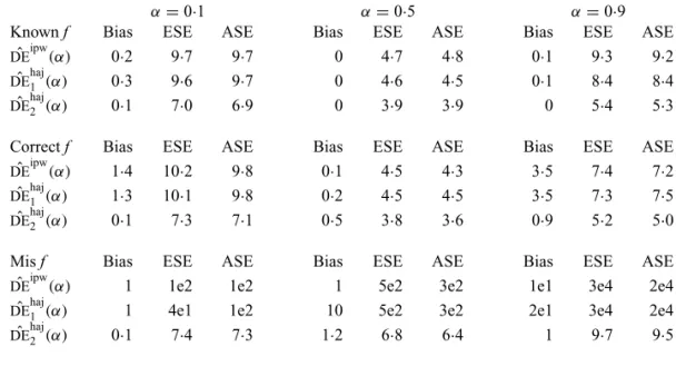
Table 2. Empirical bias, empirical standard error, and average estimated standard error of the estimators ofDE¯ (α)with a binary outcome; all values have been multiplied
by100
α=0·1 α=0·5 α=0·9
Knownf Bias ESE ASE Bias ESE ASE Bias ESE ASE
ˆ
DEipw(α) 0·2 9·7 9·7 0 4·7 4·8 0·1 9·3 9·2
ˆ
DEhaj1 (α) 0·3 9·6 9·7 0 4·6 4·5 0·1 8·4 8·4
ˆ
DEhaj2 (α) 0·1 7·0 6·9 0 3·9 3·9 0 5·4 5·3
Correctf Bias ESE ASE Bias ESE ASE Bias ESE ASE ˆ
DEipw(α) 1·4 10·2 9·8 0·1 4·5 4·3 3·5 7·4 7·2
ˆ
DEhaj1 (α) 1·3 10·1 9·8 0·2 4·5 4·5 3·5 7·3 7·5 ˆ
DEhaj2 (α) 0·1 7·3 7·1 0·5 3·8 3·6 0·9 5·2 5·0
Misf Bias ESE ASE Bias ESE ASE Bias ESE ASE
ˆ
DEipw(α) 1 1e2 1e2 1 5e2 3e2 1e1 3e4 2e4
ˆ
DEhaj1 (α) 1 4e1 1e2 10 5e2 3e2 2e1 3e4 2e4
ˆ
DEhaj2 (α) 0·1 7·4 7·3 1·2 6·8 6·4 1 9·7 9·5
The simulation study described above was repeated for a binary outcome. Specifically, Step 1 was replaced with the following, while all other steps remained the same.
Step 1. A random sample ofm = 500 groups was created as follows. First, the group size Nv was randomly sampled from{2, 3, 4, 5}with corresponding probabilities 1/8, 1/8, 1/2, 1/4.
Then the potential outcomesYvi(zvi,svi)were set to 0 with probability 0·2, 1 with probability 0·2,
and 1(Zvi=1,
Svi = |svi|) (v=1,. . .,m; i=1,. . .,Nv)with probability 0·6.
For this potential outcome model,μ1α =0·6λ+0·2,μ0α =0·2 andμα =0·6αλ+0·2 with λ=E(αNv−1Nv)/E(Nv). Simulation results for this scenario are given in Table2. Similar to the
continuous outcome simulations, the empirical standard error forDEˆhaj2 (α) is smaller than that
forDEˆ ipw(α)andDEˆ 1haj(α)in all three scenarios, andDEˆ haj2 (α)also tends to be more robust with
respect to misspecification of the propensity score model than the other two estimators. Similar results, not shown here, were observed for the other causal effect estimators.
6. ROTAVIRUS VACCINE STUDY IN NICARAGUA
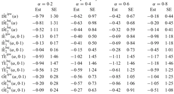
Table 3. Effect estimates for the rotavirus vaccine study; all values have been multiplied by10
α=0·2 α=0·4 α=0·6 α=0·8
Est SE Est SE Est SE Est SE
ˆ
DEipw(α) −0·79 1·30 −0·62 0·97 −0·42 0·67 −0·18 0·44
ˆ
DEhaj1 (α) −0·81 1·31 −0·63 0·98 −0·43 0·68 −0·20 0·45 ˆ
DEhaj2 (α) −0·52 1·11 −0·44 0·84 −0·32 0·59 −0·14 0·41
ˆ
IEipw(α, 0·1) −0·13 0·17 −0·40 0·50 −0·69 0·84 −0·98 1·18 ˆ
IEhaj1 (α, 0·1) −0·13 0·17 −0·41 0·50 −0·69 0·84 −0·99 1·18 ˆ
IEhaj2 (α, 0·1) −0·04 0·16 −0·15 0·45 −0·28 0·73 −0·45 1·01 ˆ
TEipw(α, 0·1) −0·93 1·46 −1·02 1·45 −1·11 1·45 −1·17 1·45 ˆ
TEhaj1 (α, 0·1) −0·94 1·47 −1·04 1·46 −1·12 1·46 −1·18 1·46 ˆ
TEhaj2 (α, 0·1) −0·56 1·25 −0·59 1·24 −0·61 1·25 −0·59 1·25 ˆ
OEipw(α, 0·1) −0·20 0·28 −0·56 0·73 −0·85 1·05 −1·04 1·25 ˆ
OEhaj1 (α, 0·1) −0·20 0·28 −0·57 0·73 −0·86 1·06 −1·05 1·25 ˆ
OEhaj2 (α, 0·1) −0·09 0·24 −0·27 0·63 −0·42 0·91 −0·51 1·08 Est, point estimate; SE, estimated standard error.
birth of study participants. Each individual in the study was visited fortnightly by a fieldworker for approximately one year. At each visit information about diarrhoea episodes in the past 14 days was recorded. The primary outcomeY was whether a child had at least one diarrhoea episode during the study.
For each child we assumed their interference set to be other children in the same household. A mixed-effects logistic regression model of the probability of having received all three scheduled doses was fitted conditional on the following baseline covariates: child’s age, categorized as 0– 11 months, 12–23 months, or 24–59 months; mother’s education level, categorized as primary education only or at least some secondary education; dirt household floor or not; dry or wet season; household indoor toilet, latrine, or none; indoor municipal water supply or not; and breastfeeding or not. Likelihood ratio tests from the fitted logistic model indicated that the odds of having all three doses of vaccine was higher among children whose mothers were more educated, with p=0·01.
Effect estimates and estimated standard errors are reported in Table3for the inverse probability-weighted and the two Hájek estimators for contrast function g(x1,x0) = x1−x0. The Hájek 2 estimates are closer to the null value of zero and, as expected, have 15–20% smaller estimated standard errors than the inverse probability-weighted and Hájek 1 estimates. The direct effect esti-mates indicate the expected difference in the proportions of children who will acquire rotavirus diarrhoea among vaccinated versus unvaccinated children for a fixed level of vaccine coverage
7. DISCUSSION
The inverse probability-weighted estimator and two Hájek-type estimators in §3allow for any form of interference between individuals, with the former being unbiased in a finite-population model with known propensity scores. Assuming partial interference and random sampling of groups from a superpopulation, all three estimators are consistent and asymptotically normal when the propensity scores are known or correctly modelled. Empirical results demonstrate that the second Hájek estimator can have substantially smaller finite-sample variance than the other two estimators. One avenue of future research entails deriving the estimators’ large-sample properties without assuming partial interference. Another future direction might involve devel-oping estimators which are robust with respect to misspecification of the propensity score model. Throughout this work conditional exchangeability is assumed, i.e., treatment is assumed to be independent of potential outcomes conditional on an observable set of covariates. In future work one could investigate relaxing this assumption, perhaps via sensitivity analysis or instrumen-tal variable methods. Finally, the target parameters in this paper utilize the Bernoulli allocation strategy proposed byTchetgen Tchetgen & VanderWeele(2012). These estimands consider the counterfactual scenario where individuals independently select treatment with equal probabil-ity. In scenarios where interference is present, it is unlikely that individual treatment selections would be independent. Therefore further interference-related research might target alternative parameters.
ACKNOWLEDGEMENT
The authors were partially supported by the U.S. National Institutes of Health. The fieldwork was supported by the Thrasher Research Fund. The content of this paper is solely the responsibility of the authors and does not necessarily represent the official views of the National Institutes of Health. The authors thank M. Elizabeth Halloran, Joseph Rigdon, an associate editor, and a reviewer for helpful comments.
APPENDIX
Proof of Proposition1
To show thatYˆipw(z,α)is unbiased, observe that
E{ ˆYipw(z,α)} =n−1
i
zi,si
yi(zi,si)1(zi=z)π(si;α)
f(zi,si|li,lχi)
f(zi,si|li,lχi)
=n−1
i
si
yi(z,si)π(si;α)= ¯y(z,α).
ThatYˆipw(α)is unbiased can be proved similarly.
Proof of Propositions2and3
To prove Proposition2, assume that there exist constantsc1,c2,c3 <∞andδ > 0 such that−c1 < Yvi<c2,Nv <c3,δ <f(Z˜v | ˜Lv)andδ <f(Zvi|Lvi)with probability 1. Letθˆ0= { ˆYipw(0,α),Yˆipw(1,α)}
andθˆh = { ˆYhaj
h (0,α),Yˆ
haj
h (1,α)}(h =1, 2). LetG
h(θ) = {Gh
0(θ),G
h
1(θ)}
T denote the vector estimating equationGh
α(Y˜v,Z˜v,L˜v;θ). LetG˙h(θ0)=∂Gh(θ0)/∂θ0Tand writev 2=v2
1+ · · · +v
2
pfor any vectorvof
lengthp.
First we show that the following four conditions hold for h = 0, 1, 2: (i) E{ ˙Gh(θ
0)} exists and
(iii) |∂2Gh
z(θ)/(∂θi∂θj)| ψ for some integrable measurable function ψ; and (iv)EGh(θ0)2 < ∞.
It is straightforward to show thatE{ ˙Gh(θ
0)} = −I2E(Nv), whereI2is the 2×2 identity matrix, implying
(i). Note that∂2Gh
z(θ)/(∂θi∂θj)=0, so (ii) holds and (iii) is satisfied for the functionψ=0. To show (iv),
observe that
EG0(θ0)2= 1
z=0 E
N v
i=1
Yvi1(Zvi=z)π(Svi;α)
f(Z˜v | ˜Lv)
−Nvμzα
2
.
From the boundedness assumptions onYvi,Nv andf(Z˜v | ˜Lv), it follows thatEG0(θ0)2 < ∞. Similar
results can be established forh=1, 2. Next, note that G0
zα(Y˜v,Z˜v,L˜v;μzα) is a linear function of μzα with slope −Nv. For h = 1, 2,
Gh
zα(Y˜v,Z˜v,L˜v;μzα)is also a linear function of μzα with finite, nonzero slope, because by assumption
f(Z˜v| ˜Lv) >0 and there exists at least oneisuch thatZvi=z. Hence, the solution forθto
m
v=1Gh(θ)=0
is unique forh =0, 1, 2. Therefore, because (i)–(iv) hold, by Theorem 5.4.2 ofvan der Vaart(1998),θˆh
converges in probability toθ0. Proposition2then follows from Theorem 5.4.1 ofvan der Vaart(1998) and
the delta method.
Similar reasoning can be used to prove Proposition3under the following additional assumptions about the parametric propensity score model:γ0is in an open subset of Euclidean space;E{ ˙G(γ0)}exists and
is nonsingular, whereG˙(γ0)=∂G(Z˜v,L˜v;γ0)/∂γ0T; G(z˜v,˜lv;γ )is twice continuously differentiable with
respect toγand|∂2G(z˜
v,˜lv;γ )/(∂γi∂γj)|ψfor some integrable measurable functionψfor every(z˜v,˜lv);
andEG(Z˜v,L˜v;γ0)2<∞.
Proof of reduction in variance with a correctly specified propensity score model
Using block matrix notation, write
U0∗= U0 Uμγ
0p×2 Uγ
, V0∗= V0 Vμγ VT
μγ Vγ
,
where 0p×2is thep×2 matrix of zeros. It is straightforward to show thatUγ = −Vγ andUμγ = −Vμγ. It
follows that
U0∗−1= U −1
0 −U0−1VμγVγ−1 0p×2 Uγ−1
and therefore
U∗−1 0 V0∗
U∗−1T
0
=
U0−1V0
U−1T
0
−U0−1VμγVγ−1VμγT
U−1T
0 ,
wheredenotes quantities not expressed explicitly. Hence
∗D
0 =
D
0 −τU−
1 0 VμγV−
1
γ VμγT
U−1T
0
τT
.
SinceVγ =E{G(Z˜v,L˜v;γ0)⊗2}is positive semidefinite, so isVγ−1. ThereforeD0 0∗D. The same approach
can be used to show thatD
h ∗
D
h forh=1, 2.
REFERENCES
ESPINOZA, F., PANIAGUA, M., HALLANDER, H., SVENSSON, L. & STRANNEGÅRD, Ö. (1997). Rotavirus infections in young Nicaraguan children.Pediatric Inf. Dis. J.16, 564–71.
HÁJEK, J. (1971). Comment on a paper by D. Basu. InFoundations of Statistical Inference, V. Godambe & D. Sprott, eds. Toronto: Holt, Rinehart and Winston, p. 236.
HALLORAN, M. E. & HUDGENS, M. G. (2012). Causal inference for vaccine effects on infectiousness.Int. J. Biostatist. 8, 1–40.
HALLORAN, M. E. & STRUCHINER, C. J. (1995). Causal inference in infectious diseases.Epidemiology6, 142–51. HONG, G. & RAUDENBUSH, S. W. (2006). Evaluating kindergarten retention policy: A case study of causal inference for
multilevel observational data.J. Am. Statist. Assoc.101, 901–10.
HORVITZ, D. G. & THOMPSON, D. J. (1952). A generalization of sampling without replacement from a finite universe.
J. Am. Statist. Assoc.47, 663–85.
HUDGENS, M. G. & HALLORAN, M. E. (2008). Toward causal inference with interference.J. Am. Statist. Assoc.103, 832–42.
LIU, L. & HUDGENS, M. G. (2014). Large sample randomization inference of causal effects in the presence of interference.J. Am. Statist. Assoc.109, 288–301.
LUO, X., SMALL, D. S., LI, C. S. R. & ROSENBAUM, P. R. (2012). Inference with interference between units in an fMRI experiment of motor inhibition.J. Am. Statist. Assoc.107, 530–41.
MANSKI, C. F. (2013). Identification of treatment response with social interactions.Economet. J.16, S1–23.
NICKERSON, D. W. (2008). Is voting contagious? Evidence from two field experiments.Am. Polit. Sci. Rev.102, 49–57. PEREZ-HEYDRICH, C., HUDGENS, M. G., HALLORAN, M. E., CLEMENS, J. D., ALI, M. & EMCH, M. E. (2014). Assessing
effects of cholera vaccination in the presence of interference.Biometrics70, 731–44.
ROSENBAUM, P. R. (2007). Interference between units in randomized experiments.J. Am. Statist. Assoc.102, 191–200. SOBEL, M. E. (2006). What do randomized studies of housing mobility demonstrate? Causal inference in the face of
interference.J. Am. Statist. Assoc.101, 1398–407.
STEFANSKI, L. A. & BOOS, D. D. (2002). The calculus of M-estimation.Am. Statistician56, 29–38.
TCHETGENTCHETGEN, E. J. & VANDERWEELE, T. J. (2012). On causal inference in the presence of interference.Statist.
Meth. Med. Res.21, 55–75.
van der VAART, A. (1998).Asymptotic Statistics. Cambridge: Cambridge University Press.
VANDERWEELE, T. J. & TCHETGENTCHETGEN, E. J. (2011). Effect partitioning under interference in two-stage randomized vaccine trials.Statist. Prob. Lett.81, 861–9.
VANDERWEELE, T. J., TCHETGENTCHETGEN, E. J. & HALLORAN, M. E. (2012). Components of the indirect effect in vaccine trials: Identification of contagion and infectiousness effects.Epidemiology23, 751–61.