6263.pdf

(1)

Modeling Dark Matter and Dark Energy

Kevin J. Ludwick

A dissertation submitted to the faculty of the University of North Carolina at Chapel Hill in partial fulfillment of the requirements for the degree of Doctor of Philosophy in the Department of Physics and Astronomy.

Chapel Hill 2013

Approved by:

Y. Jack Ng

Charles R. Evans

Reyco Henning

Dmitri Khveshchenko

(2)

(3)

Abstract

KEVIN J. LUDWICK: Modeling Dark Matter and Dark Energy. (Under the direction of Paul H. Frampton.)

We study various models of dark matter and dark energy. We first examine the

implications of the assumption that black holes act as dark matter. Assuming dark

matter in galactic halos is composed solely of black holes, and using observational

constraints, we calculate the number of halo black holes and the total entropy due

to them. We then study the prospect of dark energy with a non-constant density.

We analyze several parameterizations of dark energy density from the literature

and one of our own, in particular focusing on the value of redshift at which cosmic

acceleration due to dark energy begins. In considering the properties of dark

en-ergy densities that monotonically increase over time, we present two new

catego-rizations of dark energy models that we dub ”little rip” and ”pseudo-rip” models,

and both avoid future singularities in the cosmic scale factor. The dark energy

den-sity of a little rip model continually increases for all future time, and a pseudo-rip

model’s dark energy density asymptotically approaches a maximum value. These

two types of models, big rip models, and models that have constant dark energy

densities comprise all categories of dark energy density with monotonic growth

in the future. A little rip leads to the dissociation of all bound structures in the

universe, and a pseudo-rip occurs when all bound structures at or below a

cer-tain threshold dissociate. We present explicit parameterizations of the little rip

and pseudo-rip models that fit supernova data well, and we calculate the times at

which particular bound structures rip apart. In looking at different applications of

(4)

these models, we show that coupling between dark matter and dark energy with

an equation of state for a little rip can change the usual evolution of a little rip

model into an asymptotic de Sitter expansion. We also give conditions on

mini-mally coupled phantom scalar field models and scalar-tensor models that indicate

(5)

Acknowledgments

I am grateful to my advisor, Paul Frampton, for all his dedication, guidance, and

help throughout graduate school. I am thankful for all the members of my

com-mittee and the work they have done. I am also grateful to Robert Scherrer for his

collaboration in research and all the help he has offered me. I thank Shin’ichi Nojiri

and Sergei Odintsov for their collaboration in research. I appreciate all that Jack

Ng, Chris Clemens, and the rest of the physics department have done for me.

Many thanks to Mom, Dad, Jessica, Ryan, Nathan, and the rest of my family for

all their love, support, and good advice. I appreciate the long-time friendship of

Lee, Philip, and my apartment-mate Jeremy. I would not have eaten nearly as well

as I have over the past five years had it not been for the love, friendship, and and

excellent cooking of the Seniors (my second family), Teresa, the Tarltons, and the

Cuanies. And to others I did not mention here, thank you.

(6)

List of Figures

3.1 w(lin)₀ vs. w(lin)₁ . . . 30

3.2 w(CP L)₀ vs.w(CP L)₁ . . . 31

3.3 w(SSS)₀ vs. w(SSS)₁ . . . 31

3.4 w(new)₀ vs. w(new)₁ . . . 32

3.5 w(Z)vs.Z for all models . . . 33

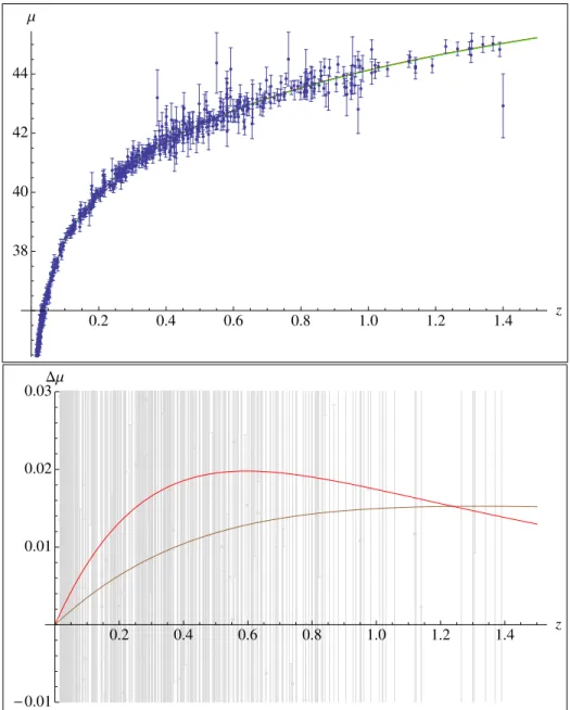
4.1 Hubble plot and Hubble residual plot . . . 47

6.1 ScaledFinertfor Model 1 . . . 77

(9)

List of Tables

2.1 Number of black holes with constraints from wide binaries . . . 20

2.2 Number of black holes without constraints from wide binaries . . . . 21

2.3 Entropy of black holes with constraints from wide binaries . . . 22

2.4 Entropy of black holes without constraints from wide binaries . . . . 22

(10)

Chapter 1 Introduction

1.1 Historical Background

Our universe is mysterious and wonderful. As we plumb deeper the depths of

space with our detectors and telescopes, the more we find that we do not

under-stand. Modern cosmology, the study of our universe’s origins, structure,

dynam-ics, and ultimate fate, has dramatically evolved from what it was in the early 1900s

to what it is today.

Soon after Einstein published his tensor equation describing general relativity

in 1915, he applied his equation to the universe in 1917, giving birth to relativistic

cosmology. His equation implied that the universe was expanding, and this

de-scription did not agree with the popular conception of the universe during his day.

So he added an extra term, often called the cosmological constant term, that was

consistent with the derivation of his equation, and this extra term ensured that his

equation described the universe as static [1]. As it turns out, the addition of the

cos-mological constant term gives a quasistatic solution that is unstable under

pertur-bations. Alexander Friedmann [2] and Georges Lemaˆıtre [3] independently wrote

down the solution to Einstein’s equation for a homogeneous and isotropic

(11)

realized that the solution gave a universe that started from a singularity. His

re-alization was the origin of the big bang theory, and it was not a widely accepted

one at that time. Later, Howard Percy Robertson [4] and Arthur Geoffrey Walker

[5], working independently in the 1930s, also worked out the solution for such

a universe. Their eponymous metric, the Friedmann-Lemaˆıtre-Robertson-Walker

(FLRW) metric, is the standard metric used in modern cosmology. Lemaˆıtre [3]

in 1927 and Edwin Hubble [6] in 1929, based on data from recession velocities of

galaxies, showed that the universe was, in fact, expanding. Hubble plotted the

re-cessional velocities of a set of galaxies versus their distance away from us, and he

made a linear fit. He deduced what is known as Hubble’s Law:v =H0d, wherevis

the velocity,dis the distance, andH0is the constant slope, known as Hubble’s

con-stant. The recessional velocity of galaxies and their distances away from us are not

related by a constant in time in general, but for the set of nearby galaxies Hubble

observed, a linear relationship with a constant slope of H0 is fairly accurate. The

idea of the big bang gained more popularity because of this evidence of expansion.

Einstein later said that adding the cosmological constant term to avoid expansion

was his biggest mistake. However, it turns out that the cosmological constant is

quite useful in describing dark energy, which we will discuss soon.

In response to the discovery of universal expansion, an alternative to the big

bang theory was proposed in the 1920s by Sir James Jeans, and his theory was

called the steady-state theory. In a steady-state universe, the universe has no

be-ginning or end, and new matter is continuously generated as the universe expands.

The FLRW metric follows the cosmological principle, which says that the universe

is homogeneous and isotropic on a large scale in space, but structure changes over

time as the universe expands. The steady-state universe follows the perfect

cos-mological principle, which says that the universe is homogeneous and isotropic in

(12)

spaceandin time. So a steady-state universe does not change its appearance over time. In 1948, a revised version of the steady-state model was promulgated by

Fred Hoyle, Thomas Gold, and Herman Bondi, among others. However, evidence

against this theory cropped up in the 1960s. Quasars and radio galaxies that were

far away from our galaxy were observed, but none were seen that were close to us.

This was a violation of the perfect cosmological principle.

For most, the final blow to the steady-state theory was the discovery of the

cosmic microwave background (CMB). In 1965, Arno Penzias and Robert Wilson

published their discovery of a uniform background of microwave radiation [7].

They had built a Dicke radiometer intended for experiments for satellite

com-munication. They discovered an excess in their antenna’s temperature that was

independent of the its orientation, and it was due to the CMB. The steady-state

model predicted discrete sources of background radiation from distant stars, but

the CMB gives off an almost perfectly uniform, blackbody spectrum. However,

the big bang theory very nicely predicts the existence of a microwave background

of radiation due to the decoupling of photons from electrons and protons as the

universe cooled over time. In fact, Ralph Alpher and Robert Herman predicted

in 1948 a cosmic microwave background of5 K [8], which is close to the modern

experimental value of2.72548±0.00057 K[9]. The CMB is not perfectly uniform; however, the anisotropies, which provide valuable insight into the formation of

our early universe and its structure, are well predicted by the big bang model

when augmented by inflation and quantum fluctuations of the inflaton field.

Shortly after the expansion of the universe was confirmed, Fritz Zwicky

no-ticed a discrepancy between mass measurements of galaxies in the Coma Cluster

in 1933. There was not enough luminous matter to account for the observed

(13)

concluded that there was missing mass, ”dark matter,” that accounted for the

un-expected observations [10]. In the 1960s and 1970s, Vera Rubin and others used

a new spectrograph that measured more accurately than ever before the rotation

curves of spiral galaxies, which show how fast stars orbit around the centers of

galaxies. Like Zwicky, she found an apparent violation of the virial theorem. The

stars near the edge of the spiral galaxies she observed were moving too fast to stay

bound to their galaxies according to the galactic masses measured from the visible

matter in them. In fact, she showed that about 50% of a typical spiral galaxy’s mass

is located beyond the radius containing the luminous galactic matter. She and her

collaborators published their results in 1980 [11].

Another milestone in cosmology recently happened when the High-z

Super-nova Search Team in 1998 [12] and the SuperSuper-nova Cosmology Project in 1999 [13]

published observations of the emission spectra of Type Ia supernovae indicating

that the universe’s rate of outward expansion is increasing. These groups found

that supernovae exhibited emission spectra that were redshifted more than

ex-pected from supernovae in a decelerating or zero-acceleration universe, so they

inferred that the universe was accelerating. Galaxy surveys and the late-time

inte-grated Sachs-Wolfe effect also give evidence for the universe’s acceleration. Thus,

”dark energy” was proposed as the pervasive energy in the universe necessary

to produce the ”anti-gravitational,” outward force that causes this acceleration,

which has been observationally tested and vetted since its discovery. The 2011

Nobel Prize in Physics was awarded to Schmidt, Riess, and Perlmutter for their

pioneering work leading to the discovery of dark energy.

(14)

1.2 Overview of Dark Matter and Dark Energy

About twenty-four percent of our universe is composed of dark matter, matter

that is electromagnetically undetectable because it does not emit any observable

amount of light. However, this non-luminous matter has been detected

gravita-tionally via gravitational lensing, and anisotropies in the CMB, examination of

baryonic acoustic oscillations (BAO), and structure formation simulations provide

good support for its existence.

Because dark matter is non-luminous, it is electromagnetically neutral. It is

also safe to say that particulate dark matter is not completely made up of baryonic

particles; otherwise, the CMB and comic structure formation would be drastically

different. Observational constraints on light elements created during big bang

nu-cleosynthesis, which strongly depend of baryon abundance [14], conflict with such

a theory. (There is some room for baryonic dark matter in the form of massive

com-pact halo objects (MACHOs), which will be discussed later.) Dark matter cannot be

completely composed of ”hot” particles, meaning particles that travel at relativistic

speeds. Light particles travel at ultrarelativistic speeds in the early universe and

stream through density perturbations, dampening them. One can relate the

small-est scale at which there is clumpy dark matter to the particle’s mass. Lyman-α

constraints suggest that a dark matter particle’s mass should be≥2keV [15]. There are many posited candidates for dark matter. Probably the most popular

candidate for cold (non-relativistic) dark matter is the Weakly Interacting Massive

Particle (WIMP). Such a particle was first proposed by Steigman and Turner [16],

and it interacts and has mass that is at the weak interaction scale. If such

par-ticles are in a thermal bath in the early universe and have an annihilation cross

(15)

equation agrees with the observational value for the number density of dark

mat-ter [17]. Some examples of WIMPs are the neutralino (motivated from

supersym-metry) and the Kaluza-Klein photon (motivated from theories with extra

dimen-sions). Other dark matter candidates include axion (proposed particles that solve

the strong CP problem), supersymmetric gravitinos, and dark matter from the

hid-den sector, which is a theoretical extension to the Standard Model comprised of

fields that have very little interaction with fields in the Standard Model. Another

candidate for dark matter is the leading warm dark matter candidate, the

ster-ile neutrino. Proponents argue that this model leads to more accurate structure

formation than cold dark matter does [18, 19]. Typical examples of the

aforemen-tioned MACHOs, which were originally proposed as objects that explained the

presence of non-luminous matter in galaxy halos, include neutron stars and black

holes. Primordial black holes (PBHs) and ultra-compact minihalos (UCMHs) are

more recent dark matter candidates. They may be classified as non-baryonic

MA-CHOs, and they form via the collapse of density perturbations near the time of the

big bang [20, 21, 22].

Instead of accounting for dark matter with extra matter, we can also try

mod-ified gravity models (e.g., f(R) gravity, scalar-tensor theories, Brans-Dicke

the-ories, braneworld gravity). Another attempt of modifying gravitational laws is

called Modified Newtonian Dynamics (MOND). The challenge for such models is

to correctly describe both structure formation and galaxy rotation curves. For

ex-ample, MOND is consistent with galaxy rotation curves, but it has more trouble

with structure formation.

It is a bit surprising that the amount of baryonic matter in the universe is

dwarfed by six times as much dark matter. Perhaps even more unsettling is the

presence of dark energy in our universe, which makes up the biggest portion,

(16)

about three quarters, of our universe.

However, our physical intuition of the nature and dynamics of dark energy

is severely lacking. For a fixed amount of normal matter, as the volume

contain-ing it increases, the density of the matter for the whole volume should decrease.

However, the nature of dark energy is counterintuitive in that its density remains

constant (or even increases) over time as the universe expands.

Many explanations for cosmic acceleration have been theorized. The varied

ap-proaches include modified gravity, adding an extra component for dark energy to

the components of mass/energy in the universe, and cosmological back-reaction,

which refers to the scenario in which inhomogeneity in the universe accounts for

cosmic acceleration. The standard explanation attributes dark energy to vacuum

energy that permeates the universe and is constant over time. The model that

ac-companies this explanation is called the cosmological constant model, named after

the extra term Einstein added into his equation to give a static universe. Einstein’s

equation can be derived with an extra term that is a constant times the metric (the

speed of lightc= 1throughout):

Rµν−

1

2Rgµν + Λgµν = 8πGTµν. (1.1)

Rµν is the Ricci tensor,Ris the Ricci scalar (the contracted Ricci tensor),gµν is the

metric, andTµνis the stress-energy tensor, which contains all the information about

the mass/energy contents of spacetime. The first two terms on the lefthand side of

the equation are the usual terms from Einstein’s equation representing the

curva-ture of spacetime. The third, extra term is the contribution of vacuum dark energy,

and the constant multiplier,Λ, is called the cosmological constant. Quantum field

(17)

cosmological value by an appalling 120 orders of magnitude, the largest

discrep-ancy between theory and experiment in all of physics. Perhaps the correct theory

of quantum gravity or some other theory will explain this inconsistency, and many

explanations have been proffered, for example, based on the string landscape and

the anthropic principle. It is a mystery for now.

The FLRW metric, mentioned previously, is

ds2 =−dt2 +a(t)2

dr2

1−kr2 +r

2₍_dθ2_{+ sin}2_θdφ2₎

, (1.2)

wherea(t)is the scale factor controlling the rate at which the universe expands/contracts,

andk determines the spatial curvature of the universe. Observations have shown

that the universe is almost completely spatially flat, i.e., k is very close to 0, so it

is usually set to0(and we usek = 0throughout this work unless otherwise

spec-ified). The spatial coordinatesr, θ, andφare comoving coordinates, meaning that

they move with the expansion/contraction of spacetime. For example, an object

that has no net force acting on it will have a constant comoving distance from the

origin,r, since it is moving only due to the expansion of the universe. The proper

distance of that object from the origin at time t isa(t)r, which changes in time in

accordance with the expansion of spacetime. By solving Einstein’s equation using

the spatially flat FLRW metric and modeling the contents of the universe as a

ho-mogeneous, perfect fluid, we can obtain the Friedmann equations (which bear the

name of the previously mentioned Alexander Friedmann):

˙

a a

2

= 8πG

3 ρ (1.3)

¨

a a =−

4πG

3 (ρ+ 3p). (1.4)

(18)

The dot overadenotes a derivative with respect to time,ρis the total density of the

mass/energy contents of the universe, andpis the fluid pressure of these. Notice

that there is no spatial dependence in these equations; this is because we

origi-nally assumed isotropy and homogeneity in our universe. These equations are

sometimes written in terms of the Hubble parameter, which is the generalization

of Hubble’s constant for any time: H ≡ a˙ a.

The cosmological constant term is usually subsumed as an extra component of

the density in the stress-energy tensor as in the following:

ρ=X

i

ρi =ρrad+ρm+ρΛ, (1.5)

where the first term is the contribution from radiation from photons and

ultrarel-ativistic neutrinos, the second term from baryonic and dark matter, and the third

term from the constant vacuum energy. Another way of expressing the

compo-nents of mass/energy is

1 =X

i

Ωi(t) = Ωrad(t) + Ωm(t) + ΩΛ(t), (1.6)

whereΩi(t)for a flat metric isρ_ρ(t)i(t). The sum of all the fractions of the total mass/energy

in the universe at a given time adds up to1for a flat universe. (Sometimes, Ωi is

used to indicate the present-day value ofΩi(t)in the literature.) Usually, the

equa-tion of state of a perfect fluid component in the stress-energy tensor is modeled as

pi =wiρi. (1.7)

For the cosmological constant model,wΛ=−1, and the dark energy density is

con-stant only if this is the case. A universe that contains only the vacuum energy from

(19)

who found such a solution to Einstein’s equation using his cosmological constant

term [23]. We usually generalizewΛto bewDE, which is not restricted to be −1. A

troubling facet of dark energy modeled as a perfect fluid is that it necessarily

vi-olates the strong energy condition of general relativity. The energy conditions are

meant to loosely dictate what kinds of matter/energy are acceptable and physical.

For a perfect fluid, they are as follows:

weak energy condition (WEC) : ρ≥0, ρ+p≥0 (1.8)

null energy condition (NEC) : ρ+p≥0 (1.9)

strong energy condition (SEC) : ρ+p≥0, ρ+ 3p≥0 (1.10)

dominant energy condition (DEC) : ρ≥ |p|. (1.11)

The cosmological constant model violates the SEC (and not the other energy

con-ditions). We know from observations that our universe during the present epoch is

dominated by dark energy, so we can approximateρ ≈ ρDE. From equation (1.4),

we see that¨a (representing acceleration) is positive only ifρ+ 3pis negative, i.e.,

ifw ≤ −1/3. Thus, dark energy as a perfect fluid violates the SEC. (This violation can be shown without assuming ρ ≈ ρDE, but we make the assumption for the

sake of simplicity.) On the other hand, ifρ < 0and w = −1, thenp > 0, and the SEC is preserved. But then ¨a is not positive, so there is no cosmic acceleration,

and the DEC and WEC are violated. However, the most recent observational value

of wmade by the Nine-Year Wilkinson Microwave Anisotropy Probe (WMAP 9)

combining data from WMAP, the CMB, BAO, supernova measurements, andH0

measurements, is w = −1.037+0.071₋_0.070 at the 95% confidence level [24], assuming a perfect fluid for dark energy, a constant value of w, and a flat universe (which

is a good assumption based on observations). So the cosmological constant (CC)

(20)

model is in good agreement with observation, and it also agrees with the similar

observational value ofwwhen the universe is not assumed to be flat. In fact, the

best fit value forwis less than−1, even though all energy conditions are violated for dark energy with w < −1 according to equations (1.8) - (1.11). When com-bined with WMAP polarization and supernova data, the very latest cosmological

data, from the Planck satellite, gives w = −1.13+0.013₋_0.14 at the 95% confidence level [25], and the CC model is just barely preserved for this data set. Dark energy with

w < −1 is known as phantom dark energy, and its density increases over time. Therefore, observations seem to indicate that preserving the SEC and other energy

conditions may not be so important. General relativity has not been tested past the

scale of our solar system, whereas all the observations that led to this best fit value

ofwwere very far beyond that scale.

Many theoretical dark energy models have been found that are within

observa-tional constraints, and many of these models allowwDE to be a function that can

change over time. One such form of dynamical dark energy modeled with a scalar

field is called quintessence. The equation of motion for the scalar field, which

fol-lows from local conservation of mass/energy and momentum,∇µTνµ = 0 (which

follows from Einstein’s equation), is

∇µ∇µφ+

∂V

∂φ = 0, (1.12)

where V(φ)is the scalar field potential. Assuming the scalar field is spatially

ho-mogeneous (∂µφ∂µφ = ˙φ2), The fluid density and pressure of the scalar field are

ρφ=

1 2

˙

φ2₊_V₍_φ₎_, _p φ =

1 2

˙

φ2₋_V₍_φ₎_. _(1.13)

(21)

Quintessence theories with a negative, non-standard kinetic term are aptly called

k-essence theories. Because of the negative kinetic term, the field ”rolls up” the

potential. Phantom field theories are a bit troublesome since they have ”ghosts,” or

vacuum instabilities. However, these problems can be avoided if they are treated

as effective field theories that have momentum cutoffs [26, 27]. And as we have

already seen, phantom models seem to be supported by observation, so perhaps

such theories will be fleshed out better in the future as we learn more about the

nature of dark energy.

1.3 Motivation and Plan of this Work

Cosmologists have come a long way in understanding dark matter and dark

en-ergy and their observational constraints, but there are still many unanswered

ques-tions. There are still several plausible explanations of these two phenomena.

In chapter two, we explore the possibility of intermediate-mass black holes

(IMBHs) comprising all of dark matter. IMBHs typically range in mass from about

103 _- ₁₀5_M

. One aspect of this approach that is beneficial in the interest of

ef-ficiency and simplicity is that the introduction of new, unknown particles is not

necessary. Black holes are reasonably well understood objects that have

theoret-ical and observational grounding; for example, it is widely accepted from

obser-vations that supermassive black holes reside in the center of galaxies. Based on

constraints from microlensing and galactic disk stability, both with and without

limitations from wide binary surveys, we estimate the total number and entropy

of intermediate-mass black holes. Given that the visible universe comprises 1011

halos each of mass∼ 1012_M

, typical core black holes of mean mass∼ 107M set

the dimensionless entropy (S/k) of the universe at a thousand googols (1googol

= 10100_{). One interesting feature of this dark matter candidate is that the entropy}

(22)

contribution from these IMBHs can exceed that of supermassive black holes in

the universe, which are presently the biggest known contributor to the universe’s

entropy. Identification of all dark matter as black holes allows a dimensionless

entropy of the universe up to ten million googols, implying that dark matter can

contribute over 99% of entropy. If we hypothesize that, for some dynamical

rea-son, the entropy of the universe is maximized, this favors all dark matter as black

holes in the mass regime of∼105_M

.

Chapter three concerns our investigation of dark energy models with

non-constant densities. Since such models could possibly describe dark energy, we

think it is important to study the dynamics and properties of such models. We

study how to distinguish between a cosmological constant and evolving dark

en-ergy with equation of state w(Z), where Z is the redshift. Redshift is defined as

Z = λobserved

λemitted

−1, (1.14)

whereλobserved is the observed wavelength of light from an object in question and

λemittedis the wavelength of light emitted. So we detect light that is longer in

wave-length (lower in frequency, toward the red end of the electromagnetic spectrum)

than that of the original emitted light from an object that is moving away with

the expansion of the universe. This effect is somewhat analogous to the Doppler

shift. Redshift happens due to the stretching of space, and it happens according to

the FLRW metric of spacetime. Redshift due to the expansion of the universe from

timetin the past to the present time relates to the scale factor in the following way:

Z = a(t)

a(t0)

−1. (1.15)

t0 is defined to be the present time, anda(t0), also written asa0, is usually taken to

(23)

In chapter three, we focus on the value of redshift Z∗ at which cosmic

accel-eration begins, which means that ¨a(Z∗) = 0. Four w(Z) are studied, including

the well-known CPL model and a new model that has advantages when

describ-ing the entire expansion era. If dark energy is represented by a CC model with

w = −1, Z∗ is about 0.7. We discuss the possible implications of a more accurate, model-independent measurement ofZ∗.

In 2002, Robert Caldwell [28, 29] explored dark energy models with constant

wDE < −1, phantom dark energy models. The CC model leads to a constant

cosmic acceleration, and thus dark energy provides a constant force on the

uni-verse. But for phantom models, the cosmic acceleration is increasing over time.

So if the cosmic force due to dark energy gets big enough to overcome the forces

holding together bound structures such as galaxies, solar systems, and even the

smallest atoms, these structures can be ripped apart in the future. For phantom

models, the scale factoraand ρDE approach infinity at a finite time in the future.

Caldwell called such a fate of the universe a ”big rip.” Chapter four focuses on a

particular fate of the universe we have dubbed the ”little rip.” A little rip model

features a dark energy density that increases with time (so that wDE(a) satisfies

wDE(a) < −1), butwDE approaches−1asymptotically, and there is no future

sin-gularity. We discuss conditions necessary to produce this evolution. Such

mod-els can display arbitrarily rapid expansion in the near future, leading to the

de-struction of all bound structures. We determine observational constraints on two

specific parameterizations and calculate the point at which the disintegration of

certain bound structures begins. For the same present-day value ofwDE, a big rip

with constantwDE disintegrates bound structures earlier than a little rip.

Manifestations of little rip models can be via parameterizations ofρDE, k-essence

models, scalar-tensor theories, and models in which dark energy and dark matter

(24)

are coupled. We employ all of these in chapter five.

A scalar-tensor theory is simply a theory in which gravity is described by the

action of a scalar field along with the usual tensor field of general relativity. One

such model we examine in chapter five is given by the action

S =

Z

d4x√−g

1 16πGR−

1

2ω(φ)∂µφ∂

µ_φ₋_V₍_φ₎

, (1.16)

where g is the determinant of the metric,R is the Ricci scalar, andω(φ)and V(φ)

are functions of the field φ. V(φ) is the scalar field potential, and dark energy

is represented by φ. Without the second and third terms, minimizing the action

would result in Einstein’s equation for an empty universe, i.e., for a stress-energy

tensor Tµν = 0. We leave out terms for matter and radiation because we consider

this model only when dark energy dominates over other density components, so

these terms are negligible.

Usually, different density components are considered independent of each other,

but we consider the coupling of dark energy and dark matter, which, given our

rel-ative ignorance of the nature of these two, is plausible. Combining the two

Fried-mann equations, equations (1.3) and (1.4), we can obtain the continuity equation:

˙

ρ=−3(ρ+p)a˙

a ⇒ dρ da =−

3

a(ρ+p). (1.17)

ρand pcan be written as the sum of their components, and if each component is

independent of the others, then

X i

dρi

da =−

X i

3

a(ρi+pi) ⇒ dρi

da =−

3

(25)

for eachi. This implies

ρrad(a) =ρrad0a

−4 _, _ρ

m(a) =ρm0a

−3_,

(1.19)

where ρi0 ≡ ρi(a0). The pressure due to a relativistic fluid isprad =

ρrad

3 , and cold

(non-relativistic) matter is without pressure. From these functional forms forρrad

and ρm, it is clear that radiation dominated the early universe (for small a). As

the universe cooled more, matter began to dominate the evolution of the universe,

thusρm(a)took over when abecame large enough. We study the implications of

the coupling between dark matter and dark energy so that the continuity equation

for these components are not separable.

Also in chapter five, we derive the conditions for the little rip in terms of the

force due to dark energy and present two representative models to illustrate the

difference between little rip models and those which are asymptotically de Sitter.

We derive conditions onwDEto distinguish between the two types of models. The

coupling between dark matter and dark energy with an equation of state that leads

to a little rip can alter the evolution, changing the little rip into an asymptotic de

Sitter expansion. We give conditions on minimally coupled phantom scalar field

models (k-essence models) and on scalar-tensor models that indicate whether or

not they correspond to a little rip expansion. We show that, counterintuitively,

despite local instability the previously discussed [26, 27], a little rip has an infinite

lifetime.

If we assume that the cosmic energy density will remain constant or strictly

increase (i.e., monotonically increase) in the future, then the possible fates for the

universe can be divided into four categories based on the time asymptotics of the

Hubble parameterH(t). Three of the categories, which we have already discussed,

are the following: the cosmological constant, for which H(t) = constant; the big

(26)

rip, for whichH(t)goes to infinity at finite time; and the little rip, for whichH(t)

goes to infinity as time goes to infinity. In chapter six, we introduce the fourth

cat-egory, which we call the ”pseudo-rip.” For a pseudo-rip, H(t) goes to a constant

as time goes to infinity, which is an intermediate case between the cosmological

constant and the little rip. Because of equation (1.3), ”H(t)” can be replaced with

”ρ” in these four conditions. In chapter six, we provide models that exemplify the

pseudo-rip and that fit observational data well. Structures with a binding force

at or below a threshold determined by the model’s parameters will dissociate. We

show that pseudo-rip models for which the density and Hubble parameter increase

monotonically can produce an inertial force which does not increase

monotoni-cally, but instead peaks at a particular future time and then decreases.

In chapter seven, we conclude and discuss future possible applications and

(27)

Chapter 2 Number and Entropy of Black Holes

1

2.1 Introduction

The identification of dark matter, for which there is compelling evidence from its

gravitational effects in galaxies and clusters thereof, is an important outstanding

question. Dark matter makes up some eighty percent of matter and a quarter of

the energy content of the universe.

Of course, it would be reassuring to identify dark matter by its production in

particle colliders and by its detection in terrestrial experiments. On the other hand,

the dark matter constituent may equally be, as assumed here, in a completely

dif-ferent and collider-inaccessible mass regime heavier than the Sun.

The observational limits on the occurrence of such multi-solar mass

astrophysi-cal objects in the halo have considerably changed recently. There remain

microlens-ing limits [31, 32] on masses below a solar mass and slightly above. There are also

respected limits from numerical study [33] of disk stability at ten million solar

masses and slightly below.

(28)

For the intermediate-mass region, a possible constraint comes from the

occur-rence of gravitationally bound binary stars at high separation approaching one

parsec. Here the situation has changed recently, and the bounds are far more

re-laxed, possibly non-existent. The first such analysis [34] allowed only some ten

percent of halo dark matter for most of the mass range. A more recent analysis [35]

permits fifty perecent and cautions that the sample of binaries may be too small to

draw any solid conclusions.

In the following, we adopt constraints from microlensing and disk stability but

keep an open mind with respect to the wide binaries. We estimate the total number

and total entropy of the black holes per halo and hence (simply multiplying by

1011) in the universe, assuming as in [36] that all dark matter can be identified as black holes.

2.2 Number of Black Holes

To estimate number and subsequently entropy of black holes we simplify by taking

as possible masses 10n_M

with n integer, 1 ≤ n ≤ 7. Further, we assume the

constraints from wide binaries [35] for differentnare independent of each other.

We make our analysis first with binary constraints, denoted simply as “with”,

then with no binary constraints, denoted as “without”. Let fn be the fraction of

the halo dark matter composed of mass10nMblack holes. The total halo mass is

taken to be1012M whereupon

Σnfn = 1 (2.1)

and the numberNnis

(29)

The “with” constraints on thefnare

0 ≤ f1 ≤0.4

0 ≤ f2 ≤1.0

0 ≤ f3 ≤0.5

0 ≤ f4,5,6 ≤0.4

0 ≤ f7 ≤0.3. (2.3)

For the “without” constraints, the f1,2,7 ranges remain unchanged while the

f3,4,5,6 are free, namely

0 ≤ f1 ≤0.4

0 ≤ f2,3,4,5,6 ≤1.0

0 ≤ f7 ≤0.3. (2.4)

Allowing thefnto vary by increments∆fn = 0.1for1≤fn≤(fn)maxwe allow

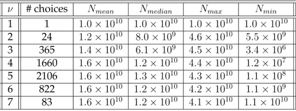
the black holes to have ν different mass (or n) values with 1 ≤ ν ≤ 7. For the “with” constraints, we then find numbers of black holes as follows:

ν # choices Nmean Nmedian Nmax Nmin

1 1 1.0×1010 1.0×1010 1.0×1010 1.0×1010 2 24 1.2×1010 ₈_.₀_×₁₀9 ₄_.₆_×₁₀10 ₅_.₅_×₁₀9

3 365 1.4×1010 ₆_.₁_×₁₀9 ₄_.₅_×₁₀10 ₃_.₄_×₁₀6

4 1660 1.6×1010 ₁_.₂_×₁₀10 ₄_.₄_×₁₀10 ₁_.₂_×₁₀7

5 2106 1.6×1010 1.3×1010 4.3×1010 1.1×108 6 822 1.6×1010 ₁_.₂_×₁₀10 ₄_.₂_×₁₀10 ₁_.₁_×₁₀9

7 83 1.6×1010 ₁_.₂_×₁₀10 ₄_.₁_×₁₀10 ₁_.₁_×₁₀10

Table 2.1: Number of black holes with constraints from wide binaries.

For the “without” case we find:

(30)

ν # choices Nmean Nmedian Nmax Nmin

1 5 2.2×109 ₁_.₀_×₁₀9 ₁_.₀_×₁₀10 ₁_.₀_×₁₀6

2 125 6.1×109 ₉_.₀_×₁₀8 ₄_.₆_×₁₀10 ₇_.₃_×₁₀5

3 890 1.0×1010 4.0×109 4.5×1010 1.6×106 4 2340 1.4×1010 ₁_.₀_×₁₀10 ₄_.₄_×₁₀10 ₁_.₁_×₁₀7

5 2346 1.5×1010 ₁_.₂_×₁₀10 ₄_.₃_×₁₀10 ₁_.₁_×₁₀8

6 840 1.6×1010 1.2×1010 4.2×1010 1.1×109 7 83 1.6×1010 1.2×1010 4.1×1010 1.1×1010

Table 2.2: Number of black holes without constraints from wide binaries.

Study of Tables 1 and 2 reveals a number of things about the putative

intermediate-mass black holes which may dominate the matter content. First, the comparison

of the tables reveals that the wide binary constraints, as they stand, do not affect

the numbers very much. Thus, unless and until a much bigger sample of wide

binaries is found (if they exist), the conclusions about numbers of black holes in a

halo is insentive to their consideration.

As expected from the defining formula, Eq. (2.2), the number of black holes

per halo can range from about a million to a few times ten billion. By sampling

distributions of the masses, not just a single mass, Tables 1 and 2 reveal that the

most likely number is at the high end, close to ten billion per halo.

Since there are generically 1011 halos, this implies a total number of about a billion trillion black holes in the universe.

2.3 Entropy of Black Holes

We can similarly estimate the total entropy of the halo black holes by exploiting

the Parker-Bekenstein-Hawking entropy formula [37, 38, 39], which says that for a

black hole with massMBH =ηM, the entropy isSBH = 1078η2.

(31)

ν # choices Smean Smedian Smax Smin

1 1 1.0×1092 ₁_.₀_×₁₀92 ₁_.₀_×₁₀92 ₁_.₀_×₁₀92

2 24 3.0×1095 ₇_.₁_×₁₀93 ₃_.₀_×₁₀96 ₆_.₄_×₁₀91

3 365 7.5×1095 2.2×1995 3.4×1096 1.5×1092 4 1660 1.1×1096 ₁_.₀_×₁₀96 ₃_.₄_×₁₀96 ₁_.₁_×₁₀93

5 2106 1.4×1096 ₁_.₂_×₁₀96 ₃_.₄_×₁₀96 ₁_.₁_×₁₀94

6 822 1.5×1096 1.2×1096 3.3×1096 1.1×1095 7 83 1.6×1096 1.2×1096 3.2×1096 1.1×1096

Table 2.3: Entropy of black holes with constraints from wide binaries.

while for the “without” case we find

ν # choices Smean Smedian Smax Smin

1 5 2.2×1095 1.0×1095 1.0×1096 1.0×1092 2 125 4.5×1095 ₈_.₀_×₁₀94 ₃_.₇_×₁₀96 ₆_.₄_×₁₀91

3 890 7.7×1095 ₃_.₀_×₁₀95 ₃_.₆_×₁₀96 ₁_.₅_×₁₀92

4 2340 1.1×1096 1.0×1096 3.5×1096 1.1×1093 5 2346 1.3×1096 ₁_.₂_×₁₀96 ₃_.₄_×₁₀96 ₁_.₁_×₁₀94

6 840 1.5×1096 ₁_.₂_×₁₀96 ₃_.₃_×₁₀96 ₁_.₁_×₁₀95

7 83 1.6×1096 ₁_.₂_×₁₀96 ₃_.₂_×₁₀96 ₁_.₁_×₁₀96

Table 2.4: Entropy of black holes without constraints from wide binaries.

Tables 3 and 4 contain much information germane to the central idea that dark

matter be identified as black holes.

The biggest known contributor of black holes in a halo is the core supermassive

black hole (SMBH). In the Milky Way it is Sag A* and for a typical galaxy a core

SMBH has mass MSM BH ∼ 107M. Its Parker-Benkenstein-Hawking entropy is

therefore about∼1092.

Multiplying by1011_{, the number of halos, shows that these SMBHs contribute}

about 10103_{, or a thousand googols, to the entropy of the universe as emphasized}

in [36].

The conventional wisdom is that the SMBHs are the single dominant

contribu-tor to the entropy of the universe, which is therefore about a thousand googols.

(32)

From our Tables 3 and 4 we can arrive at a very different conclusion.

2.4 Reconsideration of the Entropy of the Universe

Let us take the viewpoint that the universe, by which we mean the visible universe,

is an isolated system in the usual sense of thermodynamics and statistical

mechan-ics. In accord with the usual statistical law of thermodynamics, the entropy of the

universe will increase to its maximum attainable value.

The natural unit for the dimensionless entropy of the universeS/k= ln Ωis the

googol (10100_{). The supermassive black holes (SMBHs) at galactic cores contribute}

about a thousand googols.

The holographic bound [40] on information or entropy contained in a

three-volume is that it be not above the surface area as measured in Planck units(10−33_cm2_).

If we take the visible universe to be a sphere of radius3×1010ly ∼3×1018cm, the maximum entropy is ∼ 10124 or a trillion trillion googols. This would be the en-tropy if the universe were one black hole of mass1023_M

.

The numbers in Tables 3 and 4 suggest that the entropy contribution from dark

matter can exceed that of the SMBHs by orders of magnitude. Taking the view that

increasing total entropy plays a dominant role in cosmological evolution strongly

favors the formation of black holes in the105_M

mass range and the view that they

constitute all dark matter.

We are more confident about the present status of dark matter than of its

de-tailed history but, of course, an interesting and legitimate question is: how did

the black holes originate? One possible formation is as remnants of Population-III

(henceforth Pop-III) stars formed at a redshiftZ ∼ 25. These Pop-III stars are nec-essary to explain the metallicity of Pop-I and Pop-II stars that formed later. Such

(33)

105_M

, to live for a short time, less that a million years, then explode leaving black

holes which have a total mass that is a significant fraction of the original star’s

mass. Nevertheless, it is very unlikely [41] that a sufficient number of Pop-III stars

can form to make all dark matter. Thus, the IMBHs may have formed in the early

universe as primordial black holes.2

The first item of business is therefore to confirm that there are millions of large

black holes in our halo and in others.

The ESA Gaia project is planned to survey billions of stars in our galaxy, the

Milky Way, and should enable obtaining a large sample of gravitationally bound

wide binaries which can be analyzed for evidence of black holes perturbing them.

The goal of the SuperMACHO project is to identify the objects which produced

existing microlensing events and should allow the observation of higher longevity

microlensing signals corresponding to the mass ranges suggested for the dark

mat-ter black holes.

Finally, if we truncate ton ≤5, since Pop-III stars or IMBHs with higher masses seem unlikely [41], then the typical number of IMBHs per halo is ∼ 1010, giving about one million googols for the entropy of the universe. The majority of entropy

may be concentrated in a tiny fraction of the total number of black holes as can be

seen by studying examples, e.g.,f2 =f5 = 0.5.

The key motivation for our believing this interpretation of dark matter, as

op-posed to an interpretation involving microscopic particles, comes from

considera-tion of the entropy of the universe. The SMBHs at galactic cores contribute about

a thousand googols to the overall dimensionless entropy. As seen in the present

article, dark matter in the form of black holes can contribute as much as a million

2_{Note that the constraints in [21] apply at the recombination era and subsequent black hole}

mergers can occur.

(34)

googols and thus make up over99%of the cosmic entropy, which is sufficient

rea-son, if we adopt that the universe is an isolated system to which the second law of

thermodynamics is applicable, for taking it seriously.

Hopefully future observations will be able to identify dark matter as black

(35)

Chapter 3 Seeking Evolution of Dark Energy

1

3.1 Introduction

The interface between astrophysics and particle physics has never been stronger

than now because our knowledge of gravity comes in large part from observational

astronomy and cosmology. At particle colliders, seeking the constituent of dark

matter is an important target of opportunity.

Dark energy is widely regarded as the most important issue in all of physics

and astronomy. Other than the cosmological constant (CC) model, and the very

interesting, if not yet fully satisfying, usage of string theory, there is no compelling

theory. So we are motivated to pursue a purely phenomenological approach to

attempt to make progress towards the understanding of dark energy.

The discovery of cosmic acceleration [13, 12] in 1998 has revolutionized

theo-retical cosmology. The simplest theotheo-retical interpretation is as a CC with constant

density and equation of state (EoS)w≡ −1. We shall refer to alternatives to the CC model, withw(Z)redshift-dependent, as evolutionary dark energy.

(36)

The equations which govern cosmic history, which assume Einstein’s

equa-tions, isotropy, homogeneity (FLRW metric [2, 3, 4, 5]), and flatness as expected

from inflation, are (withc= 1):

H(t)2 =

˙ a a 2 = 8πG 3 ρ (3.1) and ¨ a a

=−4πG

3 (ρ+ 3p), (3.2)

together with the continuity equation:

adρ

da =−3(ρ+p). (3.3)

In these equations, p is pressure and ρ is the density with components ρ =

ρΛ+ρm+ργ. Although, for small redshifts, the radiation term is by far the smallest,

we still include it.

Using Eq. (3.2), the CC model withw≡ −1, and the WMAP7 values2

ΩΛ(t0) = 0.725±0.016 and Ωm(t0) = 0.274±0.013, (3.4)

we find that [44]

Z∗ =

2ΩΛ(t0)

Ωm(t0) 1₃

−1 = 0.743±0.030. (3.5)

With evolution, Eq. (3.5) is modified. It is worth mentioning that Z∗ is a

constant of Nature, like Hubble’s constant, which can in principle be measured

2_{Note that we use the WMAP7 [43] value for}_Ω

m(t0), unless explicitly stated otherwise. We use

(37)

precisely, without reference to any theoretical model. We shall introduce various

evolutionary models, including the very popular CPL model [45, 46] w(CP L)(Z) and a new proposal w(new)(Z) that is more physically motivated with respect to the whole expansion history3_{. We present figures which make predictions for}_Z∗

,

and we suggest slowly varying criteria which support the use of w(new)₍_Z₎ _over

w(CP L)₍_Z₎_.

3.2 Evolutionary Dark Energy Models

When we consider dark energy models, we must specify an equation of statew(Z).

There is an infinite number of choices forw(Z): our objective in the present article

is to suggest a sensible choice for the functional form ofw(Z), which can be valid

for the entire extent of the present expansion era. Since there exists no compelling

evolutionary theory, we choose to consider models forw(Z)each containing two

free parameters, which we designate as w0 and w1, each ornamented by a

super-script which denotes the model. To add more parameters would be premature.

The first three are already in the literature, while the fourth is, to our knowledge,

new.

(i) Linear model (lin)

The evolutionary equation of state (EEoS) is:

w(lin)(Z) =w(lin)₀ +w(lin)₁ Z (3.6)

(ii) Chevallier-Polarski-Linder model [45, 46] (CPL)

3_{References [45, 46] do, however, specify that the CPL model is to be used only for}₀_≤_Z

.2.

(38)

The EEoS for CPL is:

w(CP L)(Z) = w₀(CP L)+w(CP L)₁ Z

1 +Z (3.7)

(iii) Shafieloo-Sahni-Starobinsky model [47] (SSS)

The SSS version of the EEoS is:

w(SSS)(Z) =−1 + tanh[(Z−w (SSS) 0 )w

(SSS) 1 ]

2 (3.8)

(iv) New proposal (new)

Here we consider, as a novel EEoS, a simple modification of the CPL EEoS:

w(new)(Z) =w₀(new)+w₁(new) Z

2 +Z (3.9)

3.3 Analysis of the Models

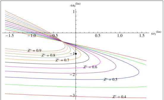
We begin with the model where the EEoS is linear in redshift, w(lin)₍_Z₎_{. In Fig.}

3.1 are shown w₀(lin) −w(lin)₁ curves for Z∗ in the range 0.4 ≤ Z∗ ≤ 0.9. Several interesting features of Fig. 3.1 deserve discussion. First, the dot at (0, -1) confirms

Z∗ = 0.743 ±0.030 for the CC model. If Z∗ is measured to be Z∗ > 0.75, it is necessary thatw(lin)₁ <0. IfZ∗is meaured to beZ∗ >0.831, we find thatw₀(lin) >−1. AsZ∗ increases, the requisite w(lin)₍_Z₎ _{becomes more and more distinct from the}

CC model. In Fig. 3.1, we note that for any measured value ofZ∗, there are two

possible values ofw(lin)₀ for each value ofw₁(lin).

(39)

Z* =0.4 Z*

=0.5 Z*

=0.6 Z*

=0.7 Z*

=0.8 Z*

=0.9

-1.5 -1.0 -0.5 0.5 1.0 1.5

Ω1H linL

-3 -2 -1 1 Ω0H

linL

Figure 3.1: w(lin)₀ is plotted against w₁(lin)for0.4 ≤ Z∗ ≤ 0.9 in increments of0.05. The dot at (0,-1) represents the CC model. Here we useΩm(t0) = 0.275, which is consistent with the result of

[48] for the best fit for this model.

The reader will remark the confluence of theZ∗-orbits in Fig. 3.1, which is an

artifact of the restriction to0.4≤Z∗ ≤0.9. For values ofZ∗near to but outside this range, the confluence desists. A similar phenomenon appears in later plots.

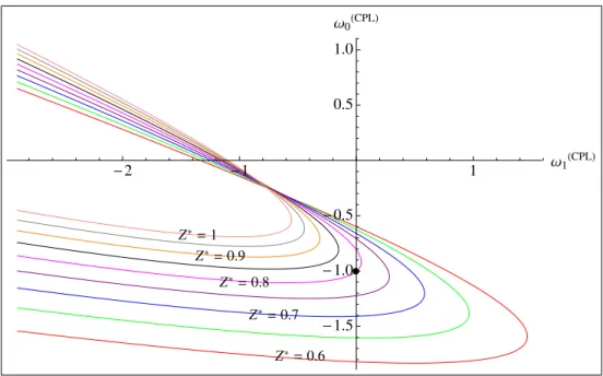
We next discuss the model w(CP L)(Z) [45, 46] in which the EEoS is linear in (1−a), whereais the scale factor. In Fig. 3.2 are shownw₀(CP L)−w(CP L)₁ curves for

Z∗ in the range0.6 ≤ Z∗ ≤ 1.0. There are several features of Fig. 3.2 to note. The dot at (0, -1) confirmsZ∗ = 0.8, which is the resultingZ∗value from Eq.(3.5) when

the valueΩm(t0) = 0.255is used, as determined by [47] as the best fit value for the

CPL model. If Z∗ is measured to beZ∗ > 0.810, we find thatw(CP L)₁ < 0. As Z∗

increases, the necessaryw(CP L)(Z) becomes more and more distinct from the CC model. In Fig. 3.2, we see that for any measured value ofZ∗, there are two possible

values ofw(CP L)₀ for each value ofw₁(CP L).

Now we examine Fig. 3.3 for the SSS model. We see that for a certain range

of Z∗ > 0.8, which includes the best fit value of Z∗ which we discuss later, both

(40)

Z* =0.6 Z* =0.7 Z* =0.8 Z* =0.9 Z* =1

-2 -1 1

Ω1H CPLL -1.5 -1.0 -0.5 0.5 1.0 Ω0H

CPLL

Figure 3.2: w(CP L)₀ is plotted againstw(CP L)₁ for0.6 ≤Z∗ ≤ 1.0in increments of0.05. The dot at (0,-1) represents the CC model. We useΩm(t0) = 0.255, which is consistent with the analysis in

[47] for the best fit for this model.

Z* =0.8 Z* =0.6 Z* =0.7 Z* =0.9 Z* =0.85 Z* =0.6 Z*₌_0.7

Z* =0.8 Z*

=0.9

-5 5 Ω1

HSSSL

-1.0 -0.5 0.5 1.0 1.5 Ω0H

SSSL

Figure 3.3: w₀(SSS) is plotted againstw(SSS)₁ for0.6 ≤ Z∗ ≤ 0.9in increments of0.05. We use

(41)

Z* =0.6 Z*

=0.7 Z*

=0.8 Z*

=0.9

-1.5 -1.0 -0.5 0.5 1.0 1.5

Ω1H newL

-1.5 -1.0 -0.5 Ω0H

newL

Figure 3.4: w(new)₀ is plotted againstw(new)₁ for0.6≤Z∗ _≤₀_.₉_{in increments of}₀_.₀₅_{. The dot at}

(0,-1) represents the CC model. We useΩm(t0) = 0.275.

w(SSS)₁ andw(SSS)₀ must be greater than zero. Note also the degeneracy inw(SSS)₀ for

Z∗ = 0.85,0.9.

Fig. 3.4 displays the new model. Once again we see that the CC model has

Z∗ = 0.743. ForZ∗ ≥ 0.81,w(new)₀ >−1.0. We note that forZ∗ >0.75,w(new)₁ must be negative.

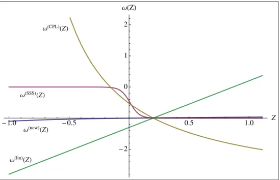
In Fig. 3.5, we show w(lin)₍_Z₎_, _w(CP L)₍_Z₎_{, and} _w(SSS)₍_Z₎ _{as a function of} _Z

(including the future,−1≤Z <0) using the best-fit parameters of [48] forw(lin)₍_Z₎

and those of [47] for the other 2 models. w(new)₍_Z₎_{is also plotted using the choice}

ofw(new)₀ =−1andw₁(new)= 0.1.

Unlike the CC model, where the future of the universe is infinite exponential

expansion, the best fit for w(lin)(Z) necessarily leads to a big rip, at a finite time in the future. The EEoS for w(CP L)₍_Z₎ _{possesses singular behavior for} _Z _{→ −}₁

because w(CP L)₍_Z₎ _{→ ±∞}_for_w(CP L)

1 being negative or positive, respectively. For

the SSS model,w(SSS)₍_Z₎_{varies in the range}₀_{> w}(SSS)₍_Z₎_>₋₁_.

(42)

ΩHCPLLHZL

ΩHSSSLH_ZL

ΩHnewLHZL

ΩHlinLH_ZL

-1.0 -0.5 0.5 1.0 Z

-2

0 1 2

ΩHZL

Figure 3.5: w(Z)for all the models is plotted againstZ from the highestZ∗ value toZ = −1

(when the scale factorais infinite). The horizontal axis atw(Z) = −1is the line representing the CC model. We usew₀(lin) = −1.3,w(lin)₁ = 1.5, andZ∗ = 0.4067(from the best fit for this model given in [48]). We usew₀(CP L)=−0.522,w₁(CP L)=−2.835, andZ∗ = 1.11for the CPL model and

(43)

As for our fourth and last model w(new)₍_Z₎_{, from Eq.(3.9), we note that this}

choice has the advantage that for allZthis EEoS lies between(w(new)₀ −w₁(new))and

(w₀(new)+w₁(new)). This is illustrated in Fig 3.5 where, for the choicesw₀(new) = −1.0 andw₁(new)= +0.1, the EEoS falls smoothly from−0.9at the big bang to−1.1at the big rip.

3.4 Slowly Varying Criteria

We now discuss which w(Z)for dark energy is the best for observers to employ.

Regretfully, there is no theoretical guidance about evolution. Nevertheless, we

here propose slowly varying criteria which is based purely on grounds of

aesthet-ics and, especially, conservatism. All the present data are consistent with the CC

modelw(CC) _{≡ −}_{1. We choose to remain proximate to it, as supported by [49, 50].}

One consideration is that we prefer any globalw(Z)to have analytic, non-singular

behavior forZ → −1 and Z → ∞. Finally, we propose to impose the inequality representing conservatism,

|w(Z) + 1| 1 for all −1≤Z <∞. (3.10)

Next, we consider application of our slow variation criteria to the four specific

models we have discussed in tbe present article. For this task, Fig. 3.5 will be used.

To be fair to their inventors, these EEoS were intended to apply for only a limited

range of redshift.

(i) Linear model

By studying the EEoS in Eq. (3.6), we notice that forZ →+∞,w(lin)(Z)approaches

±∞ depending on the sign of w₁(lin). Also, w(lin)(Z) violates the criterion of Eq.

(44)

(3.10). We conclude that this linear model is disfavored according to our slow

variation criteria.

(ii) CPL model

By examining the EEoS in Eq. (3.7), we note that asZ → −1, w(CP L)₍_Z₎_{→ ∓∞}_for

a (±) sign forw₁(CP L). Therefore, according to our criteria, this model is disfavored.

(iii) SSS model

Looking at Eq. (3.8), we see thatw(SSS)(Z)varies from0to−1for the best fit given in [47], so it is non-singular. By this token, however, it does not satisfy Eq. (3.10).

This model, then, is also disfavored by our criteria. It should be noted, though,

that [47] studied this EEoS as a toy model to illustrate the importance of an EEoS

that fits data well for small and large positiveZ.

(iv) New model

This model is non-singular for all−1≤Z <∞because [Z/(2+Z)] varies smoothly from−1to+1, as can be seen from examining Eq. (3.9). It also satisfies Eq. (3.10) if we choose appropriate values forw₀(new)andw₀(new).

3.5 Discussion and Conclusions

The outstanding observational question about dark energy is whether it is a CC

model with w(Z) ≡ −1 or an evolutionary model with a non-trivial EEoS. The model-independent observational measurement of Z∗ is very useful for making

this distinction.

The theoretical prediction of Z∗ is, however, dependent on the EoS that is

(45)

isZ∗ = 0.743±0.030. As the data become even more precise, the error onZ∗ will diminish, making it observationally easier to detect deviation, if any, from the CC

model.

In the four EEoS models listed earlier, the possible values of Z∗ for different

values of the parameters w0 and w1 can be read off from our plots. These plots

show that degeneracies appear. For a givenZ∗and a specific type of EEoS, there is

an allowed curve in thew1-w0plane. For all0.4≤Z∗ ≤1.0, there exist disallowed

regions in thew1-w0plane.

To go further, we have to give criteria for selecting one EEoS. The most popular

choice in the last few years has been the CPL model [45, 46] because it

approxi-mates the linear model at low redshift. Also, it has a simple interpretation in terms

of the scale factor:

w(CP L)(Z) =w(CP L)₀ +w₁(CP L)(1−a(Z)) (3.11)

However, as a(Z) → ∞ (Z → −1), the CPL model diverges. Of course, the authors of [45, 46] intended their model to be applicable only for a limited range

of Z. However, it seems preferable for w(Z) to cover the entire range of cosmic

history, both the past and future.

Our novel EEoS also approximates the linear model at low redshift. It has,

like the CPL model, a straightforward physical interpretation in terms of the scale

factor:

w(new)(Z) =w(new)₀ +w₁(new)

1−a(Z) 1 +a(Z)

(3.12)

We think one advantage of this new model over the CPL model is that it is

non-singular for−1 ≤ Z < ∞. A second advantage is that it can satisfy the slow variation criterion of Eq. (3.10).

(46)

In conclusion, the choice of an evolutionary alternative to the CC model

de-pends theoretically on constraining the EEoS, and we have proposed a new EEoS

which not only has a simple physical interpretation but also is well-behaved for

all possible redshifts. The model-independent extraction ofZ∗ from observational

data is a familiar process [51]. A more accurate model-independent estimate ofZ∗

by global fits to all relevant data is worthwhile. It is an interesting issue how the

present considerations of evolutionary dark energy are related to the possible

oc-currence of a big rip. This requires ultra-negative pressures of dark energy, so it is

interesting that situations involving phantom energy have appeared in the context

of extra spatial dimensions in string theory [52].

It has been argued [53] that dark energy effects can be detected only by

study-ing physical systems as large as galaxies. Thus, it is unlikely that any terrestrial

experiment can be sensitive to dark energy.

Understanding dark energy may, or may not (in the CC model), require a

grav-itational theory more complete than general relativity, which has been accurately

confirmed [54] only at the scale of the solar system, say∼1012meters, while dark energy operates above the galactic size, say∼ 1020meters. Thus, it is likely, even probable, that study of dark energy will inform us, in the near future, how to go

beyond Einstein, which is the most important direction both for particle physics

(47)

Chapter 4 The Little Rip

1

4.1 Introduction

Observations indicate that roughly 70% of the energy density in the universe is in

the form of an exotic, negative-pressure component, dubbed dark energy [56, 57].

(See Ref. [58] for a recent review.) If ρDE and pDE are the density and pressure,

respectively, of the dark energy, then the dark energy can be characterized by the

equation-of-state parameterwDE, defined by

wDE =pDE/ρDE. (4.1)

It was first noted by Caldwell [28] that observational data do not rule out the

possibility thatwDE <−1. Such “phantom” dark energy models have several

pe-culiar properties. The density of the dark energy increases with increasing scale factor, and both the scale factor and the phantom energy density can become

infi-nite at a fiinfi-nitet, a condition known as the “big rip” [28, 29, 59, 60]. It has even been

suggested that the finite lifetime for the universe in these models may provide an

6263.pdf

Modeling Dark Matter and Dark Energy

Abstract

Acknowledgments

Table of Contents

List of Figures

List of Tables

Chapter 1

Introduction

1.1

Historical Background

1.2

Overview of Dark Matter and Dark Energy

1.3

Motivation and Plan of this Work

Chapter 2

Number and Entropy of Black Holes

1

2.1

Introduction

2.2

Number of Black Holes

2.3

Entropy of Black Holes

2.4

Reconsideration of the Entropy of the Universe

Chapter 3

Seeking Evolution of Dark Energy

1

3.1

Introduction

3.2

Evolutionary Dark Energy Models

3.3

Analysis of the Models

3.4

Slowly Varying Criteria

3.5

Discussion and Conclusions

Chapter 4

The Little Rip

1

4.1

Introduction