Competing in the Dark: An Efficient Algorithm for Bandit Linear Optimization
Jacob Abernethy Computer Science Division
UC Berkeley [email protected]
Elad Hazan IBM Almaden [email protected]
Alexander Rakhlin Computer Science Division
UC Berkeley
Abstract
We introduce anefficientalgorithm for the prob-lem of online linear optimization in the bandit set-ting which achieves the optimal O∗(√T) regret. The setting is a natural generalization of the non-stochastic multi-armed bandit problem, and the ex-istence of an efficient optimal algorithm has been posed as an open problem in a number of recent papers. We show how the difficulties encountered by previous approaches are overcome by the use of a self-concordant potential function. Our approach presents a novel connection between online learn-ing and interior point methods.
1
Introduction
One’s ability to learn and make decisions rests heavily on the availability of feedback. Indeed, an agent may only improve itself when it can reflect on the outcomes of its own taken actions. In many environments feedback is readily available: a gambler, for example, can observe entirely the outcome of a horse race regardless of where he placed his bet. But such perspective is not always available in hindsight. When the same gambler chooses his route to travel to the race track, perhaps at a busy hour, he will likely never learn the outcome of possible alternatives. When betting on horses, the gambler has thus the benefit (or perhaps the detriment) to muse “I should have done...”, yet when betting on traffic he can only think“the result was...”.
This problem of sequential decision making was stated by Robbins [18] in 1952 and was later termed “the multi-armed bandit problem”. The name inherits from the model whereby, on each of a sequence of rounds, a gambler must pull the arm on one of several slot machines (“one-armed bandits”) that each returns a reward chosen stochastically from a fixed distribution. Of course, an ideal strategy would simply be to pull the arm of the machine with the greatest re-wards. However, as the gambler does not know the best arm a priori, his goal is then to maximize the reward of his strat-egy relative to reward he would receive had he known the optimal arm. This problem has gained much interest over the past 20 years in a number of fields, as it presents a very natural model of an agent seeking to simultaneously explore the world while exploiting high-reward actions.
As early as 1990 [8, 13] the sequential decision problem was studied under adversarial assumptions, where we as-sume the environment may even try to hurt the learner. The multi-armed bandit problem was brought into the adversar-ial learning model in 2002 by Auer et al [1], who showed that one may obtain nontrivial guarantees on the gambler’s performance relative to the best armeven when the arm val-ues are chosen by an adversary! In particular, Auer et al [1] showed that the gambler’sregret, i.e. the difference between the gain of the best arm minus the gain of the gambler, can be bounded byO(√N T)whereN is the number of bandit arms, andTis the length of the game. In comparison, for the game where the gambler is given full information about al-ternative arms (such as the horse racing example mentioned above), it is possible to obtainO(√TlogN), which scales better inNbut identically inT.
One natural and well studied problem, which escapes the Auer et al result, is that of “online shortest path”, considered in [11, 20] among others. In this problem the decision set is exponentially large (i.e., the set of all paths in a given graph), and the straightforward reduction of modeling each path as an arm for the multi-armed bandit problem suffers from both efficiency issues as well as regret exponential in the descrip-tion length of the graph. To cope with these issues, several authors [2, 9, 14] have recently proposed a very natural gen-eralization of the multi-armed bandit problem to the field of Convex Optimization, and we will call this “bandit linear op-timization”. In this setting we imagine that, on each round t, an adversary chooses some linear functionft(·)which is
not revealed to the player. The player then chooses a pointxt
within some given convex set1K ⊂
Rn. The player then suf-fersft(xt)and this quantity is revealed to him. This process
continues forTrounds, and at the end the learner’s payoff is hisregret:
RT = T
X
t=1
ft(xt)− min
x∗∈K
T
X
t=1
ft(x∗).
Online linear optimization has been often considered, yet primarily in the full-information setting where the learner sees all offt(·)rather than justft(xt). In the full-information
model, it has been known for some time that the optimal re-gret bound isO(√T), and it had been conjectured that the
1
In the case of online shortest path, the convex set can be rep-resented as a set of vectors inR|E|. Hence, the dependence on number of paths in the graph can be circumvented.
same should hold for the bandit setting as well. Neverthe-less, several initially proposed algorithms were shown only to obtain bounds with O(T3/4) (e.g. [14, 9]) orO(T2/3)
(e.g. [2, 7]). Only recently was this conjecture proven to be true by Dani et al. [6], who provided an algorithm with O(poly(n)√T) regret. However, their proposed method, which deploys a clever reduction to the multi-armed bandit algorithm of Auer et al [1], is not efficient.
We propose an algorithm for online linear bandit opti-mization that is the first, we believe, to be both computa-tionally efficient and achieve aO(poly(n)√T)regret bound. Moreover, with a thorough analysis we aim to shed light on the difficulties in obtaining such an algorithm. Our technique provides a curious link between the notion of Bregman diver-gences, which have often been used for constructing and an-alyzing online learning algorithms, and self-concordant bar-riers, which are of great importance in the study of interior point methods in convex optimization. A rather surprising consequence is that divergence functions, which are widely used as a regularization tool in online learning, provide the right perspective for the problem of managing uncertainty given limited feedback. To our knowledge, this is the first time such connections have been made.
2
Notation and Motivation
LetK ⊂Rnbe a compact closed convex set. For two vectors
x,y ∈ Rn, we denote their dot product asxTy. We write
ABif(A−B)is positive semi-definite. Let DR(x,y) :=R(x)− R(y)− ∇R(y)T(x−y) be theBregman divergencebetweenxandywith respect to a convex differentiableR.
Define the Minkowsky function (see page 34 of [16] for details) onK, parametrized by a poleytas
πyt(xt) = inf{t≥0 :yt+t−1(xt−yt)∈ K}.
We define a scaled version ofKby
Kδ ={u:πx1(u)≤(1 +δ)
−1 }
forδ >0. Herex1is a “center” ofKdefined in the later
sec-tions. We assume thatKis not “flat” and sox1is a constant distance away from the boundary.
In the rest of the section we describe the rich body of previous work which led to our result. The reader familiar with online optimization in the full and partial information settings can skip directly to the next section.
Theonline linear optimizationproblem is defined as the following repeated game between the learner (player) and the environment (adversary).
At each time stept= 1toT,
• Player choosesxt∈ K
• Adversary independently choosesft∈Rn
• Player suffers lossfT
txtand observes feedback=
The goal of the Player is not simply to minimize his to-tal lossPT
t=1f T
txt, for an adversary could simply chooseft
to be as large as possible at every point inK. Rather, the Player’s goal is to minimize hisregretRT defined as
RT := T
X
t=1 fT
txt− min
x∗∈K
T
X
t=1 fT
tx∗.
When the objective is his regret, the Player is not compet-ing against arbitrary strategies, he need only perform well relative to the total loss of the single best fixed point inK.
We distinguish thefull-information andbanditversions of the above problem. The full-information version, the Player may observe the entire functionftas his feedback=and can
exploit this in making his decisions. In this paper we study the more challenging bandit setting, where the feedback=
provided to the player on roundt is only the scalar value
fT
txt. This is significantly less information for the Player:
instead of observing the entire functionft, he may only
wit-ness the value offtat a single point.
2.1 Algorithms Based on Full Information
All previous work on bandit online learning, including the present one, relies heavily on techniques developed in the full-information setting and we now give a brief overview of some well-known approaches.
Follow The Leader (FTL) is perhaps the simplest online learning strategy one might think of: the player simply uses the heuristic “select the best choice thus far”. For the online optimization task we study, this can be written as
xt+1:= arg min
x∈K
t
X
s=1 fT
sx. (1)
For certain types of problems, applying FTL does guaran-tee low regret. Unfortunately, when the loss functionsftare
linear on the input space it can be shown that FTL will suf-fer regret that grows linearly inT. A natural approach2, and
more well-known within statistical learning, is toregularize
the optimization problem (1). That is, an appropriate reg-ularization function R(x) and a trade-off parameterλ are selected, and the prediction is obtained as
xt+1:= arg min
x∈K
" t
X
s=1 fT
sx+λR(x)
#
. (2)
We call the above approach Follow The Regularized Leader (FTRL). An alternative way to view this exact algorithm is by sequential updates, which capture the difference between consecutive solutions for FTRL. Given thatRis convex and differentiable, the general form of this update is
¯
xt+1=∇R∗(∇R(¯xt)−ηft), (3)
followed by a projection ontoK with respect to the diver-genceDR:
xt+1= arg min
u∈KDR(u,x¯t+1).
HereR∗ is the Fenchel dual function andηis a parameter. This procedure is known as the mirror descent (e.g. [5]).
2
In the context of classification, this approach has been formu-lated and analyzed by Shalev-Shwartz and Singer [19].
Applying the above rule we see that the well known On-line Gradient Descent algorithm [21, 10] is derived3by
choos-ing the regularizer to be the squared Euclidean norm. Simi-larly, the Exponentiated Gradient [12] algorithm is obtained with the entropy function as the regularizer.
This unified view of various well-known algorithms as solutions to regularization problems gives us an important degree of freedom of choosing the regularizer. Indeed, we will choose a regularizer for our problem that possesses key properties needed for the regret to scale asO(√T). In Sec-tion 4, we give a bound on the regret for (2) with any regular-izerRand in Section 5 we will discuss the specificRused in this paper.
2.2 The Dilemma of Bandit Optimization
Effectively all previous algorithms for the Bandit setting have utilized a reduction to the full-information setting in one way or another. This is reasonable: any algorithm that aimed for low-regret in the bandit setting would necessarily have to achieve low regret given full information. Furthermore, as the full-information online learning setting is relatively well-understood, it is natural to exploit such techniques for this more challenging problem.
The crucial reduction that has been utilized by several au-thors [1, 2, 6, 7, 14] is the following. First choose some full-information online learning algorithmA.Awill receive in-put vectorsf1, . . . ,ft, corresponding to previously observed
functions, and will return some pointxt+1 ∈ K to predict.
On every roundt, do oneor bothof the following:
• QueryAfor its predictionxtand either predictxt
ex-actly or in expectation.
• Construct some random estimate˜ftin such a way that
E˜ft = ft, and input˜ft into A as though it had been
observed on this round
The key idea here is simple: so long as we are roughly pre-dictingxtper advice of A, and so long as we are
“guess-ing”ft(i.e. so that the estimates˜ftis correct in expectation),
then we can guarantee low regret. This approach is validated in Lemma 3 which shows that, as long asAperforms well against the random estimates˜ftin expectation, then we will
also do well against the true functionsf1, . . . ,fT.
This observation is quite reassuring yet unfortunately does not address a significant obstacle: how can we simultane-ously estimate˜ftand predictxtwhen only one query is
al-lowed?The algorithm faces an inherent dilemma: whether to follow the advice ofAof predictingxt, or to try to estimate
ft by sampling in a wide region around K, possibly
hurt-ing its performance on the given round. This exploration-exploitation trade-off is the primary source of difficulty in obtainingO(√T)guarantees on the regret.
Roughly two categories of approaches have been sug-gested to perform both exploration and exploitation:
1. Alternating Explore/Exploit:Flip an-biased coin to determine whether to explore or exploit. On explore 3
Strictly speaking, this equivalence is true if the updates are ap-plied to unprojected versions ofxt.
rounds, sample uniformly on some wide region around
Kand estimateftaccordingly, and input this intoA. On
exploit rounds, queryAforxtand predict this.
2. Simultaneous Explore/Exploit: QueryA for xtand
construct a random vector Xt such that EXt = xt.
Construct˜ftrandomly based on the outcome ofXtand
the learned valuefT
tXt.
The methods of [14, 2, 7] fit within in the first category but, unfortunately, fail to obtain the desiredO(poly(n)√T) re-gret. This is not surprising: it has been suggested by [7] that Ω(T2/3)regret is unavoidable by any algorithm in which the
observationfT
txtis ignored on rounds pledged for
exploita-tion. Algorithms falling into the second category, such as those of [1, 6, 9], are more sophisticated and help to moti-vate our results. We review these methods below.
2.3 Methods For Simultaneous Exploration and Exploition
On first glance, it is rather surprising that one can perform the task of predicting somext(in expectation) while,
simul-taneously, finding an unbiased estimate offt. To get a feel
for how this can be done, we briefly review the methods of [1] and [9] below.
The work ofAuer et al [1]is not, strictly speaking, con-cerned with a general bandit optimization problem but in-stead the more simple “Multi-armed bandit” problem. The authors consider the problem of sequentially choosing one ofN“arms” each of which contains a hidden loss where the learner may only see the loss of his chosen arm. The regret, in this case, is the learner’s loss minus the smallest cumula-tive loss over all arms. This multi-armed bandit problem can indeed be cast as a bandit optimization problem: letKbe the N-simplex (convex hull of{e1, . . . ,eN}), let ft be
identi-cally the vector of hidden losses on the set of arms, and note thatminx∈KPfsTx= miniPfs[i].
The algorithm of [1], EXP3, utilizes EG (mentioned ear-lier) as its black box full-information algorithmA. First, a pointxt ∈ Kis returned byA. The hypothesisxtis then
biasedslightly:
xt←(1−γ)xt+γ
1 n, . . . ,
1 n
.
We describe the need for this bias in Section 2.4. EXP3 then randomly chooses one of the corners ofKaccording to the distributionxtand uses this as its prediction. More precisely,
a basis vectoreiis sampled with probabilityxt[i]and clearly
EI∼xteI =xt. Once we observef T
tei =ft[i], the estimate
is constructed as follows:
˜ft:=
f
t[i]
xt[i]
ei.
It is very easy to check thatE˜ft=ft.
Flaxman et al [9]developed a bandit optimization algo-rithm that used OGD as the full-information subroutineA. Their approach uses a quite different method of performing exploration and exploitation. On each round, the algorithm queriesAfor a hypothesisxtand, as in [1], this hypothesis
is biased slightly:
whereuis some “center” vector of the setK. Similarly to EXP3, the algorithm doesn’t actually predict xt. The
al-gorithm determines the distance r to the boundary of the set, and a vectorrv is sampled uniformly at random from a sphere of radiusr. The prediction isyt := xt+rv and
indeedEyt=xt+rEv=xtas desired. The algorithm
pre-dictsyt, receives feedbackftTyt, and functionftis estimated
as
˜ft:= ftTyt
r v.
It is, again, easy to check that this provides an unbiased esti-mate offt.
2.4 The Curse of High Variance and the Blessing of Regularization
Upon inspecting the definitions of˜ftin the method of Auer
et al and Flaxman et al it becomes apparent that the estimates are inversely proportional to the distance ofxtto the
bound-ary. This implies high variance of the estimated functions. At first glance, this seems to be a disaster. Indeed, most full-information algorithms scale linearly with the magnitude of the functions played by the environment. Let us take a closer look at how exactly this leads to the suboptimality of the al-gorithm of Flaxman et al.
The bound on the expected regret of OGD on˜ft’s
in-volves termsEk˜ftk2(see proof of Lemma 2), which scale as
the inverse of the squared distance to the boundary. Biasing ofxtaway from the boundary leads to an upper bound on this
quantity of the orderγ−2. Unfortunately,γcannot be taken to be large. Indeed, the optimal point x∗, chosen in hind-sight, lies on the boundary of the set, as the cost functions are linear. Thus, stepping away from the boundary comes at a cost of potentially losingO(γT)over the course of the game. Since the goal is to obtain anO(√T)bound on the regret,γ=O(T−1/2)is the most that can be tolerated.
Bi-asing away from the boundary does reduce the variance of the estimates somewhat; unfortunately, it is not the panacea. To terminate the discussion on the method of Flaxman et al, we state the dependence of the regret bound on the learning rateηand the biasing parameterγ:
RT =O(η−1+γ−2ηT+γT).
The first term is due to the distance between the initial choice and the comparator; the second is the problematic Ek˜ftk2
term summed over time; and the last term is due to stepping away from the boundary. The best choice of the parameters leads to the unsatisfyingO(T3/4)bound.
From the above discussion it is clear that the problematic term isEk˜ftk2 =O(1/r2), owing its high magnitude to its
inverse dependence on the squared distance to the boundary. A similar dependence occurs in the estimate of Auer et al, though the non-uniform sampling from the basis implies an O(1/xt[i])magnitude. One can ask whether this inverse
de-pendence on the distance is an artifact of these algorithms and can be avoided. In fact, it is possible to prove that this is intrinsic to the problem if we require that˜ftbe unbiased and
xtbe the center of the sampling distribution.
Does this result imply that noO(√T)bound on the re-gret is possible? Fortunately, no. If we restrict our search
to a regularization algorithm of the type (2), the expected regret can be proved to beequalto an expression involving EDR(xt,xt+1)terms. ForR(x)∝ kxk2we indeed recover
(modulo projections) the method of Flaxman et al with its in-surmountable hurdle ofEk˜ftk2. Fortunately, other choices of
Rhave better behavior. Here, the formulation of the regular-ized minimization (2) as a dual-space mirror descent comes to the rescue.
In the space of gradients (the dual space), the step-wise updates (3) for Follow The Regularized Leader areη˜ft no
matter whatRwe choose. It is a known fact (e.g. [5]) that the divergence in the original space betweenxtandxt+1is
equal to the divergence between the corresponding gradients with respect to the dual potential R∗. It is, therefore, not surprising that the dual divergence can be tuned to be small even ifk˜ftk is very large. Having small divergence
corre-sponds to the requirement thatR∗be “flat” wheneverk˜ftkis
large, i.e. whenxtis close to the boundary. Flatness in the
dual space corresponds to large curvature in the primal. This motivates the use of a potential functionRwhich becomes more and more curved at the boundary of the setK. In a nut-shell, this is the Blessing of Regularization which allows us to obtain an efficient optimal algorithm which was escaping all previous attempts.
Recall that the method of Auer et al attains the optimal O(√T)rate but only when K is the simplex. If our intu-ition about the importance of regularization is sound, we should find that the method uses a potential which curves at the edges of the simplex. One can see that the exponen-tial weights (more generally, EG) used by Auer et al corre-sponds to regularization withRbeing the entropy function
R(x) = Pn
i=1x[i] logx[i]. Taking the second derivative,
we see that, indeed, the curvature increases as1/x[i]as x
gets closer to the boundary. For the present paper, we will actually choose a regularizer that curves as inversesquared
distance to the boundary. The reader can probably guess that such a regularizer should be defined, roughly, as the log -distance to the boundary.
While for simple convex bodies, such as sphere, exis-tence of a function behaving likelog-distance to the bound-ary seems plausible, a similar statement for general convex setsKseems very complex. Luckily, this very question has been studied in the theory of Interior Point Methods, and ex-istence and construction of such functions, calledself- con-cordant barriers, is well-established.
3
Main Result
We first state our main result: an algorithm for online linear optimization in the bandit setting for an arbitrary compact convex setK. The analysis of this algorithm has a number of facets and we discuss these individually throughout the re-mainder of this paper. In Section 4 we describe the regular-ization framework in detail and show how the regret can be computed in terms of Bregman divergences. In Section 5 we review the theory of self-concordant functions and state two important properties of such functions. In Section 6 we high-light several key elements of the proof of our regret bound. In Section 7 we show how this algorithm can be used for one interesting case, namely the bandit version of the Online
Algorithm 1Bandit Online Linear Optimization
1: Input:η >0,ϑ-self-concordantR
2: Letx1= arg minx∈K[R(x)].
3: fort= 1toTdo
4: Let {e1, . . . ,en} and {λ1, . . . , λn} be the set of
eigenvectors and eigenvalues of∇2R(x
t).
5: Chooseituniformly at random from{1, . . . , n} and
εt=±1with probability1/2.
6: Predictyt=xt+εtλ−
1/2
it eit.
7: Observe the gainfT
tyt∈R.
8: Define˜ft:=n(ftTyt)εtλ
1/2
it ·eit.
9: Update
xt+1= arg min
x∈K
"
η
t
X
s=1 ˜ fT
sx+R(x)
#
.
10: end for
Shortest Path problem. The precise analysis of our algorithm is given in Section 8. Finally, in Section 9 we spell out how to implement the algorithm with only one iteration of the Damped Newton method per time step.
The following theorem is the main result of this paper (see Section 5 for the definition ofϑ-self-concordant barrier). Theorem 1 LetKbe a convex set andRbe aϑ-self-concordant barrier onK. Letube any vector inK0=K
1/√T. Suppose
we have the property that|fT
tx| ≤1for anyx∈ K. Setting
η= √
ϑlogT
4n√T , the regret of Algorithm 1 is bounded as
E
T
X
t=1 fT
tyt≤ min
u∈K0E
T
X
t=1 fT
tu
!
+ 16npϑTlogT
wheneverT >8ϑlogT.
The expected regret over the original setKis within an additiveO(√nT)factor from the above guarantee, as im-plied by Lemma 8 in the Appendix.
4
Regularization Algorithms and Bregman
Divergences
As our algorithm is clearly based on a regularization frame-work, we now state a general result for the performance of any algorithm minimizing the regularized empirical loss. We call this method Follow the Regularized Leader, and we de-fer the proof of the regret bound to the Appendix. A similar analysis for convex loss functions can be found in [5], Chap-ter 11. We remark that the use of Bregman divergences in the context of online learning goes back at least to Kivinen and Warmuth [12].
Let˜f1, . . . ,˜fT ∈ Rn be any sequence of vectors. Sup-posext+1is obtained as
xt+1= arg min
x∈K
"
η
t
X
s=1 ˜fT
sx+R(x)
#
| {z }
Φt(x)
(4)
for some strictly-convex differentiable functionR. We de-noteΦ0(x) =R(x)andΦt= Φt−1+η˜ft.
We will assume∇Rapproaches infinity at the boundary of K so that the unconstrained minimization problem will have a unique solution within K. We have the following bound on the performance of such an algorithm.
Lemma 2 For anyu∈ K, the algorithm defined by(4) en-joys the following regret guarantee
η
T
X
t=1 ˜fT
t(xt−u) ≤ DR(u,x1) +
T
X
t=1
DR(xt,xt+1)
≤ DR(u,x1) +η
T
X
t=1 ˜fT
t(xt−xt+1) for any sequence{˜ft}Tt=1.
In addition, we state a useful result that bounds the true regret based on the regret against the estimated functions˜ft.
Lemma 3 Suppose that, for t = 1, . . . , T,˜ftis such that
E˜ft = ftand ytis such thatEyt = xt. Suppose that we
have the following regret bound:
T
X
t=1 ˜fT
txt≤min
u∈K0
T
X
t=1 ˜fT
tu+CT.
Then the expected regret satisfies
E
T
X
t=1 fT
tyt
!
≤min u∈K0E
T
X
t=1 fT
tu
!
+CT.
5
Self-concordant Functions and the Dikin
ellipsoid
Interior-point methods are arguably one of the greatest achieve-ments in the field of Convex Optimization in the past two decades. These iterative polynomial-time algorithms for Con-vex Optimization find the solution by adding a barrier func-tion to the objective and solving the unconstrained minimiza-tion problem. The rough idea is to gradually reduce the weight of the barrier function as one approaches the solu-tion. The construction of barrier functions for general convex sets has been studied extensively, and we refer the reader to [16, 4] for a thorough treatment on the subject. To be more precise, most of the results of this section can be found in [15], page 22-23, as well as in the aforementioned texts. 5.1 Definitions and Properties
Definition 4 Aself-concordant functionR:intK →Ris a
C3convex function such that
|D3R(x)[h,h,h]| ≤2 D2R(x)[h,h]3/2.
Here, the third-order differential is defined as D3R(x)[h1,h2,h3] :=
∂3
∂t1∂t2∂t3
We will further assume that the function approaches infin-ity for any sequence of points approaching the boundary of
K. An additional requirement leads to the notion of a self-concordantbarrier.
Definition 5 Aϑ-self-concordant barrierRis a self-concordant function with
|DR(x)[h]| ≤ϑ1/2D2R(x)[h,h]1/2.
The generality of interior-point methods comes from the fact that any arbitraryn-dimensional closed convex set admits an O(n)-self-concordant barrier [16]. Hence, throughout this paper,ϑ=O(n), but can even be independent of the dimen-sion, as for the sphere.
We note that some of the results of this paper, such as the Dikin ellipsoid, rely onRbeing a self-concordant function, while others necessarily require the barrier property. We therefore assume from the outset thatRis a self-concordant barrier.
SinceKis compact, we can assume thatRis non-degenerate. For a givenx∈ K, define
hg,hix=gT∇2R(x)h and khkx= (hh,hix)−1/2. This inner product defines the local Euclidean structure atx. Nondegeneracy ofRimplies that the above norm is indeed a norm, not a seminorm.
It is natural to talk about a ball with respect to the above norm. Define the openDikin ellipsoidof radiusrcentered at
xas the set
Wr(x) ={y∈ K:ky−xkx< r}.
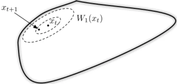
The following facts about the Dikin ellipsoid are central to the results of this paper (we refer to [15], page 23 for proofs). The first non-trivial fact is thatW1(x)⊆ Kfor anyx∈ K.
In other words, the inverse Hessian of the self-concordant functionRstretches the space in such a way that the eigen-vectors fall in the setK. This is crucial for our sampling pro-cedure. Indeed, our method (Algorithm 1) samplesytfrom
the Dikin ellipsoid centered atxt. SinceW1(xt)is contained
inK, the sampling procedure is legal.
The second fact is that within the Dikin ellipsoid, that is forkhkx <1, the Hessians ofRare “almost proportional” to the Hessian ofRat the center of the ellipsoid :
(1− khkx)2∇2R(x) ∇2R(x+h) (5)
(1− khkx)−2∇2R(x). This gives us the crucial control of the Hessians for second-order approximations. Finally, ifkhkx <1(i.e.x+his in the unit Dikin ellipsoid), then for anyz,
|zT(∇R(x+h)− ∇R(x))| ≤ khkx
1− khkx
kzkx. (6) Assuming thatRis aϑ-self-concordant barrier, we have (see page 34 of [16])
R(u)− R(x1)≤ϑln 1 1−πx1(u). For anyu∈ Kδ,πx1(u)≤(1+δ)
−1by definition, implying
that(1−πx1(u))
−1≤ 1+δ
δ . We conclude that
R(u)− R(x1)≤ϑln(√T+ 1)≤2ϑlogT (7) foru∈ K1/√
T.
5.2 Examples of Self-Concordant Functions
A nice fact about self-concordant barriers is thatR1+R2
isϑ1 +ϑ2-self-concordant forϑ1-self-concordantR1 and
ϑ2-self-concordantR2. For linear constraintsaTxt≤b, the
barrier−ln(b−aTx
t) is 1-self-concordant. Hence, for a
polyhedron defined bymconstraints, the corresponding bar-rier ism-self-concordant. Thus, for then-dimensional sim-plex or a cube,θ = n, leading ton3/2 dependence on the
dimension in the main result. For then-dimensional ball,
Bn ={x∈Rn,
X
i
x2i ≤1},
the barrier functionR(x) =−log(1−kxk2)is1-self-concordant.
This, somewhat surprisingly, leads to the linear dependence of the regret bound on the dimensionn, asϑ= 1.
6
Sketch of Proof
We have now presented all necessary tools to prove Theo-rem 1: regret in terms of Bregman divergences, self-concordant barriers and the Dikin ellipsoid. While we provide a com-plete proof in Section 8 here we sketch the key elements of the analysis of our algorithm.
As we tried to motivate in the end of Section 2, any method that can simultaneously (a) predict xt in
expecta-tion and (b) obtain an unbiased one-sample estimate of˜ft
will necessarily suffer from high variance whenxtis close
to the boundary of the setK. As we have hinted previously, we would like our regularizerRto control the variance. Yet the problem is even more subtle than this: xtmay be close
to the boundary in one dimension while have plenty of space in another, which in turn suggests that˜ftneed only have high
variance in certain directions.
Quite amazingly, the self-concordant function Rgives us a handle on two key issues. The Dikin ellipsoid, de-fined in terms∇2R(x
t), gives us exactly a rough
approxi-mation to the available “space” aroundxt. At the same time,
∇2R(x
t)−1annihilates˜ftin exactly the directions in which
it is large. This is absolutely necessary for bounding the re-gret, as we discuss next.
Lemma 2 implies that regret scales with the cumulative divergence η−1P
tDR(xt,xt+1) and thus we must have
thatEDR(xt,xt+1) = O(η2)on average to obtain a regret
bound ofO(√T). Analyzing the divergence requires some care and so we provide only a rough sketch here (with more in Section 8). IfR were exactly quadratic then the diver-gence is
DR(xt,xt+1) :=η2˜ftT(∇
2R(x
t))−1˜ft. (8)
Even when Ris not quadratic, however, (8) still provides a decent approximation to the divergence and, given cer-tain regularity conditions on R, it is enough to bound the quadratic form˜fT
t(∇2R(xt))−1˜ft.
The precise interaction between the Dikin ellipsoid, the estimates˜ft, and the divergenceDR(xt,xt+1)is as follows.
Assume we are at the pointxt and we have computed the
unit eigenvectorse1, . . . ,en and corresponding eigenvalues
λ1, . . . , λnof∇2R(xt). Properties of self-concordant
withinKand thus, in particular, so are the pointsxt±λ
−1/2
i ei
for eachi. Assuming the pointyt:=xt+λ
−1/2
j ejwas
sam-pled and we received the valuefT
tyt, we then construct the
estimate
˜ft:=np
λj(ftTyt)ej.
Notice it is crucial that we scale bypλj, theinverse`2
dis-tance betweenxtand yt, to ensure thatft is unbiased.On
the other hand, we see that the divergence is approximately computed as
DR(xt,xt+1) ≈ η2˜ftT∇2R−1˜ft
= η2n2(fT
tyt)2λj(eTj∇
2R−1e
j)
= η2n2(fT
tyt)2.
As an interesting and important aside, a necessary re-quirement of the above analysis is that we construct our es-timates˜ftfrom the eigendirectionsej. To see this, imagine
that one eigenvalueλ1is very large, while another,λ2small.
This corresponds to a thin and long Dikin ellipsoid, which would occur near a flat boundary. Suppose that instead of eigen-directions, we sample at an angle between them. With the thin ellipsoid the sampled points are still close in`2
dis-tance, implying that˜ftwill be large in both eigen-directions.
However, the inverse Hessian will only annihilate one of these directions.
7
Application to the online shortest path
problem
Because of its appealing structure, the online shortest path problem is one of the best studied problems in online opti-mization. Takimoto and Warmuth [20], and later Kalai and Vempala [11], gave efficient algorithms for the full informa-tion setting. Awerbuch and Kleinberg [2] were the first to give an efficient algorithm withO(T2/3)regret in the partial information (bandit) setting. The recent work of Dani et al [6] implies aO(m3/2√T)-regret algorithm, wherem=|E|
is the number of edges in the graph.
Turning to Algorithm 1, we notice that wheneverKis de-fined by linear constraints,Ris defined in a straightforward way (see Section 5.2). As we show below, the online shortest path is an optimization problem on such a set, and we obtain an efficientO(m3/2√T)-regret algorithm.
Formally, thebandit shortest pathproblem is defined as the following repeated game:
Given a directed graphG= (V, E)and a source-sink pair s, t∈V, at each time stept= 1toT,
• Player chooses a pathpt∈ Ps,t, wherePs,t⊆ {E}|V|
is the set of alls, t-paths in the graph
• Adversary independently chooses weights on the edges of the graphft∈Rm
• Player suffers and observes loss, which is the weighted length of the chosen pathP
e∈ptft(e)
The problem is transformed into an instance of bandit linear optimization by associating each path with a vector
x ∈ {0,1}|E|, wherex(i)indicates the presence of theith edge. The loss is then defined through the dot productfTx.
Define the setK as the convex hull of the set of paths. It is well-known that this set is the set of flows in the graph and can be defined usingO(m)constraints: positivity con-straints and conservation of in-flow and out-flow for every vertex other than source/sink (which have unit out-flow and in-flow, respectively).
Theorem 1 implies that Algorithm 1 attainsO(m3/2√T)
regret for the bandit linear optimization problem over this setK. However, an astute reader would notice that with this definition ofK, the algorithm produces a flowyt ∈ K, not
necessarily a path, at each round. The loss suffered by the online player isfT
tyt and the game is specified differently
from the bandit shortest path.
However, it is easy to convert this flow algorithm into a randomized online shortest path algorithm: according to the standard flow decomposition theorem (see e.g. [17]), a given flow in the graph can be decomposed into a distribution over at mostm+ 1paths in polynomial time. Hence, given a flow
yt ∈ K, one can obtain an unbiased estimator forftTytby
choosing a path according to the distribution of the decom-position, and estimatingfT
tytby the length of this path. In
fact, we have the following general statement.
Proposition 1 Suppose that, having computedytin step(1)
of Algorithm 1, we predict a randomy¯t∈ Ksuch thatEy¯t=
yt, and in step (1)observe ftTy¯t . If we use this observed
value instead offT
tytin step(1), the expected regret of the
modified algorithm is the same as that of Algorithm 1.
The proposition implies that the modified algorithm at-tains low regret for games defined over discrete sets of pos-sible predictions for the player. This is achieved by working with theconvex hullof the discrete set while predicting in the original set. In particular, the modification allows us to predict a legal path while the algorithm works with the set of flows.
The proof of Proposition 1 is straightforward: following closely the proof of Theorem 1, we observe that the value
fT
tytis used in only two places. The first is in Equation (9),
where it is upper-bounded by1, and the second is in the proof of the fact that˜ftis unbiased.
8
Proof of the regret bound
8.1 UnbiasednessFirst, we show thatE˜ft=ft. Condition on the choiceitand
average over the choice ofεt:
Eεt˜ft=
1 2n
ft·(xt+λ
−1/2
it eit)
λ1it/2·eit −1
2n
ft·(xt−λ
−1/2
it eit)
λ1it/2·eit
=n(fT
teit)eit.
Hence,
E˜ft=n Eiteite T
it
ft=ft.
xt
xt+1
W1(xt)
Figure 1: The Dikin ellipsoidW1(xt)atxt. The next
mini-mum is guaranteed to lie in its scaled versionW4nη(xt).
8.2 Closeness of the next minimum
We now use the properties of the Dikin ellipsoids mentioned in the previous section.
Lemma 6 The next minimizerxt+1is “close” toxt:
xt+1∈W4nη(xt).
Proof: Recall that
xt+1= arg min
x∈KΦt(x) and xt= arg minx∈KΦt−1(x) whereΦt(x) =ηP
t
s=1˜ftTx+R(x).Since∇Φt−1(xt) = 0,
we conclude that∇Φt(xt) =η˜ft.
Consider any point inz∈W1
2(xt). It can be written as z = xt+αufor some vectorusuch thatkukxt = 1 and
α∈(−1 2,
1
2). Expanding,
Φt(z) = Φt(xt+αu)
= Φt(xt) +α∇Φt(xt)Tu+α2
1 2u
T∇2Φ
t(ξ)u
= Φt(xt) +αη˜ftTu+α
21
2u
T∇2Φ
t(ξ)u
for someξon the path betweenxtandxt+αu.
Let us check where the optimum of the RHS is obtained. Setting the derivative with respect toαto zero, we obtain
|α∗|= η|
˜fT
tu|
uT∇2Φ
t(ξ)u
= η|
˜fT
tu|
uT∇2R(ξ)u.
The fact thatξis on the linexttoxt+αuimplies thatkξ−
xtkxt ≤ kαukxt < 1
2. Hence, by Eq (5), ∇2R(ξ)(1− kξ−x
tkxt)
2∇2R(x
t)
1 4∇
2R(x
t).
ThusuT∇2R(ξ)u> 1
4kukxt = 1
4, and hence
α∗<4η|˜fT
tu|.
Recall that˜ft=n(ft·yt)εtλ
1/2
it ·eitand so˜f T
tuis
max-imized/minimized whenuis a unit (with respect tok · kxt)
vector in the direction ofeit, i.e. u=±λ
−1/2
it eit. We
con-clude that
|˜fT
tu| ≤n|ft·yt| ≤n (9)
and
|α∗|<4nη < 1 2
by our choice ofη andT. We conclude that the local op-timumarg minz∈W1
2
(xt)Φt(z) is strictly insideW4nη(xt),
and sinceΦtis convex, the global optimum is
xt+1= arg min
z∈KΦt(z)∈W4nη(xt).
8.3 Proof of Theorem 1
We are now ready to prove the regret bound for Algorithm 1. Sincext+1 ∈ W4nη(xt), we invoke Eq (6) atx = xtand
z=h=xt+1−xt:
|hT(∇R(x
t+1)− ∇R(xt))| ≤
khk2
xt
1− khkxt
. Observe thatxt+1∈W4nη(xt)implieskhkxt <4nη.
The proof of Lemma 2 (Equation (12) in the Appendix) reveals that
∇R(xt)− ∇R(xt+1) =η˜ft.
We have
˜fT
t(xt−xt+1) =η−1hT(∇R(xt+1)− ∇R(xt))
≤η−1 khk
2
xt
1− khkxt ≤ 16n
2η
1−4nη
≤32n2η. (10)
By Lemma 2, for anyu∈ K1/√
T T
X
t=1 ˜fT
t(xt−u)≤η−1DR(u,x1) +
T
X
t=1 ˜fT
t(xt−xt+1) ≤η−1DR(u,x1) + 32n2ηT
=η−1(R(u)− R(x1)) + 32n2ηT
≤1
η(2ϑlogT) + 32n
2ηT,
where the first equality follows since∇R(x1) = 0, by the
choice ofx1; the last inequality follows from Equation (7). Balancing withη =
√
ϑlogT
4n√T , we get T
X
t=1 ˜fT
t(xt−u)≤16n
p
ϑTlogT .
for anyuin the scaled setK0. Using Lemma 3, which we prove below, we obtain the statement of Theorem 1. 8.4 Expected Regret
Note that it is not˜fT
txtthat the algorithm should be incurring,
but ratherfT
tyt. However, it is easy to see that these are equal
Proof:[Lemma 3] LetEt[·] =E[·|i1, . . . , it−1, ε1, . . . , εt−1]
denote the conditional expectation. Note that Et˜ftTxt=ftTxt=EtftTyt.
Taking expectations on both sides of the bound for˜ft’s,
E
T
X
t=1 ˜ fT
txt≤Emin u∈K0
T
X
t=1 ˜fT
tu+CT
≤ min u∈K0E
T
X
t=1 ˜fT
tu
!
+CT
= min u∈K0E
T
X
t=1 fT
tu
!
+CT.
In the case of an oblivious adversary,
min u∈K0E
T
X
t=1 fT
tu
!
= min u∈K0
T
X
t=1 fT
tu.
However, if the adversary is not oblivious,ftdepends on the
random choices at time steps1, . . . , t−1. Of course, it is desirable to obtain a stronger bound on the regret
E
" T
X
t=1 fT
tyt−min
u∈K0
T
X
t=1 fT
tu
#
=O(
√
T),
which allows the optimaluto depend on the randomness of the player4. Obtaining guarantees for adaptive adversaries is another dimension of the bandit optimization problem and is beyond the scope of the present paper.
Auer et al [1] provide a clever modification of their EXP3 algorithm which leads to high-probability bounds on the re-gret, thus guaranteeing low regret against an adaptive ad-versary. The modification is based on the idea of adding confidence intervals to the losses. The same idea has been employed in the work of [3] (note that [3] is submitted con-currently with this paper) for the bandit optimization over arbitrary convex sets. While the work of [3] does succeed in obtaining a high-probability bound, the algorithm is based on the inefficient method of Dani et al [6], which is a reduction to the algorithm of Auer et al.
9
Efficient Implementation
In this section we describe how to efficiently implement Al-gorithm 1. Recall that in each iteration our alAl-gorithm re-quires the eigen-decomposition of the Hessian in order to derive the unbiased estimator, which takesO(n3)time. This
is coupled with a convex minimization problem in order to compute xt, which seems to be the most time consuming
operation in the entire algorithm.
The message of this section is that the computation ofxt
given the previous iteratext−1takes essentially onlyone
it-eration of the Damped Newton method. More precisely, instead of using xt as defined in Algorithm 1, it suffices
4
It is known that the optimal strategy for the adversary does not need any randomization beyond the player’s choices.
to maintain a sequence of points {zt}, such that zt is
ob-tained fromzt−1by only one iteration of the Damped
New-ton method. The sequence of points{zt} are shown to be
sufficiently close to{ˆxt}, which enjoy the same guarantee
as the sequence of{xt}defined by Algorithm 1.
A single iteration of the Damped Newton method re-quires matrix inversion. However, since we have the eigen-decomposition ready made, as it was required for the unbi-ased estimator, we can produce the inverse and the Newton direction inO(n2)time. Thus, the most time-consuming part of the algorithm is the eigen-decomposition of the Hessian, and the total running time isO(n3)per iteration.
Before we begin, we require a few more facts from the theory of interior point methods, taken from [15].
LetΨbe a non-degenerate self-concordant barrier on do-mainK, for anyx∈ Kdefine the Newton direction as
e(Ψ, x) =−[∇2Ψ(x)]−1∇Ψ(x) and let the Newton decrement be
λ(Ψ, x) =p∇Ψ(x)T[∇2Ψ(x)]−1∇Ψ(x).
TheDamped Newton iterationfor a givenx∈ Kis DN(Ψ,x) =x− 1
1 +λ(Ψ,x)e(Ψ,x). The following facts can be found in [15]:
A: DN(Ψ,x)∈ K.5
B: λ(Ψ, DN(Ψ,x))≤2λ(Ψ,x)2. C: kx−x∗kx∗ ≤ λ(Ψ,x)
1−λ(Ψ,x).
D: kx−x∗kx≤ 1−λ2(Ψλ(Ψ,x,)x).
Herex∗= arg minx∈KΨ(x). Algorithm 2Efficient Implementation
1: Input:η >0,ϑ-self-concordantR.
2: Letz1= arg minx∈KR(x).
3: fort= 1toTdo
4: Let {e1, . . . ,en} and {λ1, . . . , λn} be the set of
eigenvectors and eigenvalues of∇2R(z
t).
5: Chooseituniformly at random from{1, . . . , n}and
εt=±1with probability1/2.
6: Predictyt=zt+εtλ−
1/2
it eit.
7: Observe the gainfT
tyt∈R.
8: Defineˆft:=n(ftTyt)εtλ
1/2
it ·eit.
9: Update
zt+1=zt−
1 1 +λ(Ψt,zt)
e(Ψt,zt),
where
Ψt(z)≡η t
X
s=1 ˆfT
sz+R(z).
10: end for 5
This follows easily since the Newton increment is in the Dikin ellipsoid1+λ(Ψ1 ,x)e(Ψ,x)∈W1(x).
The functions ˆft computed by the above algorithm are
unbiased estimates offtconstructed by sampling
eigenvec-tors of∇2R(z
t). Define the Follow The Regularized Leader
solutions
ˆ
xt+1≡arg min
x∈KΨt(x),
on the new functionsˆft’s. The sequence{ˆxt,ˆft}is different
from the sequence{xt,˜ft}generated by Algoritm 1.
How-ever, the same regret bound can be proved for the new algo-rithm. The only difference from the proof for Algorithm 1 is in the fact thatˆft’s are estimated using the Hessian atzt, not
ˆ
xt. However, as we show next, ztis very close toxˆt, and
therefore the Hessians are within a factor of 2 by Equation (5), leading to a slightly worse constant for the regret. Lemma 7 It holds that for allt,
λ2(Ψt,zt)≤4n2η2
Proof: The proof is by induction ont. Fort = 1the result is true because x1 is chosen to minimize R. Suppose the
statement holds fort−1. By definition,
λ2(Ψt,zt) =∇Ψt(zt)[∇2Ψt(zt)]−1∇Ψt(zt)
=∇Ψt(zt)[∇2R(zt)]−1∇Ψt(zt).
Note that
∇Ψt(zt) =∇Ψt−1(zt) +ηˆftT.
Using(x+y)TA(x+y)≤2xTAx+ 2yTAywe obtain 1
2λ
2(Ψ
t,zt)≤ ∇Ψt−1(zt)[∇2R(zt)]−1∇Ψt−1(zt)
+η2ˆfT
t[∇
2R(z
t)]−1ˆft
=λ2(Ψt−1,zt) +η2ˆftT[∇
2R(z
t)]−1ˆft.
The first term can be bounded by fact (B) and using the in-duction hypothesis,
λ2(Ψt−1,zt)≤4λ4(Ψt−1,zt−1)≤64n4η4. (11)
As for the second term,
ˆ
ft[∇2R(zt)]−1ˆft≤n2
because of the wayˆft is defined and since |ftTyt| ≤ 1 by
assumption. Combining the results,
λ2(Ψt,zt)≤128n4η4+ 2n2η2≤4n2η2
using the definition ofηof Theorem 1 and large enoughT. This proves the induction step.
Note that Equation (11) with the choice of η and large enoughT impliesλ2(Ψ
t−1,zt)<< 12. Using this together
with the above Lemma and facts (B) and (C), we conclude that
kzt−ˆxtkxˆt ≤2λ(Ψt−1,zt)≤4λ(Ψt−1,zt−1)
2≤16n2η2
We observe thatxˆtandztare very close in the local distance.
This implies closeness inL2distance as well. Indeed, square
roots of inverse eigenvaluesλ−i1/2, being the distances from
ˆ
xtto the corresponding radii of the Dikin ellipsoid, can be
at most theD. Thus,∇2R ≥D2Iand thuskz
t−xˆtk2 ≤
D−1kz
t−xˆtkˆxt ≤16D
−1n2η2.
As we proved, it requires only one Damped Newton up-date to maintain the sequencezt, which areO(1/T)close to
ˆ
xt. Hence, T
X
t=1 |fT
t(zt−xˆt)| ≤ T
X
t=1
kftkkzt−ˆxtk=O(1).
Therefore, for anyu∈ K
E
T
X
t=1 fT
t(yt−u) =E
T
X
t=1 ˆfT
t(zt−u)
=E
T
X
t=1 ˆfT
t(ˆxt−u) +E
T
X
t=1 ˆfT
t(zt−ˆxt)
=E
T
X
t=1 ˆfT
t(ˆxt−u) +E
T
X
t=1 fT
t(zt−ˆxt)
=E
T
X
t=1 ˆfT
t(ˆxt−u) +O(1)
A slight modification of the proofs of Section 8 leads to a O(√T)bound on the expected regret of the sequence{ˆxt}.
Acknowledgments.
We would like to thank Peter Bartlett for numerous illumi-nating discussions. We gratefully acknowledge the support of DARPA under grant FA8750-05-2-0249 and NSF under grant DMS-0707060.
References
[1] Peter Auer, Nicol`o Cesa-Bianchi, Yoav Freund, and Robert E. Schapire. The nonstochastic multiarmed ban-dit problem. SIAM J. Comput., 32(1):48–77, 2003. [2] Baruch Awerbuch and Robert D. Kleinberg. Adaptive
routing with end-to-end feedback: distributed learning and geometric approaches. InSTOC ’04: Proceedings of the thirty-sixth annual ACM symposium on Theory of computing, pages 45–53, New York, NY, USA, 2004. ACM.
[3] P. Bartlett, V. Dani, T. Hayes, S. Kakade, A. Rakhlin, and A. Tewari. High-probability bounds for the regret of bandit online linear optimization, 2008. In submis-sion to COLT 2008.
[4] A. Ben-Tal and A. Nemirovski. Lectures on Modern Convex Optimization: Analysis, Algorithms, and En-gineering Applications, volume 2 ofMPS/SIAM Series on Optimization. SIAM, Philadelphia, 2001.
[5] Nicol`o Cesa-Bianchi and G´abor Lugosi. Prediction, Learning, and Games. Cambridge University Press, 2006.
[6] Varsha Dani, Thomas Hayes, and Sham Kakade. The price of bandit information for online optimization. In J.C. Platt, D. Koller, Y. Singer, and S. Roweis, edi-tors,Advances in Neural Information Processing Sys-tems 20. MIT Press, Cambridge, MA, 2008.
[7] Varsha Dani and Thomas P. Hayes. Robbing the bandit: less regret in online geometric optimization against an adaptive adversary. InSODA ’06: Proceedings of the seventeenth annual ACM-SIAM symposium on Discrete algorithm, pages 937–943, New York, NY, USA, 2006. ACM.
[8] Meir Feder, Neri Merhav, and Michael Gutman. Correction to ’universal prediction of individual se-quences’ (jul 92 1258-1270). IEEE Transactions on Information Theory, 40(1):285, 1994.
[9] Abraham D. Flaxman, Adam Tauman Kalai, and H. Brendan McMahan. Online convex optimization in the bandit setting: gradient descent without a gradi-ent. InSODA ’05: Proceedings of the sixteenth annual ACM-SIAM symposium on Discrete algorithms, pages 385–394, Philadelphia, PA, USA, 2005. Society for In-dustrial and Applied Mathematics.
[10] D. P. Helmbold, J. Kivinen, and M. K. Warmuth. Rel-ative loss bounds for single neurons. IEEE Transac-tions on Neural Networks, 10(6):1291–1304, Novem-ber 1999.
[11] Adam Kalai and Santosh Vempala. Efficient algorithms for online decision problems.Journal of Computer and System Sciences, 71(3):291–307, 2005.
[12] Jyrki Kivinen and Manfred K. Warmuth. Exponenti-ated gradient versus gradient descent for linear predic-tors. Inf. Comput., 132(1):1–63, 1997.
[13] Nick Littlestone and Manfred K. Warmuth. The weighted majority algorithm. Information and Com-putation, 108(2):212–261, 1994.
[14] H. Brendan McMahan and Avrim Blum. Online ge-ometric optimization in the bandit setting against an adaptive adversary. InCOLT, pages 109–123, 2004. [15] A.S. Nemirovskii. Interior point polynomial time
meth-ods in convex programming, 2004. Lecture Notes. [16] Y. E. Nesterov and A. S. Nemirovskii. Interior
Point Polynomial Algorithms in Convex Programming. SIAM, Philadelphia, 1994.
[17] Satish Rao. Lecure notes: Cs 270, graduate algorithms. 2006.
[18] Herbert Robbins. Some aspects of the sequential design of experiments.Bull. Amer. Math. Soc., 58(5):527–535, 1952.
[19] Shai Shalev-Shwartz and Yoram Singer. A primal-dual perspective of online learning algorithms. Mach. Learn., 69(2-3):115–142, 2007.
[20] Eiji Takimoto and Manfred K. Warmuth. Path ker-nels and multiplicative updates. J. Mach. Learn. Res., 4:773–818, 2003.
[21] Martin Zinkevich. Online convex programming and generalized infinitesimal gradient ascent. In ICML, pages 928–936, 2003.
A
Proofs
Proof:[Lemma 2]Since the argmin is in the set,∇Φt−1(xt) = 0and
DΦt−1(u,xt) = Φt−1(u)−Φt−1(xt).
Moreover,
Φt(u) = Φt−1(u) +η˜ftTu.
Combining the above, η˜fT
tu=DΦt(u,xt+1) + Φt(xt+1)−Φt−1(u)
and η˜fT
txt=DΦt(xt,xt+1) + Φt(xt+1)−Φt−1(xt).
Thus, η˜fT
t(xt−u) =DΦt(xt,xt+1)+DΦt−1(u,xt)−DΦt(u,xt+1).
Summing overt= 1. . . T,
η
T
X
t=1 ˜fT
t(xt−u) =DΦ0(u,x1)−DΦT(u,xT+1)
+
T
X
t=1
DΦt(xt,xt+1)
≤DΦ0(u,x1) +
T
X
t=1
DΦt(xt,xt+1)
By definition,xtsatisfiesP t−1
s=1˜fs+∇R(xt) = 0andxt+1
satisfiesPt
s=1˜fs+∇R(xt+1) = 0. Subtracting,
∇R(xt)− ∇R(xt+1) =η˜ft. (12)
Now we realize that
DR(xt,xt+1)≤DR(xt,xt+1) +DR(xt+1,xt)
=−∇R(xt+1)(xt−xt+1) − ∇R(xt)(xt+1−xt)
=η˜fT
t(xt−xt+1).
Lemma 8 For any pointx∈ K, it holds that
min y∈Kδ
kx−yk ≤δ.
Proof: Consider the point on the segment[x1,x]which
in-tersects the boundary ofKδ, denote itz By definition, we
have
kz−x1k kx−x1k =
1 1 +δ. Asx,x1,ztare on the same line
kz−xk=kx−x1k−kz−x1k=kx−x1k·(1− 1
1 +δ)≤δ. The last inequality holds by our assumption that the diameter ofKis bounded by one. The lemma follows.