A Thesis by
JONGWOON CHOI
Submitted to the Office of Graduate and Professional Studies of Texas A&M University
in partial fulfillment of the requirements for the degree of MASTER OF SCIENCE
Chair of Committee, John E. Killough
Committee Member, Eduardo Gildin
Vivek Sarin Head of Department, A. Daniel Hill
August 2016
Major Subject: Petroleum Engineering
ii ABSTRACT
While data analysis is one of the most important topics in diverse industries, multi-dimensional and heterogeneous reservoir data challenges reservoir engineers to analyze them. Analyzing such data is labor intensive and, sometimes the analysis results in an inaccurate performance. Furthermore, it is important to predict a well performance since maximizing profits through optimized and sustained production have become more critical due to the continuation of low oil price. Thus, precise estimation in performance of a well is necessary as it provides a guideline for decision making in production to achieve above goals. To fulfill these needs, a new approach is presented to build an event-based well performance predictive model by analyzing the microseismic data. The proposed model utilizes two machine learning algorithms, Topological Data Analysis (TDA) for the feature extraction from the microseismic data and Support Vector Machine (SVM) with a linear kernel for the supervised model training.
The contributions of the research are as follows. First, two new attributes, Average Node Value (ANV) and Fracture Distance (FRD), are introduced from microseismic data to provide an ability to consider each microseismic event’s effect on the cumulative production of the well. Second, well performance predictive models were generated utilizing these new attributes. Finally, introduced models have been compared with the model built based on the raw data through prediction performance evaluation.
Two new attributes have been generated from microseismic data, daily production data, and well trajectory data. First attribute is ANV, which is calculated based on the
iii
result shape of TDA. ANV has a physical meaning of average oil production from combinations of microseismic events with similar attributes. The second attribute is FRD, which is created through distance calculation using coordinate of microseismic events and horizontal part of well trajectory. Then, the attributes are utilized in event-based model generation. Event Representation Value (ERV) is defined to each of the microseismic events as a response variable to give them an ability to build a model. Finally, Well Representation Number (WRN) is calculated based on ERV and it is used as an indicator of production performance of the well.
A case study using the dataset collected from Middle McCowen well, Eagle Ford, Texas has been performed. From the experiment, the proposed well performance predictive model utilizing ANV and FRD outperformed a compared model built based on the raw dataset. The proposed model can be further extended to general hydraulic fractured wells by utilizing additional information such as fracture conductivity and fracture spacing information.
iv
DEDICATION
v
ACKNOWLEDGEMENTS
I would like to express my sincere gratitude to my committee chair, Dr. Killough for his academic guidance and support, and my committee members, Dr. Gildin and Dr. Sarin for their valuable discussions throughout the course of this research.
Last but not least, special thanks to my family with their great support and encouragement for my life.
vi
NOMENCLATURE
TDA Topological Data Analysis
SVM Support Vector Machine
SRV Stimulated Reservoir Volume
PCA Principal Component Analysis
ANV Average Node Value
FRD Fracture Distance
ERV Event Representation Value
vii Page ABSTRACT ... ii DEDICATION ...iv ACKNOWLEDGEMENTS... v NOMENCLATURE ...vi
TABLE OF CONTENTS ... ..vii
LIST OF FIGURES ...ix
LIST OF TABLES ... ..xii
CHAPTER I INTRODUCTION ... 1
1.1 Motivation ... 1
1.2 Research Objectives and Thesis Outline ... 3
CHAPTER II BACKGROUND AND LITERATURE REVIEW ... 5
2.1 Introduction ... 5
2.2 Data Mining and Machine Learning ... 5
2.3 Topological Data Analysis ... 9
2.4 Support Vector Machine ... 17
2.5 Microseismic Data Analytics ... 21
CHAPTER III METHODOLOGY ... 26
3.1 Overview ... 26
3.2 Data Generation and Data Preprocessing ... 26
3.3 Feature Extraction ... 32
3.3.1 Average Node Value ... 32
3.3.1.1 Definition of Average Node Value ... 32
3.3.1.2 Process of TDA for Average Node Value ... 33
3.3.2 Fracture Distance ... 35
3.3.2.1 Definition of Fracture Distance ... 35
3.3.2.2 Process of Calculation for Fracture Distance ... 35
viii
3.4.1 Event Representation Value ... 37
3.4.2 Well Representation Number ... 38
3.4.3 Process of Well Performance Prediction Model Generation ... 38
CHAPTER IV APPLICATION TO MIDDLE MCCOWEN WELL ... 40
4.1 Introduction and Site Description ... 40
4.1.1 Model Description ... 40
4.1.2 Data Description... 42
4.2 TDA Graph Creation and Analysis ... 46
4.3 SVM Model Generation and Parameter Selection ... 52
4.4 Prediction Performance Evaluation ... 54
4.5 Results and Discussion ... 56
4.5.1 Results ... 58
4.5.1.1 Cross Validation Results ... 58
4.5.1.2 Model Accuracy Results ... 63
4.5.2 Discussion ... 64
CHAPTER V CONCLUSION AND RECOMMENDATIONS ... 66
ix
Figure 1.1 Comparison between conventional data analysis and topological data analysis
(TDA) ... 1
Figure 1.2 Illustration of Stimulated Reservoir Volume (SRV) calculation based on microseismic events (Microseismic Inc., 2015) ... 3
Figure 2.1 Process of knowledge discovery in database (KDD) (Fayyad et al., 1996) ... 6
Figure 2.2 Subgroups for machine learning algorithms ... 7
Figure 2.3 Simple example of topology (Simanaitis, 2014) ... 9
Figure 2.4 Example case shown in 2D graph ... 11
Figure 2.5 Density function applied as lens function to the example case ... 12
Figure 2.6 Data points separated based on the similarity of lens value ... 12
Figure 2.7 Node creation process from each groups of data points with similar attributes ... 13
Figure 2.8 Edge connection between nodes with overlapping data points ... 14
Figure 2.9 Whole process of TDA applied on example case ... 15
Figure 2.10 Examples of TDA output (a) Clustered (b) Flare (c) Y-junction (d) Loop ... 16
Figure 2.11 Illustration of finding the optimal hyperplane (OpenCV, 2016) ... 18
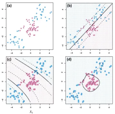
Figure 2.12 Example case of kernel functions application on non-linear data (a) data points with two categories, (b) SVM with linear kernel, (c) SVM with polynomial kernel, (d) SVM with radial kernel ... 19
Figure 2.13 Process of capturing the microseismic events (Quirein et al., 2006) ... 22
Figure 2.14 Process of the conventional microseismic data analysis ... 23
Figure 2.15 Correlation between SRV and 6-month cumulative gas production (Mayerhofer et al., 2006) ... 24
x
Figure 3.2 Workflow of the ANV calculation process ... 34
Figure 3.3 Example of the FRD calculation process ... 36
Figure 3.4 Workflow of the FRD calculation process ... 36
Figure 3.5 Schematic of well performance prediction model generation ... 37
Figure 3.6 Combinations of ERV tested during application process ... 38
Figure 4.1 Wells permitted or completed in the Eagle Ford Shale play ... 41
Figure 4.2 Geological location and distribution of the wells for Middle McCowen ... 42
Figure 4.3 Graphical representation of monitor well and geophones for well 9 and 12... 43
Figure 4.4 Daily oil production trend graph from the day started production for four wells ... 45
Figure 4.5 Distributed microseismic events for well 9 and 12 ... 46
Figure 4.6 Well-based separated shapes with input variables of magnitude, moment, and P to shear energy ratio, and event location coordinates ... 47
Figure 4.7 TDA shapes built based on correlation metric ... 49
Figure 4.8 TDA shapes built based on Euclidean distance metric ... 49
Figure 4.9 TDA model selected for the calculation of ANV ... 50
Figure 4.10 Graph showing a positive relationship of magnitude and moment ... 51
Figure 4.11 General process of cross validation using training and test dataset ... 55
Figure 4.12 Graphical representation of Leave-One-Out cross validation method ... 56
Figure 4.13 Schematic representation of the process in building a well performance predictive model ... 57
xi
Figure 4.15 Graphical representation of experiment 1 result ... 59
Figure 4.16 Graphical representation of experiment 2 result ... 60
Figure 4.17 Graphical representation of experiment 3 result ... 61
xii
Table 3.1 Attributes for the raw microseismic data ... 27
Table 3.2 Attributes for the processed microseismic data ... 28
Table 3.3 Attributes for the raw daily well production data ... 29
Table 3.4 Attributes for the processed well production data ... 30
Table 3.5 Attributes for the well trajectory data ... 30
Table 3.6 Attributes for the processed well trajectory data ... 31
Table 4.1 General treatment well data ... 43
Table 4.2 Calculated 18-month cumulative production ... 44
Table 4.3 Combinations of response variable and predictor variables used in the model generation ... 53
Table 4.4 Validation result of experiment 1 ... 58
Table 4.5 Validation result of experiment 2 ... 60
Table 4.6 Validation result of experiment 3 ... 61
Table 4.7 Validation result of experiment 4 ... 62
Table 4.8 Comparison chart of model accuracy through cross validation ... 63
1 CHAPTER I INTRODUCTION
1.1 Motivation
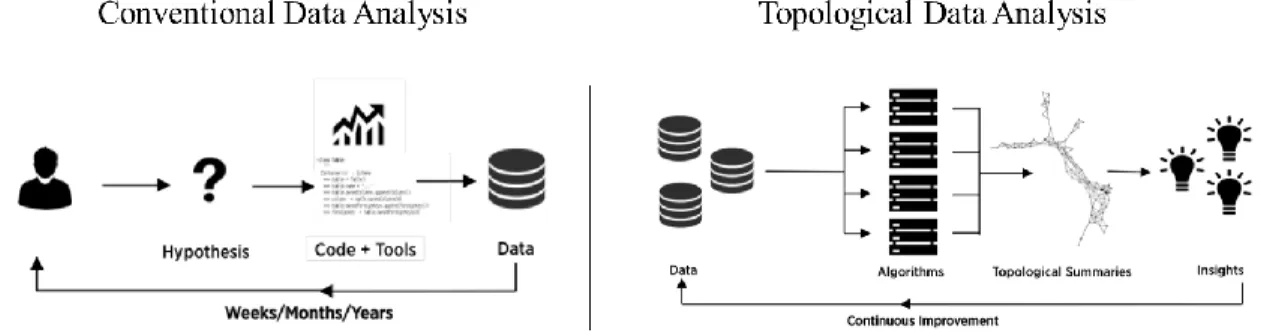
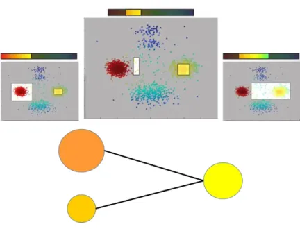
Recently, a huge amount of reservoir data has become available due to advances in data sensing and storage technologies. By analyzing reservoir data, we can gain a better understanding of reservoir description and ensure correctness of reservoir simulation. However, reservoir data is usually multi-dimensional and heterogeneous data, which requires labor intensive analyses, and sometimes the analysis results in an inaccurate performance. As shown in (Figure 1.1), while conventional data analysis approaches take a fair amount of time to appropriately analyze the data, the process including new data analytic methods can guide engineers to find insights from the data much faster and easier (Ayasdi, 2015).
Figure 1.1 Comparison between conventional data analysis and topological data analysis (TDA)
Nowadays, oil and gas industry is suffering from the prolonged low oil prices. Especially, development of shale reservoir was hit hard because of its high capital costs
2
that might exceed current oil price. Thus, maximizing profits through controlled the oil and gas production on occasion demands for shale reservoir have become more critical. Precise estimation in performance of a well is essential as it provides a guideline for decision making in production. To fulfill these needs, a new approach is presented to build an event-based well performance predictive model by analyzing the microseismic data.
For the microseismic data, there are around 3,000 microseismic events captured per well during hydraulic fracturing, but only one gas/oil production data is available. Thus, previously there was only a simple linear correlation model between Stimulated Reservoir Volume (SRV) and the cumulative gas/oil production from the well. This creates a different set of problems including low accuracy, especially when the sample size is small. Inspired from the fact that SRV is calculated based on the consideration of each microseismic event as shown in (Figure 1.2) (Microseismic Inc., 2015), this research explores a new technique of building a regression model based on each microseismic event for the well performance prediction. To increase the accuracy of the well performance predictive modeling, Topological Data Analysis (TDA) has been utilized for feature extraction of microseismic data to create a better representation value of each microseismic event and Support Vector Machine (SVM) has been utilized in building an actual predictive model and for the validation process.
3
Figure 1.2 Illustration of Stimulated Reservoir Volume (SRV) calculation based on microseismic events (Microseismic Inc., 2015)
1.2 Research Objectives and Thesis Outline
The objectives of the research include (a) to introduce two new attributes, Average Node Value (ANV) and Fracture Distance (FRD), from microseismic data that can give an ability to consider each microseismic event’s effect on the cumulative production of the well, (b) to build a prediction model that can estimate ultimate shale gas / tight oil production from a well utilizing these new attributes, and (c) to validate accurateness and robustness of the model through cross validation and find a future work that can be done for better performance. Now, we will outline the specific procedure of this thesis in Chapters II-V.
4
This research consists of three main parts. First, in Chapter II, we presented a background with literature review of data mining, machine learning, TDA, SVM, and microseismic analysis that are used for this study. Secondly, in Chapter III, we introduce two attributes along with data processing and methodology of obtaining and utilizing these attributes for event-based well performance model generation. Then, in Chapter IV, we implement this methodology to actual dataset from Middle McCowen, Eagle Ford, Texas and build a model based on the raw and generated dataset. Through leave-one-out cross validation method, four cases of the field case study have been validated through rank-order prediction results of the model. In Chapter V, the research is concluded with a summary of the key findings. Recommendations and proposals for further research are also presented.
5
CHAPTER II
BACKGROUND AND LITERATURE REVIEW
2.1 Introduction
In this chapter, background about concepts of machine learning and data mining is provided. In addition, a review of two data analysis techniques, Topological Data Analysis (TDA) and Support Vector Machine (SVM), which were utilized during model generation is presented, as well as a review of the how microseismic data has been previously analyzed as microseismic data has been used to the performance predictive model generation.
2.2 Data Mining and Machine Learning
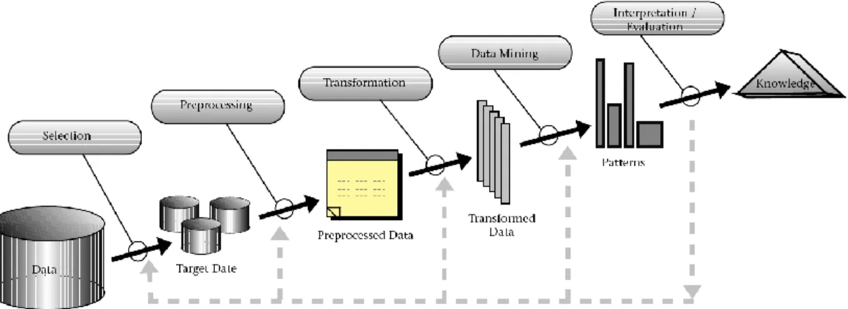
Data mining is about automating the process of searching for patterns in the data including association, sequence or path analysis, clustering, classification, regression, and visualization (Fayyad et al., 1996). Data mining is a crucial task within knowledge discovery in database (KDD), which is defined as the non-trivial process of identifying valid, novel, potentially useful, and ultimately understandable patterns in data as shown in (Figure 2.1). It improves the value of the complex data to assist the engineers in decision-making. In petroleum engineering, Data mining has been used in many areas including seismic data analysis, reservoir surveillance, and prediction (Bailey et al., 2013; De Jonge et al., 2002; Marroquin et al., 2009).
6
Figure 2.1 Process of knowledge discovery in database (KDD) (Fayyad et al., 1996)
On the other hand, machine learning is a method of data analysis that automates analytical model building (Tailor, 2015). It was born from pattern recognition and the theory that computers can learn without being programmed to perform specific tasks. As shown in (Figure 2.2), machine learning algorithms mostly falls into supervised learning method and unsupervised learning method. Unsupervised learning is used when the model is not provided with the correct results during the training. The main goal of unsupervised learning methods is to discover interesting facts about the measurements, such as if there is an informative way to visualize the data or subgroups among the variables or among observations can be discovered. Principal Component Analysis (PCA) is the most widely used unsupervised learning method, PCA is used for data visualization or data pre-processing before supervised methods are applied and clustering is used for discovering unknown subgroups in data. Supervised learning is used when training data includes both the input and the desired results. The main goal of supervised learning methods is to understand relationship between the input and the results and build a model based on it, it
7
would enable to predict the response when there is an additional input. Supervised learning problems can be further divided into regression and classification problems. Regression covers situations where response is continuous/numerical and classification covers situations where response variable is categorical. Linear regression is the most widely used supervised learning method as it is simple and easy to interpret.
Figure 2.2 Subgroups for machine learning algorithms
To understand how machine learning has been applied, a couple papers have been reviewed. In the paper written by Rosten et al (2010), authors tried to improve an existing corner detection tool, FAST, by implementing machine learning algorithms. They imposed each relative position of pixels (S_(p→x)) to three states, darker, similar, and brighter. Then a decision tree was created to choose which set of pixels would go into FAST tool for the corner detection. They tested the improved tool, FAST-9, to compare repeatability and speed from previous detector and conclude that implementing machine
8
learning algorithms produced significant improvements in repeatability and yielding a detector that is both very fast and high quality.
On the other hand, Pang and Lee (2002) tried to implement machine learning techniques (Naïve Bayes, maximum entropy classification, and SVM) to sentiment classification of movie reviews to see whether each review is positive or negative. But, for this case, machine learning technique couldn’t reach better result from traditional-topic-based-categorization technique due to the thwarted expectations (e.g., “a good actor trapped in a bad movie”). They concluded that building an ability to catch on-topic sentence in overall opinions would be future work to address the problem.
Among several trending machine learning algorithms, TDA and SVM have been chosen for this research. In the beginning, TDA has been considered because it already had a couple successful applications in petroleum engineering field. Thus, TDA’s ability of dimension reduction which is enabled by node/edge system generated by lens function made it more attractive. SVM is also included because while most of machine learning algorithms tend to necessitate big and complex data to guarantee the accuracy of model, SVM has relatively low threshold for size of data to obtain a model with accuracy (Chi, 2008). This characteristic of SVM expands possible usage of machine learning algorithms in more circumstances. Now, let’s look into the details of the papers that have applied TDA or SVM on petroleum engineering.
9 2.3 Topological Data Analysis
TDA provides a general framework for analyzing complex data. It draws on the concept that every data has shapes and the shapes have meanings, which can be driven to value. TDA creates a simple 2D or 3D graphical representation of complex multi-dimensional data with minimum data loss and robust to data noise. Graphical representation is based on topological network which is composed of nodes and edges, where a node is a group of similar data points and an edge is connection between nodes having a data point in common.
Topology was first introduced by the Swiss mathematician Leonhard Euler in the 18th century (Euler, 1741) and main goal of its initial applications was creating a simple representation to help solving a problem (Figure 2.3). Then, topology has been developed as an analysis method by Carlsson for the data analysis of complex multi-dimensional data (Carlsson, 2009).
Figure 2.3 Simple example of topology (Simanaitis, 2014)
There are three main characteristics of topology that made TDA feasible: coordinate-free representation, deformation invariance, and compressed representation.
10
Along with these characteristics, the fact that the shape of TDA is generated based on similar attributes in an overlapping fashion was critical for the study. To build an event-based well performance model, it is necessary for each events to have their own value of indicator. Thanks to TDA, we could obtain each event’s indicating value of the production. The detailed process of creating TDA shape is as follows.
In the generation of TDA shape, two important parameters, a metric and a lens, have to be selected. A metric is a measure of similarity (or distance) between data points and it is also called as distance function. Through metric selection, it can be decided that whether absolute value of the data points or rather some correlation or angle (in high dimensions) between the vectors representing the data points would be considered in positioning.
A lens is a filter that converts the dataset into a vector and determines how the dataset is partitioned for clustering and which aspect of the dataset should be emphasized. Each data point in the original dataset becomes a scalar element in the vector representing the dataset after performing a lens operation. A lens can be defined by selecting a column in a dataset or a function that can come from geometry or statistics, such as topological neighborhood and PCA. One or more lenses can be used simultaneously for the analysis of a dataset.
Additionally, there are two parameters of a lens to be determined, resolution and gain. Resolution controls the number of nodes that will be created by the lens operation; clustering than takes place within these nodes. By increasing resolution, the scope of each individual node is decreased. Gain is the extent to which the data will be oversampled.
11
This is the amount that each node will overlap with the adjacent nodes. A data point appears in the number of nodes, to which the gain is set. Reducing the value of gain will result in smaller groups of nodes and more singletons, unconnected nodes, while higher gain settings will show larger shapes with many connections between nodes.
Figure 2.4 Example case shown in 2D graph
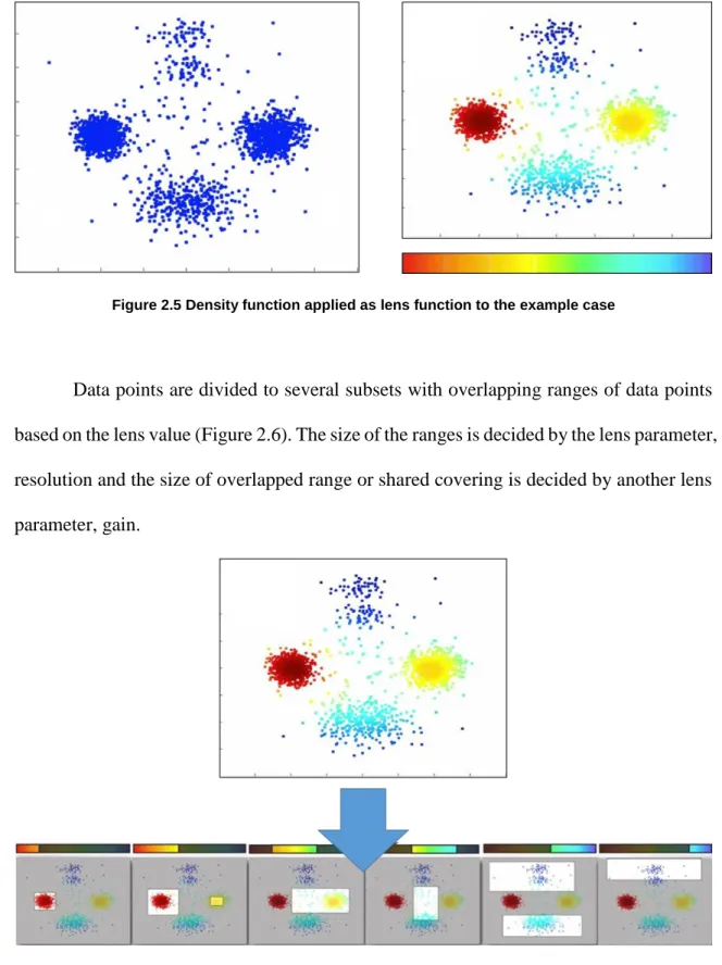
For better understanding of TDA process, simple example case of 2200 data points with 2 columns is provided below (Ayasdi, 2015). Euclidean distance has been selected for the distance function and Density function has been selected for the lens in this process. First, (Figure 2.4) shows the two dimensional graph where each data points are displayed using a distance function. Then, lens has been applied to each data point and it has been colored based on the value after applying lens function (Figure 2.5), which is magnitude of density in this case. Red color indicates high density and blue color indicates low density of data points nearby.
12
Figure 2.5 Density function applied as lens function to the example case
Data points are divided to several subsets with overlapping ranges of data points based on the lens value (Figure 2.6). The size of the ranges is decided by the lens parameter, resolution and the size of overlapped range or shared covering is decided by another lens parameter, gain.
13
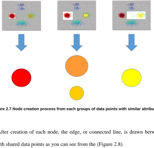
Each group of data points with similar lens value and similar position from distance function becomes one node as shown in (Figure 2.7). In this case, representing lens value has been used for the node’s coloring and the size of data points included in each node decided the node’s size.
Figure 2.7 Node creation process from each groups of data points with similar attributes
After creation of each node, the edge, or connected line, is drawn between the nodes with shared data points as you can see from the (Figure 2.8).
14
Figure 2.8 Edge connection between nodes with overlapping data points
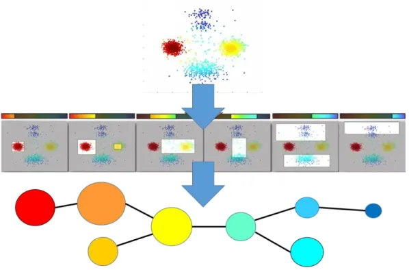
To sum up, the final representation of 2,200 data points that is generated from the process of TDA with density lens and Euclidean metric is provided below in (Figure 2.9).
15
Figure 2.9 Whole process of TDA applied on example case
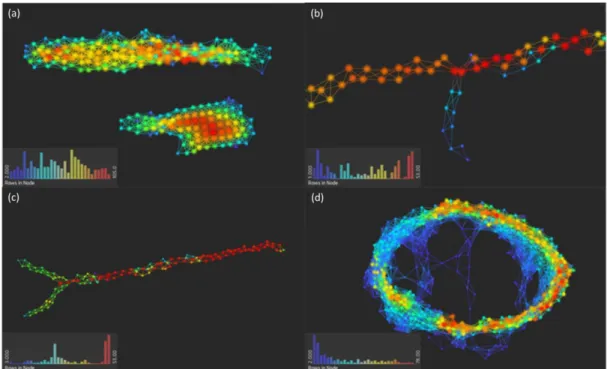
From the output of the TDA, there are some characteristic shapes such as clustered compartmentalization, flare, which indicates anomaly from the center, Y-junction, and loop that are easy to understand. Actual example of output images are on (Figure 2.10). As mentioned above, reduced dimensional visualization helps engineers to view and understand the data by shape itself with ease.
16
Figure 2.10 Examples of TDA output (a) Clustered (b) Flare (c) Y-junction (d) Loop
A growing number of large companies and institutional organizations have successfully adopted the TDA for addressing a wide variety of data-driven problems. Main research fields, to which TDA has been applied, include genetics, pharmaceutics, healthcare, finance, energy, security, and defense (Cortis, 2015).
There are a limited number of studies conducted on petroleum engineering area using TDA. Alfaleh (2015) conducted a study on the reservoir connectivity and compartmentalization by analyzing an inverted 4D time-lapse seismic datasets on Brillig and Norne fields using the TDA. This compartmentalization was tested because accurate compartmentalization ensures the precision of forecasts and development plans, the correctness of reservoir simulation. TDA was able to compartmentalize the reservoir models with various process configurations.
17
Also, Cortis (2015) studied lithofacies characterization of the Marcellus shale gas formation using data set of petrophysical logs of composition (quartz, calcite, clay, and total organic carbon) and elastic parameters (density, and compressional and shear velocity) on four geological sections. This study was initiated because there was a part that lies on the boundary of conventional separation methods (using the AI-PR plane or using dendrogram representation of the data) and these couldn’t be separated without a specified priori which is instable. The application of TDA to well logs in the Marcellus Formation successfully provided clear identification of four geologic layers of focus.
Unlike the previous studies on the application of TDA to petroleum engineering, which were focused on the classification or clustering the data, the objective of this research through TDA is to discover the hidden information by utilizing quantitative value of each node, such as representative node value of 18-month cumulative tight oil production data with the given datasets.
2.4 Support Vector Machine
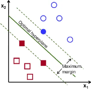
SVM is one of the supervised learning method in machine learning that tries to find an optimal separating hyperplane from training dataset. The operation of the SVM algorithm is based on finding the hyperplane that gives the largest minimum distance to the training examples, so the optimal separating hyperplane maximizes the margin of the training data (Figure 2.11) (OpenCV, 2016). SVM is based on the statistical theory of VC dimension (Vapnik-Chernovenks Dimension) and the theory of structural risk minimization. SVM has strict theoretical basis, and can better solve the small sample,
18
nonlinear and high dimension and local minimum point and other practical problems (Aibing et al., 2012). The decision function is fully specified by a subset of training dataset, the support vectors (Deng et al., 2012). As SVM has been developed, it has ability to separate the patterns that are not linearly separable by transformation of original data by mapping into new space using kernel function.
Figure 2.11 Illustration of finding the optimal hyperplane (OpenCV, 2016)
The original SVM algorithm was initially introduced in Russia in the early 1960s (Vapnik and Lerner, 1963; Vapnik and Chervonenkis, 1964). The SVM algorithm has been further developed at AT&T Bell Laboratories by Vapnik and coworkers in mainly two perspectives; (i) a way of creating nonlinear classifiers by applying kernel function in 1992, and (ii) utilization of soft margin in 1993 (Boser et al., 1992; Guyon et al., 1993). It have gained its fame in early 2000s with excellence in performance of pattern recognition.
19
While maximum margin classifier is used when classes were separable by a linear boundary that was not the case for most of real-world situations. Thus, support vector classifier with soft margin has been introduced for the situation that there is no solution as the observation classes are mixed. Soft margin allows some violation of margin and the budget of allowed margin violation is decided by tuning parameter, cost (C). The optimal hyperplane is determined only by the support vectors, which are group of points that lie on the margin or on the wrong side of the margin. Furthermore, kernel function has been introduced to extend to non-linear class boundaries. As it is depicted in (Figure 2.12), using polynomial kernel or radial kernel, SVM gained ability to separate non-linear decision boundary cases (James et al., 2013).
Figure 2.12 Example case of kernel functions application on non-linear data (a) data points with two categories, (b) SVM with linear kernel, (c) SVM with polynomial kernel, (d) SVM with radial kernel
20
There were no specific literatures that have performed SVM/SVR on microseismic data but if we look on whole petroleum engineering, several studies have been performed. Al-Baiyat and Heinze (2012) conducted a study on the prediction of stuck pipe occurrence by analyzing a database that includes mud properties, directional characteristics, and drilling parameters using the Artificial Neural Networks (ANN) and SVM. This study involved classifying stuck pipe incidents into two groups – stuck and non-stuck – and also into three subgroups: differentially stuck, mechanically stuck, and non-stuck. This study demonstrated that both ANNs and SVMs are able to predict stuck pipe occurrences with reasonable accuracy, over 85%.
Al-Anazi and Gates (2010) studied feasibility of SVR method in permeability prediction for a heterogeneous reservoir with log data, which includes gamma ray, neutron porosity, sonic porosity (DT), bulk density, and formation resistivity. This study was initiated because even there were some applications of neural-network-based methods for permeability correlation, these methods have limited generalizability and that usually led the global correlations to be less accurate compared to local correlation. By comparing results of predicted permeability from various machine learning algorithms (SVR, multilayer perception (MLP), generalized neural network (GRNN), and radial-basis-function neural network (RBFNN)) with several accuracy measures (Correlation coefficient, root-mean-square error (RMSE), absolute-average error (AAE), and maximum absolute error (MAE)), accurateness and robustness of SVR method were revealed.
21 2.5 Microseismic Data Analytics
There were several factors that led to shale gas boom in the past decade of 2000s which enabled firms to produce shale gas profitably, including technology innovation, government policy, market structure, favorable geology, and natural gas pipeline infrastructure. Among these factors, the main driver was definitely technology advancement that were developed from government research and development programs and the oil industry for use in oil exploration and production (Wang and Krupnick, 2013). The key technologies were horizontal drilling that enabled well to stay in the pay zone of reservoir for longer distance and hydraulic fracturing that enabled increase production zone by generating fracture in the closed tight reservoir.
Microseismic data of hydraulic fracturing is captured from microearthquakes or acoustic emissions associated with either fracture creation or induced movement of pre-existing fractures (Urbancic et al., 1999). Typically, the detection uses geophones in a well temporarily used as an observation well as depicted in the (Figure 2.13). Which means microseismic events captured indicates the fracture to the near-wellbore zone with stimulation of productivity by releasing trapped oil/gas.
22
Figure 2.13 Process of capturing the microseismic events (Quirein et al., 2006)
Thus, microseismic monitoring is technology that can be used for characterizing fracture network created from fluid injection and hydraulic fracturing (Tafti and Aminzadeh, 2012). Several authors (Fisher et al., 2004; Downie et al., 2009; Barree et al., 2002; Warpinski et al., 2005; Tezuka et al., 2008) have studied about microseismic methods in fracture detection. These authors have also tried to correlate production data with the dimensions of the microseismic clouds and volume estimates based on the density of microseismic events (Tafti and Aminzadeh, 2012). Analysis of microseismic data helps in better understanding of completions design, and parameters, and in recent years, examples of such applications are abundant (e.g., Duncan and Williams-Stroud, 2009; Eisner et al., 2010; Lakings et al., 2006; Vermylen and Zoback, 2011) (Gangopadhyay et al., 2013).
23
In conventional reservoirs and tight gas sands, single-plane-fracture half-length and conductivity are the key drivers for stimulation performance. In shale reservoirs, where complex network structures in multiple planes are created, the concepts of single-plane-fracture half-length and conductivity are insufficient to describe stimulation performance. So, SRV is used as a correlation parameter for well performance. (Figure 2.14) shows general workflow of analyzing microseismic data using SRV.
Figure 2.14 Process of the conventional microseismic data analysis
While the effectively producing network could be smaller by some proportion, it is assumed that the created and the effective network are directly related. However, SRV is not the only driver of well performance (Mayerhofer, 2010). Fracture spacing and conductivity within a given SRV are just as important (Cipolla and Wallace, 2014). Thus for this research, rather than expanding the parameters of fracture spacing and conductivity in addition to microseismic data, model was generated for near-by wells in same region with the assumption that their characteristic in fracture spacing and conductivity would be the roughly same. Graph provided below (Figure 2.15), shows the case where SRV has been successfully correlated with cumulative gas production data
24
from shale gas reservoir in Barnett Shale (Mayerhofer et al., 2006). Fisher et al. (2004) also detailed microseismic-fracture-mapping results for horizontal wells in the Barnett shale. This work illustrated that production is related directly to the reservoir volume stimulated during the fracture treatment.
Figure 2.15 Correlation between SRV and 6-month cumulative gas production (Mayerhofer et al., 2006)
Mayerhofer et al. (2006) also performed numerical reservoir simulations to understand the impact of fracture-network properties such as SRV on well performances (Figure 2.16). This paper showed that well performance can be related to very long effective fractures, forming a network inside a very tight shale matrix of 100 nanodarcies or less.
25
Figure 2.16 Numerical simulation result testing the effect of stimulation on well performance (Mayerhofer et al., 2006)
26
CHAPTER III METHODOLOGY
3.1 Overview
This chapter describes the methodology we used in this study to build the event-based well performance predictive model using microseismic data in shale reservoir. In order to achieve this goal, two new attributes were calculated from the raw dataset of microseismic data, daily well production data, and well trajectory data. In the meantime, we tried to obtain ideas from existing data analytics methods while developing the methodology. In section 3.2, how raw dataset have been pre-processed before actual generation of the new attributes is given. Then the process of generating two new attributes, Average Node Value (ANV) and Fracture distance (FRD), using pre-processed dataset has been introduced in section 3.3. Finally in section 2.4, new concepts of Event Representation Value (ERV) and Well Representation Number (WRN) is provided and how these have been included in well performance model generation through SVM and how results of the model have been compared has been presented.
3.2 Data Generation and Data Preprocessing
This section details the preparation of the raw dataset, which includes microseismic data, daily well production rate data, and well trajectory coordinates data, before these data have been used for the new attributes generation. Along with the preparation for the actual new attributes generation, input properties from each dataset has
27
From microseismic data, there are following attributes as shown in (Table 3.1). Depending on the time frame when the microseismic data have been captured, there were some attributes that are not consistently provided in the raw dataset of each well. So these variables have been excluded through pre-processing from this study to maintain its universality for future applications.
Table 3.1 Attributes for the raw microseismic data
Attribute Name Description
JobTime Time format: DD:MM:YY:HH:MM:SS
MS_EVENT_ID Sequential unique number identifying individual events MS_EVENT_TYPE Processing identifier used to flag visualization software: 0 is
normal event; 2 is bad event; 3 is recomputed event MS_LOC_SNR Signal to noise ratio after orientation of P&S to computed
location- higher is better quality data
MS_DET_SNR Signal to noise ratio after orientation of P&S to target location- higher is better quality data
QC_LOC_X X location relative to reference - treatment well surface location
QC_LOC_Y Y location relative to reference - treatment well surface location
QC_LOC_Z Z location relative to reference - mean sea level
QC_DISTANCE Distance from event to middle of receiver array
PSH_AMPL_RATIO Average ratio of P amplitude/Shear Amplitude around 1st breaks of each shuttle by event
NOISE_LEVEL Computation of average RMS to give indication of
28
SP_RADIUS Source parameter - computed radius of source
SP_MOMENT Source parameter - computed moment of source
SP_STRESS_DROP Source parameter - computed stress drop of source; change in stress state, generally largest at bed boundaries
SP_MAGNITUDE Source parameter - computed magnitude of source
SP_ENERGY Source parameter - computed energy of source
Raw microseismic data was initially separated in each stages as a spreadsheet, so it was combined together as a whole well’s microseismic data, and then it was again combined as a whole case for the targeted wells. After the data from all wells were embed, some properties have been normalized of the columns for the improvement in analysis by reducing overemphasizing of an attribute. Also, some apparent attributes that weren’t going to be used for our study, such as event id and job time, was removed during processing job. After preprocessing of microseismic dataset, the following columns provided in (Table 3.2) has been organized for the next step.
Table 3.2 Attributes for the processed microseismic data
Attribute Name Description
QC_LOC_X X location relative to reference - treatment well surface
location
QC_LOC_Y Y location relative to reference - treatment well surface
location
29
PSH_NORM Normalized value of PSH_AMPL_RATIO
MOMENT_NORM Normalized value of SP_MOMENT
MAGNITUDE_NORM Normalized value of SP_MAGNITUDE
From the daily well production rate data of each well, following attributes shown in (Table 3.3) were available from the spreadsheet.
Table 3.3 Attributes for the raw daily well production data
Attribute Name Description
PROD_DT Date of production
OIL_PROD Daily production rate for the oil
GAS_PROD Daily production rate for the gas
WAT_PROD Daily production rate for the water
TUBING_PRESS Pressure of tubing
CASING_PRESS Pressure of casing
Depending on well’s major type of production, either oil or gas production could be applied for the model generation. As we have covered in chapter I, our goal was to estimate the ultimate well performance from the microseismic data. However, 18-month was the longest time frame that covered duration of provided production data from all
30
wells that were considered for this study. Thus, we’ve calculated 18-month cumulative production value for both oil and gas and set it as new columns for each well (Table 3.4).
Table 3.4 Attributes for the processed well production data
Attribute Name Description
CUM_OIL_PROD 18-month cumulative production for the oil
CUM_GAS_PROD 18-month cumulative production for the gas
Finally, from the well trajectory data for each well, following columns shown in (Table 3.5) were available.
Table 3.5 Attributes for the well trajectory data
Attribute
Name Description
X X location relative to reference - treatment well surface location Y Y location relative to reference - treatment well surface location
Z Z location relative to reference - mean sea level
MD the measured depth along the planned well path
INCL well bore inclination at MD
AZIM angle of the well bore direction as projected to a horizontal plane and relative to due north.
DX Difference between current X and previous X
DY Difference between current Y and previous Y
31
As our goal for this study was to consider an effect of hydraulic fracturing through the microseismic data, only well trajectory’s horizontal part should’ve been considered for the calculation. Thus, the well trajectory has been filtered to coordinates with inclination of over 80 degrees to ensure the only horizontal part of the well is used for the future calculation. After filtration of each well, x, y, and z coordinates values of each well have been taken from the data for the future calculation in the new attribute generation (Table 3.6).
Table 3.6 Attributes for the processed well trajectory data
Attribute
Name Description
X X location relative to reference - treatment well surface location Y Y location relative to reference - treatment well surface location
Z Z location relative to reference - mean sea level
These pre-processed variables shown in Table 3.2, 3.4, and 3.6 have been separated into two situations (section 3.3.1 and 3.3.2) for the calculation of each new attributes.
32 3.3 Feature Extraction
3.3.1 Average Node Value
The objective of this section is to give an overview on the process of obtaining the Average Node Value (ANV) with utilization of TDA. The definition and physical meaning of ANV is introduced in section 3.3.1.1 Then, the steps of obtaining ANV through actual TDA process is summarized.
3.3.1.1 Definition of Average Node Value
As it has been mentioned in previous sections, one well only has a single production value even there are around three thousands of microseismic events available. Consideration for event-based effect on well performance would be a meaningful approach to improve the accuracy of model generation. As it was shown during background study of TDA, TDA has a characteristic of grouping events with similar attributes that shows similar lens values and put them in a node. Furthermore, due to the overlapping nature of TDA for the connection between nodes, one event will fall into several nodes with different combinations of events that have similar characteristics. Which means, if we utilize TDA accordingly, we would be able to create a new term called ANV that has physical meaning of average oil production from combinations of microseismic events with similar attributes that can represent effect of the microseismic event for the production.
33 3.3.1.2 Process of TDA for Average Node Value
As the main goal of TDA is extracting meaningful information from the shape of the data, the process of building shape graphs and how ANV is calculated from the shape is introduced. First step was to evaluate different metrics and lenses performance to find a combination of metrics, lenses, and input variables that led to separate the trends of high production nodes from the trends of low production nodes.
Even one simple modification from a combination of metrics, lenses, and input variables led to a dramatic change in a shape of TDA. Thus, we decided to test the results by changing the combinations in the order of input variables, distance metrics, and a function of lens. The targeted shape was the shape that showed specific shapes introduced in (Figure 2.10) that has characteristic meanings in background study of TDA, such as flairs, cycles, or clusters along with the ability to separate the production trends. Details of finding the appropriate combination is provided in application section 4.2. After each combinations of metrics, lenses, and input variables have been investigated, the TDA shape that shows an ability to separate microseismic events based on production with stability has been selected.
34
Figure 3.1 Example of the ANV calculation process
As it can be seen from (Figure 3.1), where simple example of obtaining ANV value through TDA is depicted, ANV will be calculated by (1) tracking down which nodes each event has fell into, then (2) organizing the cumulative production value of each nodes, and lastly (3) calculating an average value between these cumulative production value of nodes that each event has fell into. Workflow is also provided in (Figure 3.2).
35 3.3.2 Fracture Distance
The objective of this section is to give an overview on the process of obtaining the Fracture Distance (FRD) with simple calculation of distance. The definition and physical meaning of FRD is introduced in 3.3.2.1. Then, the steps of obtaining FRD through actual distance calculation process is summarized.
3.3.2.1 Definition of Fracture Distance
Fracture Distance (FRD) is the distance from the well trajectory to microseismic event, which can be used to estimate how far hydraulic fracturing had effected in the formation. As far as microseismic event stays in the “pay zone” part of the reservoir, the farther distance from the horizontal part of the well indicates the better hydraulic fracturing stimulation on that region of the reservoir.
3.3.2.2 Process of Calculation for Fracture Distance
As FRD is just a simple indication of distance from the well to microseismic event, its calculation is also a simple process. However, as real field’s well trajectory is not a perfect line or a given equation, each points of horizontal part should be considered for the calculation. To keep our process data-driven, distance between each microseismic events and horizontal trajectory points of its well are calculated and the minimum value has been set as FRD value of the microseismic event. There are about 70 horizontal trajectory points that are given as a raw data for each well, but accuracy could be improved if we generate additional in-between points with given trajectory points if necessary. Same
36
as ANV, along with the figure representation of simple case in (Figure 3.3), workflow is also provided in (Figure 3.4).
Figure 3.3 Example of the FRD calculation process
Figure 3.4 Workflow of the FRD calculation process
3.4 Model Generation
As it has been mentioned in previous chapter, goal of this research is to generate a well performance predictive model with high accuracy by understanding each microseismic events effect on production. Thus, the value that represents indicator for effects on well performance is defined as Event Representation Value (ERV) and
Well-37
scale indicator that combined ERV has been defined as Well Representation Number (WRN) (Figure 3.5).
Figure 3.5 Schematic of well performance prediction model generation
3.4.1 Event Representation Value
Event Representation Value (ERV) is defined as a value that can depict the effect of a single microseismic event on the ultimate production of the well. In this study, while ANV, new attribute obtained through TDA process, has been fixed as a part of ERV, several combinations and normalization methods have been tested to obtain the combination that leads to the most accurate well performance modeling. As shown in (Figure 3.6), three specific combinations have been tested for the study, (i) 0-1 normalized ANV, (ii) 0-1 normalized ANV multiplied with 0-1 normalized FRD, and (iii) normalized ANV multiplied with 0-1 normalized FRD. ERV will be used as response variable in the modeling. Thus, the accuracy between combinations will be compared during validation process of the application.
38
Figure 3.6 Combinations of ERV tested during application process
3.4.2 Well Representation Number
Each well has thousands of microseismic events that are captured during hydraulic fracturing, which means there are also thousands of ERVs for a well. Thus, we needed to select a single number that can represent thousands of numbers properly. We defined this number as Well Representation Number (WRN). After considering several representation values, such as median, mean, mode, and standard deviation, average value of the ERVs has been considered as WRN in this research. The fact that other machine learning algorithm of decision tree uses mean value as a represent value for the subset also affected in using mean value for WRN.
3.4.3 Process of Well Performance Prediction Model Generation
After the calculation of ERVs from the training dataset, SVM (SVR) method was utilized in building the well performance predictive model. For each of the microseismic events, combinations between Magnitude, Moment, P to Shear Energy Ratio, FRD was selected as the predictor variable and ERV as the response variable. Actual combinations that were used for building a model are provided in application section 4.3. SVM (SVR)
39
method has been selected as a model generation algorithm because (1) it is most commonly used machine learning algorithm for classification since its introduction in 2000s and (2) it has relatively small threshold of data size for model accuracy compared with other machine learning algorithms (Chi, 2008). It could be tested with other machine learning methods such as random forest or neural network to improve the accuracy of the model. Application of SVR was performed on R with e1071 package.
In the next chapter, we will actually apply this methodology of building well performance predictive model on the field case of Middle McCowen, Eagle Ford, Texas. Then, it would be validated through the cross-validation of leave-one-out method to ensure its improvement in accuracy.
40
CHAPTER IV
APPLICATION TO MIDDLE MCCOWEN WELL
4.1 Introduction and Site Description
The objective of this chapter is to present the application of the methodology on the selected dataset. Actual field data from Middle McCowen well was used for the model generation and the validation in this study. Overview of the Eagle Ford region and Middle McCowen well is provided in this section. Then, the process of creating a shape through TDA and ANV calculation is provided. Actual model generation using SVM is given in section 4.3 and the cross-validation method that was applied for the validation of the methodology is provided. Finally, results and discussion from prediction performance evaluation is presented in section 4.5.
4.1.1 Model Description
Eagle Ford Region refers to the South Texas region where Eagle Ford Shale underlies its ground. Eagle Ford’s first producing well was developed by Petrohawk Corporation in 2008. Since then, thousands of wells have been drilled and the Eagle Ford Shale play have stretched to roughly 50 miles wide and 400 miles long. Eagle Ford Shale became one of the most actively drilled targets for oil and gas in the United States in 2010. These days, the Eagle Ford Shale contains 22 active fields across the play and average daily production of oil is 1,200 thousand barrels per day and average daily production of gas is 6,000 million cubic feet per day in 2016 according to U.S. Energy Information
41
Administration’s Eagle Ford Region Drilling Productivity Report. Wells permitted or completed in the Eagle Ford Shale play on May, 2016 is shown (Figure 4.1).
Figure 4.1 Wells permitted or completed in the Eagle Ford Shale play
Middle McCowen wells are located in Atascosa County of the Eagle Ford Region, Texas. First active production in Middle McCowen was started in 2011 and there are currently 74 wells (Figure 4.2). While Eagle Ford is mainly famous for shale gas production, Middle McCowen field’s main type of production is tight oil. Thus, tight oil instead of shale gas was considered for the well performance model generation.
42
Figure 4.2 Geological location and distribution of the wells for Middle McCowen
4.1.2 Data Description
In this study, three types of data from Middle McCowen have been utilized; (i) microseismic data, (ii) well daily production data, and (iii) well trajectory data. While there were 74 wells in Middle McCowen field, only 8 well data has been provided by Marathon Oil. Among 8 wells, only 4 wells have been actually hydraulic fractured and microseismic data has been captured during hydraulic fracturing. So, this case study has application to the limited number of wells, well 1, 4, 9, and 12.
Microseismic data was collected during the stimulation treatment of a well using a monitor well (Middle McCowen 3H) monitoring method for well 1 and well 4. Microseismic data from well 9 and well 12 was monitored from the vertical portion of the Middle McCowen 11H. In both cases, an array of 12 VSI geophones, spaced 100 feet apart
43
in vertical orientation, was used in monitoring. Graphical representation of monitor well and geophones for well 9 and 12 is provided in (Figure 4.3). Also, the general treatment well data is shown in (Table 4.1).
Figure 4.3 Graphical representation of monitor well and geophones for well 9 and 12
Table 4.1 General treatment well data
1H 4H 9H 12H
Well Type Horizontal Horizontal Horizontal Horizontal
Completion Perf/Plug Perf/Plug Perf/Plug Perf/Plug
KB (ft) 300 311 311 311 Total Meseaured Depth (ft) 16802 16670 18076 18014 Maximum Vertical Depth (ft) 11113 11108 11059 11082 Casing Data 5-1/2" 20lb/ft 5-1/2" 20lb/ft 5-1/2" 20lb/ft 5-1/2" 20lb/ft
44
As a result, around 3,000 microseismic events per well (well 1: 3,634 events, well 4: 3,158 events, well 9: 828 events, and well 12: 2,266 events) were captured during hydraulic fracturing process. Details of attributes have been explained in the section 3.2 and some attributes were eliminated during pre-processing as some raw data didn’t contain them.
When we look at the raw daily production data, it was captured from 9/16/2011 to 4/23/2014. However, well 9 and 12 have started their production from 9/14/2012. We had to limit our cumulative production value to 18-month as it was the longest time-frame that covered all the wells. Thus, 18-month cumulative oil production value instead of ultimate production has been used for the model generation of well performance prediction. Daily tight oil production rate trend for all of four wells with x-axis as days from the production started is shown in (Figure 4.4). After calculation of 18-month cumulative production for each wells, the result came out as shown in (Table 4.2). Well 1 showed the highest tight oil production during the time frame among all and well 4, well 9, and well 12 followed in an order.
Table 4.2 Calculated 18-month cumulative production
18-month Cumulative Production
1H 4H 9H 12H
45
Figure 4.4 Daily oil production trend graph from the day started production for four wells
Finally, in the raw well trajectory data, there were 173 coordinate points for well 1, 200 points for well 4, 194 points for well 9, and 176 points for well 12. After the filtration for the points with inclination over 80 degrees to obtain the horizontal part of the well trajectory, well 1 had 66 points, well 4 had 66 points, well 9 had 83 points, and well 12 had 73 points. As mentioned previously, each points could be doubled by adding in-between points of the coordinates to increase the accuracy of the distance calculation. However, it has not been applied due to consideration of the increase in calculation cost. Actual positions of microseismic events along with the well trajectory for well 9 and well 12 is shown in (Figure 4.5).
46
Figure 4.5 Distributed microseismic events for well 9 and 12
4.2 TDA Graph Creation and Analysis
For the calculation of ANV, TDA shape graph should be created beforehand. Aforementioned in the methodology, we have to find a combination of input variables, metric, and lens that can separate the trend of cumulative production value with the stability. Thus, the steps taken to find a right combination and to create the shape from the data are explained. Then, actual ANV calculation process is presented. During this study, TDA figures have been generated using Ayasdi Python SDK version 4.3.1 (ayasdi.com) and Ayasdi Core software version 1.59.
We tried to find a combination by changing factors in order of input variables, metric, then lens. Choosing input variables is challenging, but critical process. We have tested two combinations of input variables: (i) magnitude, moment, and P to shear energy ratio and (ii) magnitude, moment, and P to shear energy ratio, and event location coordinates. Among two combinations, the first combination without event location coordinates generated the easier to interpret shapes while the second combination generated shapes that were too focused on coordinates itself even with various
47
combinations of lens and metric have been tested. These coordinate-focused characteristic led the shapes to be separated by the wells. Shapes for second case, input variables with magnitude, moment, and P to shear energy ratio, and event location coordinates, are shown in (Figure 4.6). First shape was created with the metric of correlation and neighborhood lenses as lens function and second shape was created with the metric of correlation and MDS coordinates as lens function.
Figure 4.6 Well-based separated shapes with input variables of magnitude, moment, and P to shear energy ratio, and event location coordinates
With magnitude, moment, and P to shear energy ratio as an input variable, various metrics and lenses have been tested. While a metric defines the distance between all the data points in our dataset, a lens decides which aspect would be focused from the multidimensional dataset. Thus, these selection is also critical part of feature selection.
48
Various metrics have been tested with the fixed input variables, such as, Euclidean distance, correlation, angle, and cosine. Building a shape with non-normalized attributes showed a failure of these metrics as there was scale difference between columns that led to biased result of distance calculation. However, as attributes in input variables have been normalized during data pre-processing, problem was already addressed.
Then, one or more lenses of statistical functions were applied to the dataset, in particular, k-nearest neighborhood, PCA, and Gaussian Density function. Also, these functions has been tested with different parameters of resolution and gain to see how well production trend has been separated. Successful lens created stable shapes that showed an ability to separate high production and low production.
Following (Figure 4.7 and Figure 4.8) show the TDA shapes that were generated during testing various lenses and metrics. Shape (1), (2), (3), (4) was built based on correlation metric and (5), (6), (7), (8) was built based on Euclidean metric. Shape (1) used MDS coordinates as lens function, shape (2) and (5) used L-infinity Centrality and Gaussian density function as lens function, shape (3) and (6) used L-infinity centrality as lens function, shape (4) and (8) used neighborhood lenses as lens function, and shape (5) used PCA coordinates as lens function. First four shapes were closer to our goal of finding a characteristic shapes, while later four showed rather big and broad shape. Thus, first four shapes were considered for the future investigation. Then, among four shapes, shape (4) showed the most clear and concise separation trend in showing colors of cumulative oil production value. Shape (4) has been chosen as our final TDA model in this study.
49
Figure 4.7 TDA shapes built based on correlation metric
50
After each combinations have been investigated, the cycle shape (Figure 4.9) generated from the input variables of Magnitude, Moment, and P to Shear Energy Ratio, in metric of Norm Correlation and a set of lens functions of nearest neighborhood 1 and nearest neighborhood 2 showed stable results from the datasets. It was confirmed quantitatively through running statistical comparisons between two nodes groups that represented high and low trend of productions, the properties that creating the shapes were identified. Kolmogorov Smirnov (KS test) and Student’s t-test has been used for this statistical comparison.
51
Also, the loop shape created through TDA usually means that there is a positive relationship between two attributes and this relationship have been emphasized through lens function. Thus, we wanted to understand which attributes have been emphasized and as it is shown in (Figure 4.10), the loop shape was created through this process as the relationship between magnitude and moment has been emphasized.
Figure 4.10 Graph showing a positive relationship of magnitude and moment
After generation of the TDA shape with input variables of Magnitude, Moment, and P to Shear Energy Ratio, in metric of Norm Correlation and a set of lens functions of nearest neighborhood 1 and nearest neighborhood 2 on Ayasdi python package, each node have been colored by the average 18-month cumulative oil production value from the events consisting each node. Then, each node’s representing node value has been
52
extracted. On the other hand, events contained in each node is also obtained. From the two tables of events and values related to each nodes, ANV could be easily calculated using simple matlab code.
4.3 SVM Model Generation and Parameter Selection
After obtaining ANV and FRD from the raw dataset, well performance predictive model for oil and gas could be created. Model generation has been performed using SVR method. SVR has been selected for the model generation as it has power to fit a data with small number of events well, while other machine learning algorithms require high thresholds regarding the size of data. SVR has been performed on R using package e1071. With the definition that ERV is a value that has an ability to represent the effect of each microseismic events on ultimate production of the well, ERV has been set as a response variable in the model generation. To obtain the most accurate model and ERV, several combinations and normalization methods have been tested. The detailed predictor and response variable tested is shown in (Table 4.3). All the variables have been normalized in zero mean one standard deviation manner except the terms that have 01 behind their name. These has been normalized in 0-1 manner to stay in positive values through multiplication. The predictive model for case 1 was built based on the raw data of cumulative oil production. It was specified for comparison with the proposed model.
53
Table 4.3 Combinations of response variable and predictor variables used in the model generation
No. Response Variable
(ERV) ~ Predictor Variable
1 Cumulative Oil
Production Moment Magnitude PSh_ratio FRD_01
2 ANV_01 * FRD_01 Moment Magnitude PSh_ratio FRD_01
3 ANV_01 Moment Magnitude PSh_ratio FRD_01
4 ANV_01 * FRD_01 Moment Magnitude PSh_ratio
5 ANV * FRD_01 Moment Magnitude PSh_ratio FRD_01
6 ANV * FRD_01 Moment Magnitude PSh_ratio
Training data spreadsheet has been generated with the columns of Cumulative Oil Production, normalized Moment, normalized Magnitude, normalized P to shear energy ratio, 0-1 normalized ANV, 0-1 normalized FRD, normalized ANV * 0-1 normalized FRD, 0-1 normalized ANV * 0-1 normalized FRD to cover every combinations. On the other hand, for future validation, test data spreadsheet should contain normalized Moment, normalized Magnitude, normalized P to shear energy ratio, and 0-1 normalized FRD.
For the actual model generation using SVM, kernel and cost value should be chosen beforehand. There were several options for kernels, such as linear, radial, or polynomial, and linear kernel was used for this model generation because of the fact that as we have seen on previous microseismic data analytics, SRV showed linear relationship between the cumulative production values. For the cost value, which decides how much
54
violations will be accepted during building a model, there is a function that finds the cost that leads to the model with the lowest error. However, through tests with variation of cost values from 0.01 to 100, the results changed less than 1%, so we decided to use a value of 1 as the cost of the model generation.
To sum up, we’ve built 6 cases of well performance predictive model with different response and predictor variable using SVR method with linear kernel function and the cost parameter as 1 from the training dataset.
4.4 Prediction Performance Evaluation
We have chosen to use the dataset from Eagle Ford Middle McCowen for this study. As there wasn’t any additional data from near-by wells available for us to validate this method, we chose to validate introduced methodology using the cross-validation method on the original data from 4 wells. The cross-validation method validates the methodology by separating a dataset into training and test dataset. The simple illustration of the cross-validation is shown (Figure 4.11).
55
Figure 4.11 General process of cross validation using training and test dataset
Model would be built based on the training dataset. Then, predictor variables of test dataset would be put into generated model to predict the response variable. The result would be compared with the actual value. In our case, as there was a limited number of wells, leave-one-out validation method has been selected (Figure 4.12). We will divide our dataset in following four cases to generate and validate the model.
1) Set Well 1, 4, 9 as a training set, Well 12 as a test set. 2) Set Well 1, 4, 12 as a training set, Well 9 as a test set. 3) Set Well 1, 9, 12 as a training set, Well 4 as a test set. 4) Set Well 4, 9, 12 as a training set, Well 1 as a test set.