Clinical Data Analysis: An Opportunity to Compare Machine Learning Methods

(1)

Procedia Computer Science 100 ( 2016 ) 731 – 738

Available online at www.sciencedirect.com

Peer-review under responsibility of the organizing committee of CENTERIS 2016 doi: 10.1016/j.procs.2016.09.218

ScienceDirect

Conference on ENTERprise Information Systems / International Conference on Project

MANagement / Conference on Health and Social Care Information Systems and Technologies,

CENTERIS / ProjMAN / HCist 2016, October 5-7, 2016

Clinical Data Analysis: An opportunity to compare machine

learning methods

A. Salcedo-Bernal

a*

, M.P. Villamil-Giraldo

a

, A.D.Moreno-Barbosa

a

Systems and Computing Engineering Department, School of Engineering, Universidad de los Andes, Colombia.

Abstract

In the literature there are multiple machine learning techniques that have been used successfully in clinical data analysis. However, there is little information about the parameter configurations, the required data transformations to prepare the data used to train and evaluate the models and the impact of these decisions in the accuracy of the predictive model. This research tackles these issues, using the clinical data of MIMICII to build features from physiological measure patterns to predict the decease of patients inside the hospital in the next 24 hours, building predictive models based on Logistic Regression, Neural Networks, Decision Trees and Nearest Neighbors. In particular, we use data associated to physiological measures of 3220 patients, where 2385 left the hospital alive and 835 passed in the hospital. The results show that the chosen strategy for building features from physiological data gives good results with Neural Networks and Logistic Regression with radial kernel models and the parameter configuration plays a fundamental role in the models performance.

Peer-review under responsibility of SciKA - Association for Promotion and Dissemination of Scientific Knowledge.

Keywords: Machine Learning; Comparison;MIMIC; Clinical Data Analysis; Logistic Regression; Neural Network; Decision Tree

*

Corresponding author. Tel.: +573118671663

E-mail address: [email protected]

(2)

1.Introduction

Traditional technologies, such as physiological monitors, in medical Intense Care Units produce big amount of data of patient’s state through his stay. This data often is only used to alert the medical staff of some situation that is occurring to some patients in the moment, but using this data together with stream mining techniques could produce prediction systems that help medical staff to anticipate these situations.

Physiological measures are a valuable input for generating these kinds of analyzes. However two issues arise when dealing with this information: (1) Information is taken from patients at non-uniform intervals, making it difficult to reconstruct the patients’ original information since there are some periods with no information, (2) There are no direct comparisons between these techniques because different researches use distinct data sets and variables to generate and evaluate their models. In this way, it is difficult to identify the best practices to be used in different kind of clinical analysis. In particular, data set characteristics enable or not the effective use of this kind of techniques.

Many options are available to adequately prepare the data for analysis, for example: Using the average, minimal, maximum, standard deviation of the observed metrics to describe a patient in a given timespan. Each one of these design choices has a direct impact on the predictive accuracy of the analyses.

Multiple machine learning techniques have been proposed for clinical data analysis12_{, most of them aim to predict}

patient’s state in certain periods of time that can vary from very short time prediction, like respiratory issues, heart diseases or the need of intense care; to med-long term predictions such as future diseases or life expectancy. Although the proposed predictive models are useful, there is little information about the parameter configurations, the required data transformations to prepare the dataset used to train and evaluate the models, and the impact of these decisions in the accuracy of the predictive model. Moreover, the lack of this information makes it difficult to compare the results across the proposals, making it difficult to generalize these results in other kinds of research and to identify the good practices to be used according to the data characteristics.

In order to focus on the aforementioned issues, this paper explores the use of four classification Machine Learning techniques: Artificial Neural Networks, Logistic Regression, Decision Trees and Nearest Neighbors, using medical records to predict death in the next 24 hours among patients using the MIMICII database. We present a detailed description about the preparation of the data, parameter configuration of each of the techniques used, and a comparison of the predictive accuracy of the models produced by these methods.

This paper is structured as follows: Methodology based on CRISP-DM is presented in section 2. Section 3 presents results obtained using the four classification machine learning techniques. Finally, section 4 shows conclusions and future work related to this research.

2.Methodology

This work uses the CRISP-DM13 _{methodology: Data understanding and preparation, modeling and evaluation.}

2.1.Data Understanding

This research uses the clinical data of MIMICII database (not the data in wave form), in particular the data associated to physiological measures of medical intensive care unit patients. This data is obtained manually by the “caregivers” in each care unit, where the regular procedure consist in writing down the measures showed by the physiological monitors and then type it in the hospital system.

To process this kind of information has certain challenges because its collection method is susceptible to human errors. In particular, we observed that there are measures that are out of range (for example heart rates below 20 bps) and also is observed that there is no periodicity in the measures. For example, the Heart Rate of a patient could be measured each hour during certain amount of time, then, isn’t measured during the next time period and finally it’s measured every two hours. So each patient has a unique periodicity for his physiological measures. This represents a problem for traditional analysis techniques for data streams since these techniques process the data as a time series. Measures contained in the database vary in name and scale depending on the care unit where were captured. In this way, according to the types of analysis, it is important to identify the way to collect this data.

(3)

2.2.Data Preparation

This research uses the data associated to physiological measures of 3220 patients, where 2385 left the hospital alive and 835 passed in the hospital. To obtain this group the database was filtered by the following characteristics: (1) Patients with ages between 40 and 90 years old, (2) patients that have been in the care unit “MICU” (Medical Intensive Care Unit), and (3) patients with more than 48 hours of “Heart Rate”, “Respiratory Rate” and “SpO2” (Peripheral Capillary Oxygen Saturation) measures during one stay.

These characteristics aim to produce a consistent data set with enough data to create precise models. Since this data was captured by humans, it has many inconsistences in its periodicity. To face this problem the methodology proposed by Mao & Yi5_{was used. We used the latest 48 hours of readings from each user and divided them into 8 buckets, each}

6 hour long. For each bucket a single measure for the corresponding time period is created. For this research, each bucket averages all the measures in the corresponding time period and since there will be buckets with no data (which means that the Nurse/Care Giver didn’t register any measure in the database during the time period) the following algorithm is used to “fill” the buckets with no data. Let B be an empty bucket, L its left neighbor and R its right neighbor, then:

x B = R when R is not empty x B = L when L is not empty

This process is repeated until there aren’t empty buckets left for each patient. Only the last four buckets (buckets 4, 5, 6 and 7) are used to train the models, these buckets represent the day before the death or recovery of the patient and are selected because in a realistic scenario a prediction about patient’s death using the last 24 hours of information is not useful.

Fig. 1 Transformation of sparse data into a time series

Table 1 aggregates the information for each combination of bucket - vital sign for all patients. The last column in ideal conditions would have had 3220 patients for each group, but due the missing information the previously described algorithm is applied until there is the same quantity of patients in each group. There are some variables which keep greater correlation with the objective variable (dead) and there are others that have very low correlation value (as Respiratory Rate in period 3). Variables with low correlation are candidates to be excluded from the model; nevertheless, all proposed methods on its respective training phase assign certain “weight” to each variable, so near -zero weights will be assigned to variables with low correlation. Then the performance of the proposed methods won’t be affected negatively if we keep variables with low correlation. On the other hand, in situations with greater volume of variables is recommended to exclude this kind of variables because computation complexity of the used methods depends on the considered number of variables, so reducing the variables set can improve the execution time of the algorithms.

2.3.Modeling

Logistic Regression and Neural networks are widely used in bioinformatics literature7_{, being regression the most}

popular due to its easiness, well known behavior and significant results. The usage of this kind of regression is usually mixed with some other techniques, such as statistics bootstrap and under sampling to predict if a patient is going to be

-0 -1 -2 -3 -4 -5 -6 -7 Last Measure Time Physiological Value -0 -1 -2 -3 -4 -5 -6 -7 Last Measure Time Physiological Value

(4)

transfer to an ICU5_{, or used together with APACHE}11_{scores to predict clinical deterioration based on philological}

data6_.

Table 1 Information summary of the Data Set

Bucket Vital Sign Correlation with Dead Measure Average Measure SDV # Measures # Patients

0 Heart Rate 0.203 86.69 19.43 20607 3220 0 Respiratory Rate 0.021 20.64 6.26 19183 3217 0 SpO2 0.400 95.46 5.53 18522 3201 4 Heart Rate 0.148 87.23 18.46 18499 3020 4 Respiratory Rate 0.085 20.82 6.17 17486 2947 4 SpO2 0.118 96.68 3.34 18079 2991 5 Heart Rate 0.160 86.90 18.49 18230 2969 5 Respiratory Rate 0.116 20.42 6.14 17171 2896 5 SpO2 0.101 96.84 3.01 17963 2937 6 Heart Rate 0.137 87.20 18.33 18079 2916 6 Respiratory Rate 0.115 20.40 6.05 16970 2829 6 SpO2 0.098 96.86 2.95 17834 2885 7 Heart Rate 0.120 87.95 18.37 18257 2879 7 Respiratory Rate 0.116 20.65 6.15 17203 2809 7 SpO2 0.089 96.95 2.98 18083 2860

Neural networks are often compared with Logistic Regression6_{. Usually considered better than regression, are used}

to predict categorical data, as cancer diagnostic and other diseases8_{, but also can be used to predict numerical data, as}

hospital stay times of patients9_.

Decision Trees are useful for real time analysis since the resulting models can make fast predictions. But they have the disadvantage of being too complex to re-train in real time; however there are researches that achieve it using a variant of Decision Trees called Very Fast Decision Tree2_{. Also Decision Trees are used together with Logistic}

Regression to refine the model3_.

Once the features for each user were extracted, we applied four Machine Learning techniques with their respective parameters as described in Table 2. The “Kernel Type” is reference of which shape is going to use the logistic

regression to classify the data; a “Dot” kernel means a hyperplane while a “Radial” kernel means a Gaussian Curve. The “Complexity Constant” is a regularization parameter that defines the importance of misclassification, by default

is set to 1. The “Criterion” is parameter of Decision trees which indicate the method to construct the tree and “Maximal

Depth” parameter indicates the maximum number of levels allowed in the Decision Tree. The hidden layers of the neural networks want to capture the behavior of the patient in the last 48 hours (8 buckets, each one represented by a neuron) and the last 24 hours (4 buckets, each one represented by a neuron) of measures.

To train and test the distinct models the data set is divided into a Train data set and a Test data set. The used proportion was 70% of data going to training and the remaining 30% to test, the partition is made in such way the proportion between dead and non-dead patients are the same than in the original data.

For each one of the methods, a model is generated using the Train data set, then this model is applied to both Train and Test data set. In each case is calculated a ROC analysis, this include the computation of the KS statistic which allow to decide the confidence level that maximize the difference between True Positive Rate and False Positive Rate. Once a confidence level is chosen for each method, the classical information retrieval measures Precision, Recall and Accuracy are calculated.

After completed this first experiment (with “standard” parameters) we carry out a parameter optimization to determine how much the methods can be improved. In the case of Logistic Regression with Dot kernel the complexity

(5)

and 3. For Artificial Neural Networks we vary the learning rate and the momentum between 0 and 1. For the parameter optimization the data set is divided into three parts, 60% for training, 20% for optimization, the remaining 20% is used for evaluation and the F-measure (which is the combination of precision and recall), is used as objective function.

Table 2 Description of methods and its respective parameters

Method Default Parameters Best Scenarios Logistic Regression Kernel Type: Dot

Complexity Constant: 1 Convergence Epsilon: 0.001 Max Iterations: 100000

Logistic regression is used when the decision variable is categorical and works better when such variable can be expressed as linear function of the data (or “near” linear).

When the data isn’t linear is possible to adjust the

regression changing the kernel, so is possible to classify using different curves (for example, radial kernels produce Gaussian Curves)

Logistic Regression Kernel Type: Radial Complexity Constant: 1 Gamma: 1

Convergence Epsilon: 0.001 Max Iterations: 100000 Neural Network Layers: 1 (8)

Training Cycles: 500 Learning Rate: 0.3 Momentum: 0.2 Error Epsilon: 0.00001

Neural Networks can provide real time learning and achieve

notable result in pattern recognition. It doesn’t have any

constraints about linearity or numerical/categorical (works on prediction of numerical or categorical data) data. However, the network structure design can be very complex and require a wide domain understanding.

Neural Network Layers: 2 (8 - 4) Training Cycles: 500 Learning Rate: 0.3 Momentum: 0.2 Error Epsilon: 0.00001

K-Nearest Neighbor K: 10

Measure: Correlation Similarity

It’s one of the simplest techniques and as Neural Networks

can be used to predict numerical or categorical results. It works better when the data has well defined clusters, since predictions are based on distances between data.

K-Nearest Neighbor K: 100

Measure: Correlation Similarity Decision Tree Criterion: Gain Ratio

Maximal Depth: 15

Decision Trees are best suited for knowledge domains that can be characterized by a, relatively small, set of rules. Traditional implementations works for the prediction of categorical data based on numerical data.

Decision Tree Criterion: Gini Index Maximal Depth: 15

3.Results

3.1. Results using standard parameters

Figure 2 shows the ROC curves for each one of the proposed methods. For the standard parameters, only two methods perform well on the training data set: Logistic Regression with radial kernel and KNN – 5 However, both methods show a poor performance on the test data set. Is also noticeable the poor performance of all the tree based methods. This implies that the data set isn’t suitable to be modeled with rules.

The curves corresponding to the Neural Networks methods shows an interesting behavior, since the curves associated to the Train data set are very similar to the ones associated to the Test data set, this mean that the model is making a consistent generalization of the data.

Oppositely to the Logistic Regression with radial kernel model, which almost makes a perfect prediction over the

Train data, but its prediction over the Test data isn’t much better than the others. This means that the model is “memorizing” but not generalizing the data.

Table 3 shows some performance metrics for the confidence level stablished by the KS statistic. If the KS statistic is accepted to define the confidence level, then the best method is the Neural Network 8 – 4, closely followed by the Logistic Regression with Radial kernel and the Neural Network 8.

(6)

Fig. 2 ROC curves for: (a) Logistic Regression, (b) Neural Networks , (c) Nearest Neighbor (d) Tree Models

Quantities TP, TN, FP, FN in Table 3 referees to the traditional True Positive, True Negatives, False Positives and False Negatives in Information Retrieval. In this case we treat as positives patients which died in the hospital. As example of interpretation of Table 3, the first row can be read as: In the test data set, composed by 249 patients which died in the hospital and 716 which left alive, the logistic regression with linear kernel predict that 243 (=129+214) patient will die, but 129 out of 243 patients really died and the remaining 214 where misclassified. By other hand, this method predict that 622 (=502+120) patients will leave the hospital alive, but 502 patients really leave the hospital alive and the remaining 120 where misclassified.

Table 3 Performance metrics for each method on the test set

Method KS TP TN FP FN Precision Recall Accuracy Logistic Dot 0.22 129 502 214 120 0.38 0.52 0.65 Logistic Radial 0.24 123 537 179 126 0.41 0.49 0.68 Neural Network 8 0.23 83 640 76 166 0.52 0.33 0.75 Neural Network 8 - 4 0.26 145 487 229 104 0.39 0.58 0.65 KNN - 100 0.22 132 497 219 117 0.38 0.53 0.65 KNN - 5 0.09 105 482 234 144 0.31 0.42 0.61 Tree -GR 0.09 35 679 37 214 0.49 0.14 0.74 Tree -GI 0.13 79 581 135 170 0.37 0.32 0.68 a) b) c) d) 0.0 0.2 0.4 0.6 0.8 1.0 0. 0 0 .2 0. 4 0 .6 0. 8 1. 0

False Positve Rate

T ru e P o s iti ve Ra te

Logistic Dot (Train)

Logistic Dot (Test) Logistic Radial (Train)

Logistic Radial (Test)

0.0 0.2 0.4 0.6 0.8 1.0 0 .0 0 .2 0 .4 0 .6 0 .8 1 .0

False Positve Rate

Tr u e P o s it iv e R a te

Neural Network 8 (Train) Neural Network 8 4 (Train) Neural Network 8 (Test) Neural Network 8 4 (Test)

0.0 0.2 0.4 0.6 0.8 1.0 0. 0 0. 2 0. 4 0 .6 0. 8 1 .0

False Positve Rate

T ru e P o s iti v e R a te KNN 5 (Train) KNN 100 (Train) KNN 5 (Test) KNN 100 (Test) 0.0 0.2 0.4 0.6 0.8 1.0 0. 0 0. 2 0. 4 0 .6 0. 8 1 .0

False Positve Rate

T ru e P o s itiv e Ra te

Tree Gain Ratio (Train) Tree Gini Index (Train) Tree Gain Ratio (Test) Tree Gini Index (Test)

(7)

3.2. Results using custom parameters

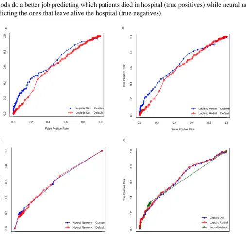
Figure 3 shows the ROC curves for each method using the default parameters and the optimized parameters. The best parameters found for each method are presented in Table 4.

Table 4 Performance metrics on test set using optimized parameters

Method Parameters KS TP TN FP FN Precision Recall Accuracy Logistic Dot C=0.01 0.21069 125 220 256 42 0.33 0.75 0.54 Logistic Radial Gamma=0.001, C=7 0.21689 120 234 242 47 0.33 0.72 0.55 Neural Network Learning Rate=0.3,

momentum=0.9 0.21737 57 417 59 110 0.49 0.34 0.74

Result shows that there is not a significant difference between the F-Measure of all methods; improving the results obtained by these methods on the baseline presented in the previous section.

Table 4 shows the performance metrics for each method using the optimized parameters, considering that the data set used for this test was composed by 476 patients that left hospital alive and 167 that passed in hospital, logistic regression methods do a better job predicting which patients died in hospital (true positives) while neural networks do a better job predicting the ones that leave alive the hospital (true negatives).

Fig. 3 Improvements for (a) Logistic Regression-Dot kernel (b) Logistic Regression-Radial kernel. (c) Artificial Neural Network.

0.0 0.2 0.4 0.6 0.8 1.0 0 .0 0 .2 0 .4 0 .6 0 .8 1 .0

False Positve Rate

T ru e P o s iti ve R a te

Logistic Dot Custom Logistic Dot Default

0.0 0.2 0.4 0.6 0.8 1.0 0 .0 0 .2 0. 4 0 .6 0. 8 1. 0

False Positve Rate

T rue P o si ti ve R a te

Logistic Radial Custom Logistic Radial Default

0.0 0.2 0.4 0.6 0.8 1.0 0 .0 0 .2 0. 4 0. 6 0. 8 1. 0

False Positve Rate

T ru e P o s itiv e R a te

Neural Network Custom Neural Network Default

a) b) c) 0.0 0.2 0.4 0.6 0.8 1.0 0 .0 0 .2 0 .4 0 .6 0 .8 1 .0

False Positve Rate

T ru e P o s itiv e R a te Logistic Dot Logistic Radial Neural Network d)

(8)

4.Conclusions and Future Work

This research compares four machine learning techniques used in medical data analysis and gave the parameters to extract a consistent data set of MIMIC II, so future researches can easily extract the same data and compare its result in a consistent way.

Our main finding is that, using three of the four methods analyzed in the paper, we were able to obtain similar results. These similarities suggest that a correct parameter calibration could be more important than method selection for this kind of analysis using this specific dataset.

The performance metrics (Table 2) shows that is possible to make relatively correct predictions using sparse data

and weakly correlated variables (column “Correlation with Dead” of Table 1). So with further investigation about the

parameters of each methods and the inclusion of new variables the methods could be refine to obtain better results. In particular, it is expected that the inclusion of the dimensions Maximum and Minimum (in this research only the average

was included) and new variables as “Arterial Blood Pressures” or “Temperature” could improve the models

performance.

References

1. Saeed, Mohammed, et al. "MIMIC II: a massive temporal ICU patient database to support research in intelligent patient monitoring." Computers in Cardiology, 2002. IEEE, 2002.

2. Zhang, Yang, et al. "Real-time clinical decision support system with data stream mining." BioMed Research International 2012 (2012). 3. Gerald, Lynn B., et al. "A decision tree for tuberculosis contact investigation." American journal of respiratory and critical care medicine

166.8 (2002): 1122-1127.

4. Thommandram, Anirudh, et al. "Classifying neonatal spells using real-time temporal analysis of physiological data streams: Algorithm

development.“ Point-of-Care Healthcare Technologies (PHT), 2013 IEEE. IEEE, 2013.

5. Mao, Yi, et al. "Medical data mining for early deterioration warning in general hospital wards." Data Mining Workshops (ICDMW), 2011 IEEE 11th International Conference on. IEEE, 2011.

6. Lehman, Li-wei H., et al. "A physiological time series dynamics-based approach to patient monitoring and outcome prediction." Biomedical and Health Informatics, IEEE Journal of 19.3 (2015): 1068-1076.

7. Eftekhar, Behzad, et al. "Comparison of artificial neural network and logistic regression models for prediction of mortality in head trauma based on initial clinical data." BMC Medical Informatics and Decision Making 5.1 (2005): 1.

8. Khan, Javed, et al. "Classification and diagnostic prediction of cancers using gene expression profiling and artificial neural networks." Nature medicine 7.6 (2001): 673-679.

9. Walsh, Paul, et al. "An artificial neural network ensemble to predict disposition and length of stay in children presenting with bronchiolitis." European Journal of Emergency Medicine 11.5 (2004): 259-264.

10. Brameier, Markus, and Wolfgang Banzhaf. "A comparison of linear genetic programming and neural networks in medical data mining." Evolutionary Computation, IEEE Transactions on 5.1 (2001): 17-26.

11. Zimmerman, Jack E., et al. "Acute Physiology and Chronic Health Evaluation (APACHE) IV: hospital mortality assessment for today's critically ill patients." Critical care medicine 34.5 (2006): 1297-1310.

12. Herland, Matthew, Taghi M. Khoshgoftaar, and Randall Wald. "A review of data mining using big data in health informatics." Journal of Big Data 1.1 (2014): 1-35.