CRANFIELD UNIVERSITY
Ömer Faruk Eker
A Hybrid Prognostic Methodology and its Application to
Well-Controlled Engineering Systems
School of Aerospace, Transport and Manufacturing
IVHM Centre
PhD Thesis
Academic Year: 2014 - 2015
Supervisors:
Assoc Prof Fatih Camci
Prof Ian K. Jennions
January 2015
CRANFIELD UNIVERSITY
School of Aerospace, Transport and Manufacturing
IVHM Centre
PhD Thesis
Academic Year 2014 - 2015
Ömer Faruk Eker
A Hybrid Prognostic Methodology and its Application to
Well-Controlled Engineering Systems
Supervisors:
Assoc Prof Fatih Camci
Prof Ian K. Jennions
January 2015
© Cranfield University 2015. All rights reserved. No part of this
publication may be reproduced without the written permission of
Abstract
This thesis presents a novel hybrid prognostic methodology, integrating physics-based and data-driven prognostic models, to enhance the prognostic accuracy, robustness, and applicability. The presented prognostic methodology integrates the short-term predictions of a physics-based model with the longer term projection of a similarity-based data-driven model, to obtain remaining useful life estimations. The hybrid prognostic methodology has been applied on specific components of two different engineering systems, one which represents accelerated, and the other a nominal degradation process.
Clogged filter and fatigue crack propagation failure cases are selected as case studies. An experimental rig has been developed to investigate the accelerated clogging phenomena whereas the publicly available Virkler fatigue crack propagation dataset is chosen after an extensive literature search and dataset analysis. The filter clogging experimental rig is designed to obtain reproducible filter clogging data under different operational profiles. This data is thought to be a good benchmark dataset for prognostic models.
The performance of the presented methodology has been evaluated by comparing remaining useful life estimations obtained from both hybrid and individual prognostic models. This comparison has been based on the most recent prognostic evaluation metrics. The results show that the presented methodology improves accuracy, robustness and applicability. The work contained herein is therefore expected to contribute to scientific knowledge as well as industrial technology development.
Keywords:
Integrated Vehicle Health Management, Prognostics and Health Management, Condition Based Maintenance, Hybrid Prognostics, Physics-based Prognostics, Data-driven Prognostics, Similarity-Physics-based Prognostics, Filter Clogging Modelling, Fatigue Crack Growth Modelling.
Acknowledgements
I would like to express sincere gratitude to my supervisor Professor Fatih Camci, for all his help and guidance carrying out the work presented in this thesis. I would also like to extend my gratitude to my co-supervisor Professor Ian K. Jennions, providing specialist knowledge in fluid dynamics as well as the IVHM field. I am also grateful to Professor Andrew Starr for his valuable feedback who was the subject advisor to this project. I would also thank Professor Philip Irving for his collaboration in fatigue crack modelling studies.
I would like to acknowledge the full sponsorship and feedbacks for this project provided by the Cranfield University IVHM Centre and its industrial partners: The Boeing, Rolls-Royce, Meggitt, BAE Systems, Thales, Alstom, and the UK Ministry of Defence.
I would also like to thank to my colleagues in IVHM centre for all kinds of support and assistance. In particular, I would like to thank to Faisal Khan for technical discussions on all sorts of interesting engineering topics which indirectly helped on this thesis completion.
Finally, I would like to thank my parents, my brothers and sisters who have supported me at every stage.
Table of Contents
Abstract ... i
Acknowledgements ... iii
Table of Contents ... v
List of Figures ... vii
List of Tables ... ix
List of Abbreviations ... x
1 Introduction ... 13
1.1 Research Problem Definition ... 14
1.2 Research Aims & Objectives ... 15
1.3 Contributions ... 17
1.4 List of Publications ... 17
1.5 Thesis Layout ... 18
2 Literature Review ... 20
2.1 Integrated Vehicle Health Management ... 20
2.2 Maintenance Strategies Overview ... 21
2.2.1 Condition-Based Maintenance ... 24
2.3 Review of Prognostics Approaches ... 29
2.3.1 Data-Driven Models ... 30
2.3.2 Physics-Based Models ... 36
2.3.3 Knowledge-Based Models ... 39
2.3.4 Hybrid Models ... 42
2.3.5 Challenges in Prognostic Modelling ... 51
3 Data Selection & Data Collection ... 56
3.1 Case Study 1: Available Prognostic Datasets ... 56
3.1.1 Milling Dataset & Tool Wear Modelling ... 57
3.1.2 Bearing Dataset & Spall Progression Modelling ... 58
3.1.3 Li-Ion Battery Dataset & Capacity Modelling ... 60
3.1.4 Turbofan Engine Degradation Simulation Dataset ... 61
3.1.5 IGBT Aging Dataset & Package Failure Modelling ... 62
3.1.6 Virkler Dataset & Fatigue Crack Growth Modelling ... 63
3.1.7 Dataset Comparison & Selection ... 65
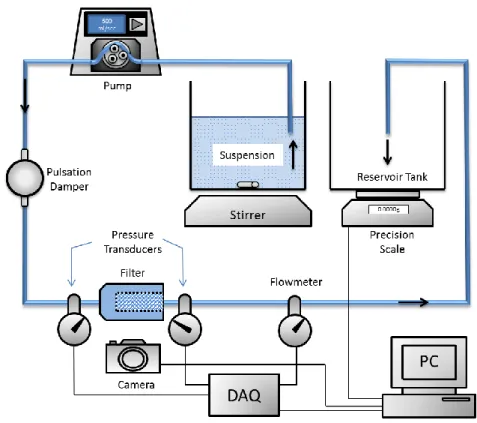
3.2 Case Study 2: Filter Clogging Data Collection ... 66
3.2.1 Test Rig Design & Setup ... 67
4 Methodology ... 85
4.1 Data-Driven Prognostic Modelling ... 85
4.1.1 Similarity-Based Prognostics ... 85
4.2 Physics-Based Prognostic Modelling ... 89
4.2.1 Particle Filters ... 90
4.2.2 Fatigue Crack Propagation Modelling ... 93
4.2.3 Filter Clogging Modelling ... 97
4.3 Hybrid Prognostic Modelling ... 110
4.3.1 Proposed Hybrid Prognostic Methodology ... 114
5 Results ... 117
5.1 Prognostic Performance Evaluation Metrics ... 117
5.1.1 Prognostic Horizon (PH) ... 119
5.1.2 α − λ Performance ... 120
5.1.3 Relative Accuracy (RA) ... 121
5.1.4 Convergence ... 121
5.2 Crack Propagation Modelling ... 122
5.3 Filter Clogging Modelling ... 136
5.4 Discussion ... 147
6 Conclusions & Future Work... 151
List of Figures
Figure 2.1 The OSA-CBM architecture ... 25
Figure 2.2. P-F curve of an equipment ... 25
Figure 2.3. Fault Diagnostics vs. Failure Prognostics in CBM ... 27
Figure 2.4. Prognostic and diagnostic phases ... 28
Figure 2.5. Prognostic models hierarchy ... 30
Figure 2.6. Hybrid prognostic model types ... 44
Figure 3.1. Virkler dataset visualisation ... 64
Figure 3.2. Filter clogging prognostic rig system design ... 68
Figure 3.3. PEEK particle size distribution ... 69
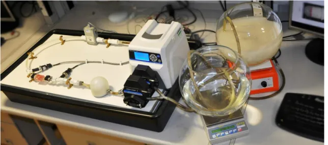
Figure 3.4. Filter clogging prognostic rig ... 70
Figure 3.5. Baldwin fuel filter ... 74
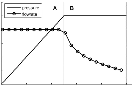
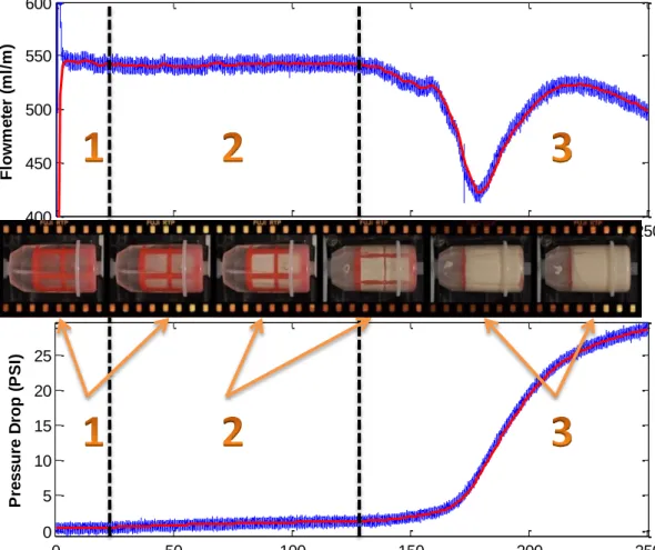
Figure 3.6. Pressure drop and flow rate measurements ... 74
Figure 3.7. Magnified pressure plot of a sample ... 75
Figure 3.8. Filtered and sampled complete dataset ... 76
Figure 3.9. The dataset and sieved particle relation ... 77
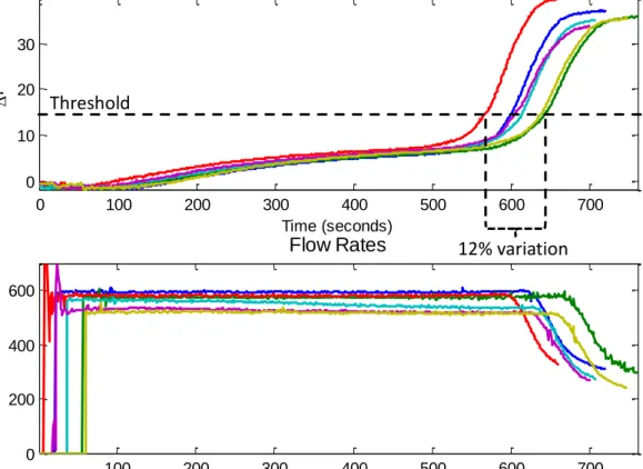
Figure 3.10. Initial data collection ... 79
Figure 3.11. Second attempt for data collection ... 80
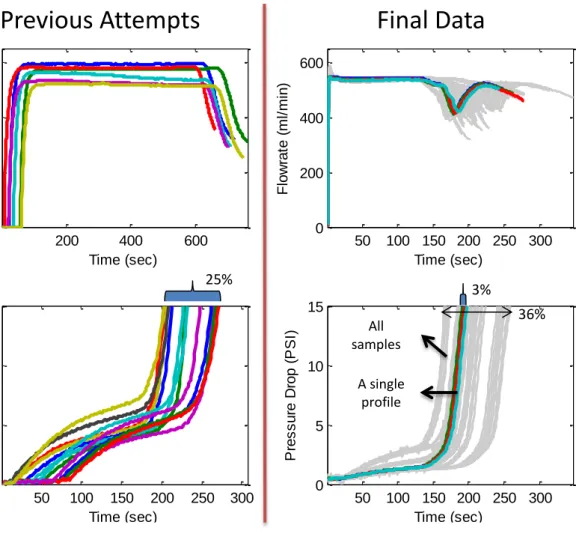
Figure 3.12. Pulsation dampening comparison ... 81
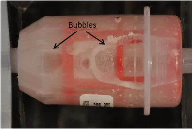
Figure 3.13. Accumulated bubbles inside the filter container ... 82
Figure 3.14. Improvements in pressure and flow rate values ... 83
Figure 4.1. Similarity-based prognostic RUL calculation ... 87
Figure 4.2. Schematic representation of cake build-up on filter medium .... 98
Figure 4.3. Constant rate vs. constant pressure filtration... 99
Figure 4.4. Filtration stages ... 100
Figure 4.5. Sphere packing simulation results of the adapted parameter . 106 Figure 4.6. Cake thickness calculation using filter images ... 108
Figure 4.7. Cake thickness modelling demonstration ... 109
Figure 4.8. Hybrid integration scenarios ... 112
Figure 4.9. Hybrid integration scheme demonstration ... 115
Figure 5.1. Hierarchical design of the prognostic metrics ... 118
Figure 5.2. Test specimen geometry ... 123
Figure 5.3. Paris Law and particle filter integration ... 124
Figure 5.4. System bias comparison ... 125
Figure 5.5. PbM vs DDM RUL visualisation on a Virkler dataset sample 126 Figure 5.6. RUL results for Virkler dataset scenario 3 ... 130
Figure 5.7. Performance results for Virkler dataset scenario 3 ... 131
Figure 5.9. Performance results for Virkler dataset scenario 4 ... 133
Figure 5.10. RUL results for Virkler dataset scenario 5 ... 134
Figure 5.11. Performance results for Virkler dataset scenario 5 ... 135
Figure 5.12. Original 100Hz vs 1Hz sampled data for filter clogging dataset ... 137
Figure 5.13. Final pressure drop trajectories for filter clogging dataset.... 138
Figure 5.14. Simulation results before Particle Filter integration ... 139
Figure 5.15. Cake thickness and pressure drop modelling ... 141
Figure 5.16. RUL results for filter clogging dataset scenario 3 ... 142
Figure 5.17. Performance results for filter clogging dataset scenario 3 ... 143
Figure 5.18. RUL results for filter clogging dataset scenario 4 ... 144
Figure 5.19. Performance results for filter clogging dataset scenario 4 ... 145
Figure 5.20. RUL results for filter clogging dataset scenario 5 ... 146
List of Tables
Table 2-1. Comparison of the benefits of prognostic approaches ... 43
Table 2-2. Hybrid prognostic model reference table ... 49
Table 3-1. Tool life and wear models ... 58
Table 3-2. Bearing fatigue life models ... 60
Table 3-3. Physics-based models for temperature cycling ... 63
Table 3-4.Prognostic approach applicability table ... 65
Table 3-5. Operational profiles ... 72
Table 3-6. Profile details of 45-53 μm particle size distribution ... 73
Table 3-7. Challenges & improvements ... 84
Table 5-1. Segment size construction for different scenarios ... 128
Table 5-2. Performance metrics comparison for crack propagation case study .. 148 Table 5-3. Performance metrics comparison for filter clogging case study 148
List of Abbreviations
AI Artificial Intelligence
ANFIS Adaptive Neuro-Fuzzy Inference System
ANN Artificial Neural Networks
ARIMA Auto-Regressive Integrated Moving-Average
ARMA Auto-Regressive Moving-Average
ASTM American Society for Testing and Materials
BBN Bayesian Belief Networks
BPNN Back Propagation Neural Networks
CBM Condition-Based Modelling
CDF Cumulative Density Function
CM Condition Monitoring
C-MAPSS Commercial Modular Aero-Propulsion System Simulation
CPNN Confidence Prediction Neural Networks
CRA Cumulative Relative Accuracy
DBN Dynamic Bayesian Networks
DDM Data-Driven Modelling
DP Damage Prognosis
DWNN Dynamic Wavelet Neural Networks
EKF Extended Kalman Filter
EoL End-of-Life
eUAV Electric Unmanned Aerial Vehicle
FFNN Feed Forward Neural Networks
FMECA Failure Mode, Effects, and Criticality Analysis
GM Gray Model
GPR Gaussian Process Regression
HHMM Hierarchical Hidden Markov Models
HMM Hidden Markov Models
HPC High Pressure Compressor
HSMM Hidden Semi Markov Models
HUMS Health and Usage Monitoring Systems
IGBT Insulated Gate Bipolar Transistor
ISHM Integrated System Health Management
IVHM Integrated Vehicle Health Management
KBM Knowledge-Based Modelling
KF Kalman Filters
kNN k-Nearest Neighbour
MAD Mean Absolute Deviation
MAPE Mean Absolute Percentage Error
MLE Maximum-Likelihood Estimation
MLP Multi-Layer Perceptron
MQE Minimum Quantisation Error
MSE Mean Squared Error
MTBF Mean Time Between Failures
MTTR Mean Time To Restore
NASA National Aeronautics and Space Administration
NDE Non-Destructive Evaluation
NI National Instruments
NN Neural Networks
nRMSE Normalized RMSE
OSA-CBM Open Systems Architecture for CBM
PbM Physics-Based Modelling
PCA Principle Component Analysis
PDF Probability Density Function
PEEK Poly-ether-ether-ketone
PF Particle Filters
PH Prognostic Horizon
PHM Prognostics and Health Management
PoF Physics of Failure
RA Relative Accuracy
RBF Radial Basis Function
RCM Reliability Centred Maintenance
RMSE Root Mean Squared Error
RNN Recurrent Neural Networks
RUL Remaining Useful Life
RVM Relevance Vector Machine
SBP Similarity Based Prognostics
SHM Structural Health Monitoring
SIR Sequential Importance Resampling
SOM Self-Organising Maps
SPC Statistical Process Control
SVM Support Vector Machines
SVR Support Vector Regression
TDNN Time Delay Neural Networks
TLFN Time Lagged Feed forward Networks
WAEP Weight Application to Exponential Parameters
Chapter 1
1
Introduction
This chapter briefly describes the basics of Integrated Vehicle Health Management (IVHM), a capability that enables a number of maintenance philosophies emphasizing prognostics, one of the most attractive research topics in this area. Also, the research problem found in the literature of engineering applications is discussed. Finally, the aims and objectives of this study are outlined and the PhD contribution is presented.
IVHM is a relatively new comprehensive technology, enabling many disciplines with an integrated framework. Maintenance strategies such as Condition Based Maintenance (CBM) or Reliability Centred Maintenance (RCM) are enabled using IVHM. Prognostics and diagnostics are integrated into the framework involving the monitoring of sensory information and predicting the future health level of the system, based on the monitored data. IVHM technology has potential applications in many fields such as aerospace, military systems, electronics, machinery, energy, and manufacturing. In IVHM, real-time sensory data obtained from the equipment is analysed continuously to detect and forecast the health states and to plan maintenance based on the forecasted health.
Prognostics is challenging and the fundamental technology within IVHM, where it requires identification of the current health level and extrapolating
it to a predefined failure threshold, concluded with the estimation of remaining useful life (RUL). The output of prognostics (i.e. RUL) is the duration between the current time and the time at which the forecasted health level reaches to a predefined threshold. Benefits of the prognostics motivate researchers and the industry to achieve reduced costs, increased safety and availability via better maintenance planning. In contrast with traditional maintenance philosophies, the IVHM approach enables modelling and tracking of individual equipment deterioration leading to a maintenance action only when it is necessary rather than performing scheduled maintenance. Note that, Prognostics and Health Management (PHM) is a relevant technology to IVHM where slight differences may appear which are reported in the in the literature. IVHM endeavours bringing a business model within the integrated scheme which is missing in the PHM. However, this research coverage involves both PHM and IVHM.
1.1
Research Problem Definition
Prognostics applications are relatively immature compared to diagnostics applications in the literature. Prognostic models can be categorised into two major categories. These are: 1) Physics-based models 2) Data-driven models. Physics-based models, also called model-based prognostics, consist of mathematical abstractions of a degradation path derived from first principles. They can be incorporated with Bayesian tracking methods (e.g. Particle Filters, Kalman Filters) in order to learn state of health parameters in the model and to cope with the sources of uncertainty (e.g. measurement noise) in measurement processes.
Alternatively, data-driven approaches employ historical run-to-failure data to construct a statistical or artificial intelligence based model aiming to accommodate the degradation process and predict the remaining useful life of the system. Extracted patterns from the signals, or raw data reflecting
the degradation pattern is used for predicting the time-to-failure with confidence bounds.
Approaches in both categories have their own advantages and disadvantages in real life applications. Data-driven models suffer from the inability to learn in portions of the operations where no such data exists. On the other side, physics-based models require high expertise in application field and tend to be computationally prohibitive to apply at system level. Approaches under both data-driven and physics-based categories require many conditions to be met. Besides, there is no universally accepted best model to perform prognostics due to variations on limitations of data availability, application constraints, and system complexity (Liao and Kottig, 2014). Furthermore, in real life applications, unmet requirements make the model imperfect, resulting in ineffective RUL predictions. Hence, a hybrid prognostic approach is aimed at leveraging the advantages of both approaches and to compensate for their limitations. In this research, these limitations and their effects are analysed in five different categories. The fifth scenario imitates the real world prognostic application limitations and presents an integration solution to enhance the prognostic applicability.
1.2
Research Aims & Objectives
The PhD aim is to develop a hybrid prognostic approach that integrates physics-based and data-driven prognostics in order to enhance the prognostic results and to increase the applicability of prognostics in real applications.
The core objectives of this research are:
To build an experimental rig with a high degree of accuracy, capable of taking data to validate prognostic algorithms.
To develop physics-based models (PbM) for the degrading components of two engineering systems.
To develop a data-driven model (DDM) for the degrading components of two engineering systems.
To develop an integration scheme for combining physics based and data driven prognostic approaches.
To investigate the applicability & performance of the hybrid model for the application scenarios mentioned.
The developed prognostic models (PbM, DDM, and Hybrid) have been implemented on two datasets: 1. Fatigue crack propagation dataset, 2. Filter clogging dataset. The former is a publicly available dataset, where a new experimental test rig has been designed and developed for the latter one. The experimental prognostic rig has been setup to produce a benchmark degradation dataset under different operational profiles. Variation under the same operation profile group is very low, whereas the spread in the complete dataset, consisting of all profiles, is significantly higher. On the other hand, the fatigue crack propagation dataset is a well-controlled set of crack growth experiments where the test specimens are exposed to a constant amplitude cyclic fatigue load. The dataset is publicly available and is known as the ‘Virkler Dataset’.
For the filter clogging experiment, a physics-based prognostic model is derived from the porous flow pressure drop equations to model the differential pressure in the system and predict future pressure levels. For the Virkler fatigue crack growth dataset, a physics-based model employing the Paris and Erdogan crack propagation formulation is used. The hybrid integration scheme is applied on both case studies. Performance and applicability analysis is conducted by investigating the prognostic outputs obtained from the two application scenarios. The outcome of the analysis helps in decision making on the level of integration in hybrid model. In addition, the development of a continuous learning environment that enhances the level of integration within product life cycle is studied.
1.3
Contributions
The intellectual contributions of this research are outlined below:
1. The development of a novel prognostic integration scheme enabling hybrid prognostic modelling to enhance prediction accuracy and robustness.
2. The collection of a prognostic benchmark dataset consisting of fifty six run-to-failure samples for filter clogging failure, obtained under sixteen different operational profiles.
3. A physics-based prognostic model of the clogging filter phenomena. 4. Introducing a new parameter to improve a data-driven prognostic
approach.
5. A literature survey and prognostic eligibility study on benchmark prognostic datasets available on the Internet.
1.4
List of Publications
A list of publications that contributes to the literature regarding this research is listed below:
Journal papers:
1. Eker, O.F., Camci, F., Jennions, I.K., “An Integration Scheme for Hybrid Prognostics”, IEEE Transactions on Reliability, to be submitted, Mar. 2015.
2. Eker, O.F., Camci, F., Jennions, I.K., “Physics-based Prognostic Modelling of Filter Clogging Phenomena”, Reliability Engineering and System Safety, submitted, Feb. 2015.
Conference Proceedings:
1. Eker, O.F., Skaf, Z., Camci, F., Jennions, I.K., “State-based Prognostics with State Duration information of Cracks in Structures”,
Proceedings of the 3rd International Conference in Through-life Engineering Systems, Volume 22, pp. 122-126, Nov. 2014.
2. Eker, O.F., Camci, F., Jennions, I.K., “A Similarity-Based Prognostics Approach for Remaining Useful Life Prediction”, Second European Conference of the Prognostics and Health Management Society, Nantes, France, 8-10 Jul. 2014.
3. Eker, O.F., Camci, F., Jennions, I.K., “Physics-based Degradation Modelling for Filter Clogging”, 2nd European Conference of the Prognostics and Health Management Society, Nantes, France, 8-10 Jul. 2014.
4. Eker O. F., Camci F., Jennions I.K., “Filter Clogging Data Collection for Prognostics”, Proceedings of the Annual Conference of the PHM Society 2013, New Orleans LA, USA, 14-17 Oct 2013.
5. Eker O. F., Camci F., Jennions I. K., “Major Challenges in Prognostics: Study on Benchmarking Prognostics Datasets”, 1st European Conference of the Prognostics and Health Management Society, Dresden, Germany, 3-6 July 2012.
1.5
Thesis Layout
Organisation of the thesis is as follows:
Chapter 2 introduces the maintenance technologies enabled by IVHM. A detailed prognostic literature survey consisting of the prognostic categorizations and comparisons of each category is presented.
Chapter 3 discusses publicly available prognostic datasets and the properties of each set with a comparison of prognostic eligibility analysis. Also, the details of filter clogging prognostic rig test design, setup, and data collection is presented.
Chapter 4 describes in detail the integration scheme for hybrid prognostic modelling. Data-driven and physics-based modelling methodologies are also discussed in this section.
Chapter 5 brings forward the prognostic results obtained from each methodology for different application scenarios. Prognostic performance analysis and results are given and a discussion section added in order to refer to the capabilities and imperfections of the proposed model.
Chapter 6 summarises the research presented in this thesis and the future work on this research is laid out.
Chapter 2
2
Literature Review
The primary aim of this chapter is to provide a detailed literature review regarding IVHM and Prognostics along with a review of maintenance strategies. The prognostics approaches are categorised and discussed in detail. Furthermore, an analysis on strengths and weaknesses of the approaches has been conducted for each class. This chapter is concluded with the prognostic modelling challenge analysis conducted by the researcher.
2.1
Integrated Vehicle Health Management
The Integrated Vehicle Health Management (IVHM) concept as introduced by NASA is defined as:
“… the capability to efficiently perform checkout, testing, and monitoring of space transportation vehicles, subsystems, and components before, during, and after operation(s)…must support fault-tolerant response including system/subsystem reconfiguration to prevent catastrophic failure; and IVHM must support the planning and scheduling of post-operational maintenance.” (NASA, Oct. 1992)
As mentioned in the above definition, IVHM acts an imperative role in aircraft operation management, and continues to offer the potential for a
paradigm shift in the way that aircraft organisations conduct business operations. Benedettini et al. (2009) postulate that IVHM is also potentially applicable to non-vehicle systems such as industrial process plants and power generation plants.
However, IVHM is not suitable for all manufactured assets due to the IVHM solution may be more expensive than the asset or service itself (Jennions, 2011). Therefore the technology is recommended to be applied for high-value complex products such as aircrafts, power generating equipment (e.g. wind turbines), or medical scanners.
Jennions (2011) documents the generic IVHM taxonomy consisting of following sub-categories:
Maintenance service offerings (e.g. CBM, Total Care, RCM) Business (e.g. Business models, IVHM mapping)
System design
Architecture
Analytics (e.g. Diagnostics, Prognostics)
Technologies (e.g. Structural Health Management (SHM))
IVHM enables many disciplines with an integrated framework. CBM, Health and Usage Monitoring Systems (HUMS), and RCM are some of the maintenance strategies offered under IVHM where diagnostics and prognostics considered under the analytics category. IVHM builds the background of this thesis along with the relevant technology, PHM.
Following sections present the maintenance strategies including CBM and its sub-disciplines which provide a basis for this research.
2.2
Maintenance Strategies Overview
Maintenance philosophies are classified into two categories, these are: 1. Reactive Maintenance (unplanned)
Corrective Maintenance
2. Proactive Maintenance (pre-planned)
Preventative Maintenance
Predictive Maintenance
From the historical perspective of maintenance, it can be stated that the most spectacular changes have occurred in the last sixty years following World War (Brown and Sondalini, 2014). Until then, corrective maintenance was the only option for a maintainer where equipment used to be fixed or replaced on a breakdown basis. Nevertheless, corrective maintenance is still in use for simple components such as light bulbs or a basic pipeline which are less risky and where the failure consequences are not fatal.
From the 1950’s, mechanisation and automation steps have risen due to the increasing intolerance of downtime and the significantly increasing cost of labour. Improved machinery was of lighter construction and ran at higher speeds provoking wear out more quickly which lead to the development of proactive maintenance.
Preventative maintenance is a sub-discipline of proactive maintenance in which the maintenance tasks are performed periodically. Periods are fixed intervals determined by using historical data (e.g. MTBF: Mean-Time-Between-Failures) and without any input from the individual equipment itself. Equipment is serviced on a routine schedule whether the service is actually needed or not. However, both reactive and blindly proactive (preventative maintenance) maintenance approaches have financial and safety implications associated with them. Routine inspection rounds and lubrication, bi-monthly bearing replacements, or maintenance inspections and overhauls on aircraft systems are some of the examples of preventative maintenance activities.
In the late 1970s, the effectiveness of conducting preventative maintenance started to be questioned. A common concern about ‘over-maintaining’ arose which led to the development of predictive maintenance. Adaptively determined scheduling of maintenance actions are the main features of predictive maintenance that distinguishes it from preventative maintenance. On the contrary, predictive maintenance is limited to those applications where the cost and consequences are critical and technically feasible (Pintelon and Parodi-Herz, 2008). Predictive maintenance is classified as two: Condition-based Maintenance (CBM) and Reliability-Centred Maintenance (RCM). RCM performs two tasks: first, analyse and categorise failure modes (e.g. FMEA) and second, assess the impact of maintenance schedules on system reliability (Kothamasu et al., 2006). RCM is based on manual inspections and basic data trending. CBM is discussed in further detail later in this chapter.
From the 1980’s systems became progressively more complex in nature, bringing a more competitive marketplace and intolerance of increased downtimes. As an example from the 21st century, Murthy et al. (2002) reports that the daily loss of revenue due to downtime is £320,000 for Boeing 747 aircraft. Increasingly, risk analysis and environmental safety issues have become paramount. New concepts such as condition monitoring and expert systems have emerged. The Institute of Asset Management has been established in the UK in mid-90’s which has been received significant attention from most organisations. In 2000’s, terms such as prognostics, IVHM, and integrated system health monitoring (ISHM) have emerged and taken place in literature gradually thus far.
To conclude, in engineering practices today, maintenance activities are predominantly intuitive and based on the expert’s or personnel’s experience that are familiar with the equipment. However, experience is becoming difficult to accumulate due to an ageing engineering workforce and improved asset reliability. In addition, when dealing with complex
equipment, human decision making is not always sufficiently reliable due to the multitude of interrelating failure modes (Sikorska et al., 2011). Industrial and military areas have become increasingly concerned about system availability and reliability, due to the fact that current systems became more complex and expensive which lead to an increase in competition drive more than ever. Maximised system availability and reliability, minimised failure and downtime cost are of great importance for many industries. Today’s sophisticated sensor technology enables engineers to track degradation processes and empowers for prognostic reasoning of equipment being monitored (Lee et al., 2006).
2.2.1 Condition-Based Maintenance
Condition-Based Maintenance (CBM) is a predictive maintenance strategy, whereby the maintenance tasks are performed when the need arises. The necessity concept is determined by assessing the health condition of the equipment continuously and extrapolating it to a predefined failure threshold (Camci and Chinnam, 2010; Eker et al., 2011).
The hierarchical steps of standardised Open Systems Architecture for Condition-Based Maintenance (CBM) are depicted in Figure 2.1. OSA-CBM is a layered approach, describing a standardised information delivery system in between its functional blocks. The process starts with acquisition of data and transmitting it to the higher level where the signal is processed (e.g. feature extraction). Third layer stands for diagnostics in which the comparisons are performed in order to detect and isolate different fault types (e.g. FMECA failure mode analysis). In the next level, the degradation level is identified to provide an input to prognostic block in order to be able to predict the remaining useful life of the asset. The top two layers are responsible for the intelligent decisions for a maintenance activity by means of the prognostic results and instrumentation, respectively.
An example of degradation in health level of an asset is shown in Figure 2.2. The P-F interval is the time interval between potential failure which is identified by health indicators, and an eventual functional failure. With CBM, it’s necessary that the P-F interval is long enough to enable corrective maintenance action to be taken (Jennions, 2011).
Figure 2.1 The OSA-CBM architecture
Figure 2.2. P-F curve of an equipment
Performing maintenance preparation when the system is up and running has a great effect on reducing the operation and support costs. In addition to the reduced down time, the inventory cost will be reduced as more time will be available for obtaining required parts. Moreover, the efficiency in logistics & supply chain will be increased by means of better preparation for
maintenance. Eventually, the life cycle cost of the equipment will be reduced, as they are used until the end of their lives.
2.2.1.1 Diagnostics and Prognostics in CBM
Diagnostics and prognostics are two of the major disciplines of CBM. In the literature, there is a minor disagreement that prognostics is related to and highly dependent upon diagnostics (Sikorska et al., 2011). Diagnostics involves detecting and reporting abnormalities in signal as well as identifying the fault type, and quantification of current health status of an asset, being the relatively mature area compared to prognostics. CBM with diagnostics outputs aims to stop and schedule a maintenance task for the system once an abnormality has been detected otherwise the system continues to operate. Once degradation is detected, unscheduled maintenance should be performed to prevent the failure consequences. It is not uncommon to spend more time in maintenance preparation than in performing the actual maintenance due to the lack of resources.
Ideally, in prognostics, maintenance preparation could be performed when the system is up and running, since the time-to-failure is known early enough. Thus, only the actual maintenance duration becomes the major contributor of the downtime which is way less than the fault diagnostic approach in CBM. As an example if prognostics can present a warning of a failure of an asset before 10 flight hours, re-test and installation steps can be pre-planned, yielding in saving of maintainer time and significant reduction in its variability (Hecht, 2006). Figure 2.3 illustrates the comparison of diagnostics and prognostics in CBM.
In general, incipient failures follow a progressive degradation path (Kwan et al., 2003). Detection of failure progression is more valuable compared to the detection of failure once it has reached to a severe point. Furthermore, it is a prerequisite for prognostics (Xiong et al., 2008). In other words, prognostic utilise the health severity or health status information transmitted from the
diagnostics base. Hecht (2006) states that prognostics for avionics is essential as the increasing of the number of complex systems comprising of electro-mechanical components in current and future aircrafts and a possible shortage of technicians capable of servicing them.
Figure 2.3. Fault Diagnostics vs. Failure Prognostics in CBM
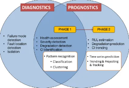
Prognostics involve two phases as shown in Figure 2.4. The goal of the first phase of prognostics is to assess the current health status. Severity detection, health assessment, and degradation identification are the terms used for describing this phase in the literature. This phase could also be considered under diagnostics as mentioned before. Usually, Bayesian filtering and/or pattern recognition techniques such as classification or clustering are employed in the health assessment part. The second phase, which is so-called the true prognostics, aims to predict the failure time by forecasting the degradation trend leading to the estimation of remaining useful life (RUL). Time series analysis, extrapolation, propagation, trending, projection and tracking are the terms used for describing this phase.
Prognostics imply forecasting of the system’s/component’s future health level by propagating the current health level until a failure threshold.
Consequently, it enables an ability to provide an estimate of the remaining useful life (RUL). Prognostics is considered to be one of the most challenging and key enabling technologies among the CBM steps (Zhang et al., 2006b; Peng et al., 2010; Daigle and Goebel, 2010).
Figure 2.4. Prognostic and diagnostic phases
2.2.1.2 Benefits of Prognostics with CBM
CBM approach has significant advantages on reducing the support and operating costs and leading to a more effective planning and operational decision making. An unexpected one-day stoppage in machinery industry may cost up to £160,000 (Peng et al., 2010). Another example from the return on investment for companies is the investment of £9,500 on monitoring the condition of systems prevents £315,000 of maintenance costs per year (Kothamasu et al., 2006).
In another example, FAA’s BRITE radar was maintained either with pre-arranged (proactive) or unscheduled (reactive) maintenance. Pre-pre-arranged maintenance decisions were taken reasonably before the potential failure utilising prognostics by monitoring of degradation in the radar. Unscheduled maintenance took seventeen hours higher than pre-arranged maintenance in mean time to restore (MTTR) which was fifteen times
higher than that of the pre-arranged maintenance in comparison (Hecht, 2006). A detailed review of prognostic approaches is presented in the following section.
2.3
Review of Prognostics Approaches
Amongst those papers reviewed, there is little consensus of prognostic field as to what categorisation is the most appropriate for prognostic models. In general, prognostic models can be categorised into four classes, these are:
1. Data-driven models 2. Physics-based models 3. Knowledge-based models 4. Hybrid models
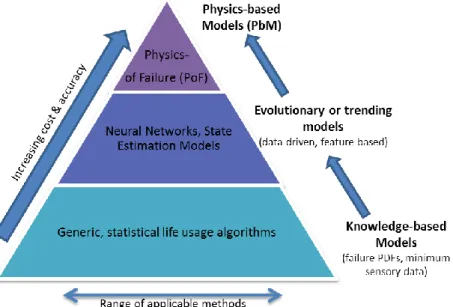
First three categories are illustrated in Figure 2.5, whereas a hybrid model implies fusion or combination of other methods is not shown in (Vachtsevanos et al., 2006) categorisation chart. This chart depicts the hierarchy of prognostic models based on the range of applicability, cost, and accuracy where knowledge-based models, being the most cost effective, find themselves a maximum applicability range in systems/components, albeit the accuracy of these models is less than the high accurate and costly physics-based models. Data-driven models fit in the middle of these models mentioned. Detailed discussion on comparison of the prognostic models will be presented in section 2.3.4.
Several literature surveys covering the prognostic models have been presented by (Liao and Kottig, 2014; Kothamasu et al., 2006; Lee et al., 2006; Zhang et al., 2006b; Peng et al., 2010; Vachtsevanos et al., 2006; Heng et al., 2009; Si et al., 2011; Luo et al., 2003b; Jardine et al., 2006). This literature review builds on the surveys referred in this section. In addition, current prognostic applications have emerged in the literature are further
discussed. In the following sections, a literature review of prognostic approaches within these categories is presented.
Figure 2.5. Prognostic models hierarchy (Vachtsevanos et al., 2006) 2.3.1 Data-Driven Models
Data-driven models (DDM) employ routinely collected condition monitoring data and/or historical event data instead of building a model based on system physics or human expertise. DDMs attempt to track the degradation of an asset using extrapolation or projection techniques (e.g. regression, exponential smoothing, and neural networks) or match similar patterns in the history of relevant samples to infer RUL (Liao and Kottig, 2014). They also rely on the past patterns of deterioration to forecast future degradation. Usually system or loading inputs are not involved in data driven prognostic modelling. Assumption for models in this category is that the future system inputs or operational profile remains constant or consistent with the past data. Since data-driven prognostics have no elaborate information (e.g. physical information) related to the asset or system, it is considered to be a black-box operation (Zhang et al., 2009). Data-driven models are divided into two categories: Statistical models and Artificial Intelligence-Based (i.e. machine learning) models.
2.3.1.1 Statistical Models
Statistical approaches construct models by fitting a probabilistic model to the data without depending on any engineering or physical principle. These approaches rely on statistical models and observed data to support the forecasting of the RUL of equipment. A comprehensive study on statistical data-driven models for remaining useful life estimation was conducted by Si et al. (2011). They divided statistical models into two categories based on the nature of condition monitoring (CM) data type used.
Typically, CM data can be divided into two categories: direct CM data, and indirect CM data. Direct CM data indicates the health level of system directly (e.g. crack size, wear level) whereas indirect CM reflects the underlying system health partially or indirectly (e.g. sensor information, vibration, oil based monitoring). Wiener and Gamma processes, regression-based models, and Markovian-regression-based models find place under the models based on direct CM data; whereas, Stochastic Filtering-Based Models, Covariate-Based Hazard Models, Hidden Markov Models (HMMs) and, Hidden Semi Markov Models (HSMMs) are under the indirect CM category. Brownian Motion (or Wiener Processes) are a continuous state prognostics data driven models and their probability density function (PDF) is considered to be inverse Gaussian distribution. Wiener Processes use only the current health status instead of using past event data. Wang and Carr (2010) proposed an improved version of Brownian motion-based stochastic degradation model for remaining useful life prediction of monitored plants. They contributed to the literature in two ways: Firstly, drifting the parameters of Brownian motion model by using Kalman Filters. Secondly, they used failure distribution threshold instead of using a constant threshold.
Gamma process is known for its simplicity. It’s a special version of Markovian-Based processes with continuous state representation (Si et al.,
2011). A Gamma process-based deterioration model on (Hudak et al., 1978) crack growth data was implemented by Lawless and Crowder (2004). They incorporated covariates and a random effect to characterise the different rates among the different individuals.
Bunks et al. (2000), Camci (2005), Baruah and Chinnam (2005) referred that the HMM based models could be applied in the field of prognostics in machining processes. Zhang et al. (2005) have investigated the use of Hidden Markov Models (HMMs) in bearing fault prognosis. They applied a combination of Principle Component Analysis (PCA) and HMM in order to obtain the degradation index of bearings, and they implemented Li et al.'s (2000) stochastic defect propagation model for predicting the RUL’s of components.
Marjanovic et al. (2011) presented a combination of Auto-Regressive Moving-Average (ARMA) & hypothesis testing and HMMs on a steam separator subsystem of thermal plants. However, both techniques provide inaccurate RUL results. They accounted for the problem as the methods were not taking into consideration of system’s current state. They supplied prognostics results with a literature review. Auto-Regressive Integrated Moving-Average (ARIMA) models are an extended version classic ARMA models, enabling to model non-stationary time series signals. Typical ARMA models found to be less reliable for long-term predictions (Liao and Kottig, 2014). Examples of ARIMA model in prognostic application is found in (Wei Wu et al., 2007; Saha et al., 2009)
Camci (2005) developed an integrated diagnostics and prognostics methodology that employ support vector machines (SVM) and HMMs. Camci and Chinnam (2010) compared the results of HMMs and Hierarchical Hidden Markov Models (HHMMs) on a CNC drilling machine degradation dataset, reporting that the proposed model, HHMM, outperform regular HMMs in the literature. Another application of HMMs
in prognostics can be found in (Medjaher et al., 2012) in which they present a Gaussian Hidden Markov Models represented by Dynamic Bayesian Networks (DBN) for bearings.
As an extension to SVMs, the Support Vector Regression (SVR) models are highly capable of addressing regression problems especially in cases where data is sparse (Khawaja, 2011). Applications of SVR on pattern recognition and prediction problems can be found in (Zhang et al., 2006a; Thissen et al., 2003; Mattera and Haykin, 1999).
Dong et al. (2006), Dong and He (2007b) Dong and He (2007a) proposed several Hidden Semi-Markov Model (HSMM) fault classification and prognostics applications on UH-60A Blackhawk main transmission planetary carriers in which HSMMs generate a segment of observations and estimate the durations from training data unlike HMMs which generate single observation for each state. Examples of discrete state-based approach for prognostic approaches can be found in (Eker et al., 2011; Eker and Camci, 2012; Guclu et al., 2010a).
Proportional Hazard Model and Proportional Intensity Model (PIM) are also useful approaches for RUL estimation in combination with a trending model for the fault propagation process. Cox (1972) introduced the proportional hazard model to estimate the influences of diverse covariates affecting the RUL of a system. RUL prediction for a Markov failure time process which involves a joint model of hazard model and Markov property for covariate evolution as a special case has been discussed by (Banjevic and Jardine, 2006). Another hazard rate algorithm was developed by (Li et al., 2007) to extract the repeated failure indications. A proportional hazard model for catastrophic failures and multiple degradation features of single equipment was introduced by (Liao et al., 2005).
intervals: First, the installation–potential failure (I-P); second, potential failure-functional failure (P-F).
Sheppard and Kaufman (2005) proposed a prognostics approach using Dynamic Bayesian Network (DBN) to model the changes over time. Bayesian Belief Networks (BBN) is recommended by (Przytula and Choi, 2007) for prognostic purposes, since the estimation of RUL can be done within the framework of BBNs.
Lastly, similarity-based prognostic approaches are usually effective when large amounts of historical data are available where a similarity matrix in between the current and historical data contributes to the estimation of RUL. Examples of Similarity-based Models for prognostics can be found in (Wegerich, 2004; Zio and Di Maio, 2010; Wang et al., 2008; Cheng and Pecht, 2007; Cheng and Pecht, 2007; Liu et al., 2007). Note that, some of the similarity-based approaches are categorised under the knowledge-based prognostic approaches (Wang, 2010). Details of the similarity based modelling approach are discussed in Chapter 0.
2.3.1.2 Artificial Intelligence-Based Models
Artificial Intelligence (AI) based or machine learning models attempt to recognise complex patterns and make intelligent decisions based on the empirical data. Machine learning approaches are adaptable to the situations where problem solutions require knowledge that is difficult to specify however enough data or observations are available. Artificial Neural Networks (ANN), Self-Organising Maps (SOM), and decision trees are common examples of machine learning approaches to be used for supporting the detection and diagnostics as well as prediction processes.
ANNs are perhaps the most commonly used machine learning techniques for prognostics; consisting of input, hidden, and output layers that interact with each other with numerically weighted connections inspired by the
neural structure of the human brain. ANNs are as multi-input-multi-output nonlinear blackbox function approximators, categorised into two classes; these are, supervised and unsupervised learning. The supervised learning models employ input data (i.e. sensor information, condition monitoring data) and target data (i.e. direct health indicators, health state) in order to train the weights and learn the complex patterns. The unsupervised learning models adapt to find hidden structure in the unlabelled data. Clustering algorithms (e.g. k-means clustering, SOM) are examples of unsupervised learning algorithms. Eker et al. (2011) used k-means clustering algorithm along with Calinski-Harabasz clustering evaluation index for the health state identification of railway turnout mechanisms, whereas the RUL prediction part is carried out by means of a state-based prognostic algorithm they developed.
Back propagation (BP) neural networks is a type of ANN, was utilised with a grey model in (Dong et al., 2004) for predicting the machine health condition. Gebraeel and Lawley (2008) proposed a degradation model based on dynamic wavelet neural networks (DWNN) in which the condition monitoring data was employed to estimate the RUL of partially degraded assets. Another example of DWNN in prognostics can be found in (Vachtsevanos and Wang, 2001). Huang et al. (2007) applied quantisation error indicator method (i.e. a derivation of SOM network) to assess the ball bearing degradation process and predict the remaining life. Time Delay Neural Networks (TDNN) is used for forecasting of a railway turnout systems in (Yilboga et al., 2010). A multi-layer perceptron NN along with regression NN is employed in (Herzog et al., 2009) for estimation through two application scenario. Ak et al. (2013) integrated a genetic algorithm to train ANN for predicting wind power under high uncertainty conditions. Mahamad et al. (2010) used Feed-Forward Neural Networks (FFNN) to predict RUL for a bearing failure case study.
Recurrent Neural Networks (RNN) with feedback connections can be considered as a non-linear extended version of classical ARMA models (Wang et al., 2004). RNNs have an advantage over generalised FFNNs where the uncertainty presentation of predictions is more robust. Zemouri et al. (2003) used recurrent radial basis neural networks to dynamically detect breakdowns and predict time series of nonlinear system states of gas ovens. Other examples for Recurrent Neural Networks for predicting machine condition trend can be found in (Yam et al., 2001; Heimes, 2008; Zhigang Tian, 2009). In the next section, literature review of physics-based models is provided.
2.3.2 Physics-Based Models
Physics-based models (PbM), also called ‘based Prognostics or Model-based Approaches’, typically involve describing the physics of the equipment and the failure mechanism. The author prefers to use the term ‘physics-based models’ rather than ‘model-‘physics-based prognostics’ since the most data-driven approaches use models as well. This way of categorization gives a better ability to distinguish physics-based and data-driven models (Daigle, 2014).
In PbMs, mathematical models of failure are usually employed which is directly tied to health degradation. In order to provide knowledge rich prognostics output; PbMs are attempted to combine defect growth formulas, system specific mechanistic knowledge and condition monitoring data. These models assume that an accurate mathematical model for component degradation can be constructed from first principles. Residuals, the outcomes of consistency checks between sensor measurements and mathematical model outputs, are utilised as features of health condition in PbM approaches. Thresholds to detect the presence of faults are determined by using statistical techniques. In addition, model parameters are identified using empirical data obtained from specifically designed experiments (Liao
and Kottig, 2014). Physics-Based Models are implemented in three different ways (Sikorska et al., 2011); firstly, dynamic ordinary or partial differential equations that can be solved with approximation approaches (e.g. Lagrangian or Hamiltonian dynamics), secondly, state-space methods (i.e. no differential equations), thirdly, simulation methods.
Kacprzynski et al. (2002) employed a physical stochastic model on gears. They calibrated the parameters for physical stochastic prognostics & diagnostics using system level features extracted from test specimens. Byington et al. (2004b) developed a fault detection and prediction algorithm for flight actuators which applies parametric identification and physical modelling techniques. Cempel et al. (1997) and Qiu et al. (2002) applied physics-based approaches to prognostics which have involved deriving the explicit relationship between condition variables and the current lifetime and failure lifetime via mechanistic modelling. Both of them applied their model for energy processors and bearings by employing vibration sensor measurements respectively. A general method for tracking the progress of a hidden damage process was proposed by (Chelidze and Cusumano, 2004). The proposed model is applicable for a given situation where a slowly evolving damage process is connected to a fast, directly observable dynamic system. Kacprzynski et al. (2004) fused diagnostic information and physics of failure modelling and applied for helicopter gear prognostics. A hierarchical modelling approach proposed by (Lesieutre et al., 1997) for system simulation to determine remaining useful life.
A physics-of-failure approach reinforced with Kalman filters were used to track the dynamics of the frequency of accelerometer sensor signals in tensioned steel band by (Swanson, 2001). Phelps et al. (2001) used a Kalman Filter with an associated interacting multiple model to perform tracking of sensor-level test-failure probability vectors for prognostics. Assumptions for Kalman Filters are that the system exhibits a linear process and the noise in the system follows Gaussian distribution. Extended Kalman Filters and
Unscented Kalman Filters are some of the extensions to the traditional Kalman Filters in which the system is not bounded by the linear process. Hu et al. (2012) presented an Extended Kalman Filter approach for estimation of Lithium-ion battery life. Particle filters are a generic type of Bayesian tracking methods used with physics laws (i.e. in the form of differential equations) in which the model is not bounded by the assumption of linearity in the system and Gaussian noise. Instead of using deterministic probability distributions, significant numbers of particles are employed representing the health state of the system distribution. A number of examples are available in prognostic modelling literature for particle filters (Daigle and Goebel, 2010; Zio and Peloni, 2011; An et al., 2013). Detailed discussion of particle filters is given in section 4.2.1.
Crack growth modelling is a widely used physics-based approach. Paris & Erdogan Law (Paris and Erdogan, 1963) is being used in several physics-based prognostics applications. Li et al. (2000) and Li et al. (1999) correlated defect growth rate of rolling element bearings to the material constants (i.e. C and m) and to defect area size based on Paris & Erdogan’s law. They tuned both their defect diagnostic and defect propagation model parameters by monitoring of the system signals. Luo et al. (2003b) described an integrated prognostic process based on model-based simulation data under nominal and degraded conditions. Forman law of linear elastic fracture mechanics was used by (Oppenheimer and Loparo, 2002) in order to model rotor shaft crack propagation. Orsagh et al. (2003) and Orsagh et al. (2004) employed a version of the Yu-Harris life equation for estimating the spall initiation. They used Kotzalas-Harris spall progression model to forecast the time to failure. Paris & Erdogan Law is also used in (Li and Choi, 2002; Li and Lee, 2005) to model gear crack growth. Most of the crack growth prediction models mentioned here are assumed that defect area size can be estimated using vibration data as the defect area size measurements are usually not available without interrupting the machine condition. A
comprehensive case study on modelling of fatigue crack propagation is provided in section 4.2.2.
Physics-based models are considered to be more accurate if an accurate mathematical model representing the degradation process is fitted in the model thoroughly (Liao and Kottig, 2014). And the requirement concept on the data is significantly less, compared to the data-driven models. However, PbMs are usually component or system specific models which mean usually they cannot be applied to other type of components or systems in which the physics of failure mechanism is different. Another disadvantage is that the PbMs are costly compared to other approaches whereas they are the most suitable approach for cost-justified applications where accuracy weighs most other factors (Heng et al., 2009).
2.3.3 Knowledge-Based Models
It is usually difficult to obtain an accurate mathematical model in real-world applications which limits the use of physics-based prognostic models. Due to the absence of a complex model, systems tend to be maintained with simpler models such as knowledge-based models (KbM). Knowledge or experience-based prognostic approaches are the simplest way of performing prognostics where the statistical historical failure information of systems is utilised for predicting the RUL (Vachtsevanos et al., 2006). The use of knowledge-based models is automated representation of how a human domain expert solves a problem (Liao and Kottig, 2014). Expert systems and fuzzy logic are two generic examples of these models.
Disadvantages of knowledge based systems can be listed as: Hard to obtain domain knowledge and extract rules
Handling of new situations which are not stored in knowledge base is limited
Computational difficulty increases dramatically as the number of rules increases (i.e. combinational explosion problem)
No confidence limits are supplied 2.3.3.1 Expert Systems
Expert systems have been used since 1960s, and are considered as an artificial intelligence (AI) program that represent domain expert knowledge in solving a problem related to a particular domain. In expert systems, knowledge of domain experts is stored in the knowledge base where the extracted rules are applied into the failure situations by the maintainer. Knowledge-based rules are generated from collections of real experiments. Basic IF-THEN statement rules are often based on heuristic facts acquired by experts over a number of years (Sikorska et al., 2011). Outputs of expert systems are singular rather than a distribution of RUL.
Expert systems have traditionally been used in failure diagnostics cases and it has started to be implemented in prognostics applications as well. Lembessis et al. (1989) developed an online expert system called CASSANDRA, which was built to monitor the condition of industrial equipment with the intent of fault prognostics.
Biagetti and Sciubba (2004) developed an expert system called PROMISE (Prognostics and Intelligent Monitoring Expert System) which carries out both diagnostic and prognostic duties and provides solutions to system maintenance in plants. However no RUL information was provided with their proposed method.
Butler (1996) developed an expert system based framework called FDPM (Failure Detection and Predictive Maintenance) which consists of several expert-system-related databases and components. It was applied on a power distribution system component for predicting maintenance demands.
2.3.3.2 Fuzzy Logic
Similar to expert systems, fuzzy logic is a problem solving mechanism providing a robust mathematical framework to deal with non-statistical uncertainty and real world imprecision. A fuzzy system consists of a knowledge base; fuzzy rule, and the implementation algorithms for applying the logic. Fuzzy logic has a wide application area from simple small components to large workstations. Unlike expert systems, the fuzzy logic system has the ability to model system behaviours in continuum mathematics of fuzzy sets rather than with traditional discrete values. Fuzzy logic systems are usually incorporated with other methodologies such as neural networks (NN) or expert systems.
Choi et al. (1995) proposed a fuzzy expert system called ‘Alarm Filtering’ and Diagnostic System (AFDS) which provide clean alarm pictures and system wide failure information during abnormal states. And also providing alarm prognosis to notify the operator of process abnormalities.
Dmitry and Dmitry (2004) presented a fuzzy logic process in which the input data is mapped into fuzzy variables (i.e. fuzzification) using membership functions and de-mapping the fuzzy variables processed into numerically precise outputs (i.e. defuzzification). This methodology has been used widely in control applications such as in (Lee, 1990).
Feng et al. (1998) proposed a dynamic fuzzy system for real-time condition monitoring and incident prevention. However, the RUL was not calculated whereas the applicability of fuzzy logic into prognostics was demonstrated. A comparison of a fuzzy logic model and neural networks is conducted by (Majidian and Saidi, 2007) for predicting the life of boiler tubes. Results show that neural network performed better where the applicability of NNs was favourable compared to the fuzzy logic model.
Unlike Majidian and Saidi's (2007) work, fuzzy logic is usually integrated in RUL calculation as an auxiliary method for the primary method to enhance prediction results. Fuzzy logic has an ability of dealing with incomplete or imprecise input information with the use of linguistic variables such as ‘low’, ‘very low’, which provides an intuitive way of reasoning and representing of failure health level. On the other hand; having no memory, limited capability of learning, and difficulties of determining good fuzzy rules and membership functions are some of the disadvantages of fuzzy logic.
2.3.4 Hybrid Models
It has been found to be difficult to predict the trends of all characteristic parameters by using an individual prognostic approach since the parameters are diversified in real world cases (Peng et al., 2010). The prognostic models under hybrid category combine multiple prognostic approaches in order to leverage the strengths of prognostic methods leading to enhanced prognostic results. Combination, fusion, integration, and hybrid terms are used for prognostic approaches in the literature for hybrid prognostic approaches. It is relatively a new area in prognostics and offers a promising concept for prognostics.
Hybrid prognostic approaches consist of several advantages, some of these are:
Imperfections of individual approaches will be compensated; furthermore, merits of them could be utilised;
Prediction accuracy; hence prognostics performance can be enhanced; Computation complexity may be reduced.
Summarisation of advantages and disadvantages of prognostic approaches are shown in Table 2-1. A highly detailed comparison of prognostic models from an industrial point of view can be found in (Sikorska et al., 2011).
Table 2-1. Comparison of the benefits of prognostic approaches
Advantages Disadvantages Physics-Based Models Accurate compared to other
approaches (if a good representative of mathematical model is available)
Higher precision
Requires less data compared to other approaches
Suitable for creation in design phase
Difficult to create a model especially for complex systems
Sensitive to the design and material properties Sufficient component
information and a good insight of the failure mechanism is required High cost of implementation Component or system specific Data-Driven Models Easy to conduct & simplicity
in implementation Flexible and adaptable Suitable to all levels
(component, system) More robust to changes in
material or design
compared to physics based Low cost
Need data representing the failure progression, which is often not possible to obtain Computational complexity may
be high
Difficulty in determining of the failure thresholds
Knowledge-Based Models
Simple and easy to understand No model is required Wide application area and
lower cost
Ability of dealing with incomplete, noisy or imprecise input information
Not always easy to obtain domain knowledge and extract rules
Handling of new situations which are not stored in knowledge base is limited Computational difficulty
increases dramatically as the number of rules increases
Limited capability of learning No confidence limits are
provided
Liao and Kottig (2014) have conducted an extensive research on hybrid prognostic model categorisation. According to their study, hybrid models are classified into five different categories as shown in Figure 2.6 where:
Knowledge-Based Model + Data-Driven Model (H1)
Knowledge-Based Model + Physics-Based Model (H2)
Data-Driven Model + Data-Driven Model (H3) Data-Driven Model + Physics-Based Model (H4)
Knowledge-Based Model + Data-Driven Model + Physics-Based Model
(H5)
Figure 2.6. Hybrid prognostic model types (Liao and Kottig, 2014)
2.3.4.1 Knowledge-Based Model & Data-Driven Model
Hybrid prognostic models under this category represent incorporation of expert systems or fuzzy logic systems along with data-driven approaches. These approaches can add the flexibility of integrating domain knowledge into data-driven models for health state estimation where the RUL calculation is performed by a data-driven model.
Artificial Neural Networks (ANN) is usually incorporated with expert systems or fuzzy logic systems. Brotherton et al. (2000) applied a neurofuzzy (NN & FL) combination method on gas turbine engines. NN learning procedures are combined with fuzzy interference system linguistic