Bayesian survival analysis using gene expression

(1)

Bayesian Survival Analysis Using Gene Expression

A THESIS SUBMITTED TO

THE SCHOOL OF MATHEMATICAL SCIENCES SCIENCE AND ENGINEERING FACULTY OF QUEENSLAND UNIVERSITY OFTECHNOLOGY

BRISBANE, QUEENSLAND, AUSTRALIA

IN FULFILMENT OF THE REQUIREMENTS FOR THE DEGREE OF DOCTOR OF PHILOSOPHY

Sri Astuti Thamrin

School of Mathematical Sciences

Science and Engineering Faculty Queensland University of Technology

Brisbane, Queensland, Australia

(2)

(3)

Bayesian Survival Analysis Using Gene Expression

A THESIS SUBMITTED TO

THE SCHOOL OF MATHEMATICAL SCIENCES SCIENCE AND ENGINEERING FACULTY OF QUEENSLAND UNIVERSITY OFTECHNOLOGY

BRISBANE, QUEENSLAND, AUSTRALIA

IN FULFILMENT OF THE REQUIREMENTS FOR THE DEGREE OF DOCTOR OF PHILOSOPHY

Sri Astuti Thamrin

Supervisor: Professor Kerrie L. Mengersen Associate Supervisor: Dr James M. McGree

Statistical Science

School of Mathematical Sciences

Science and Engineering Faculty Queensland University of Technology

Brisbane, Queensland, Australia

(4)

(5)

Copyright in Relation to This Thesis c

(6)

The work contained in this thesis has not been previously submitted to meet require-ments for an award at this or any other higher education institution. To the best of

my knowledge and belief, the thesis contains no material previously published or written by another person except where due reference is made.

Signature:

Sri Astuti Thamrin

oS /

o5

_/*otz

1V

(7)

Dedicated to Mama, Ayah

Setiawan, Nafis and Tsaniya.

(8)

(9)

Abstract

This research aims to compare and apply Bayesian models for patient survival using gene expression as explanatory variables. Three models were examined; the

Weibull model, the Weibull mixture model and the Weibull cure model. Bayesian model averaging (BMA) was developed to produce better descriptions of genetic

contributors to survival and of subgroups of patients with different survival charac-teristics. This can in turn provide insight into improved treatment regimes for these

patients.

In the development of the methodology, some important issues such as the effect of censored data were addressed. This research indicates that censoring has an

effect on the performance of the Weibull mixture models in that as the proportion of censoring increases, poorer parameter estimates were obtained in terms of both bias

and precision. Censoring also had a different effect on estimating the parameters of the mixture model, depending on the “closeness” of the components.

The application of BMA to combine the three competing models produced more

robust predictions of survival time. BMA also allowed the identification and analy-sis of more detailed relationships between gene expression in given phenotypes and

the survival times of the patients.

(10)

(11)

Keywords

Bayesian, Gene expression, Diffuse large B-cell lymphoma, Survival analysis, Model comparison, Variable selection, Sensitivity analysis, Bayesian modelling, Right

censored data, Mixture model, Weibull distribution, Markov Chain Monte Carlo, Bayesian model averaging, Cure model.

(12)

(13)

Acknowledgments

First and foremost, I offer my humble thank to Allah SWT for giving me the opportunity, strength and guidance to undertake my PhD.

This work would not have been possible without the support and help of many

people. I would like to convey my gratitude to my supervisors Prof. Kerrie Mengersen and Dr. James McGree for their supervision, unflinching encouragement, advice,

and guidance to perform this research. Without their help, I would not have been able to finish my study. Words is not enough to express how grateful I am. Kerrie,

I really appreciate the effort you put in helping and guiding me throughout my study, although sometimes I need time to catch your ideas. Thank you James, for

your assistance, discussion, mentoring, and patience with my questions. Again, my sincere thank you for both of you.

I would like to acknowledge the Minister of Education and Cultural of

Indone-sia, Directorate of General of Higher Education (DGHE)/DIKTI and Hasanuddin University for their financial support which made this research possible.

I would like to thank to my colleagues at QUT and Bayesian Research and

Application Group (BRAG), specially Dr. Nicole White, Su Yun Kang, James McKeon, Dr. Xiaodong, Darssan and Ben for their help, support and beautiful

friendship.

Next, I have to praise the patience and perseverance of my adored husband, Setiawan Aswad who has accompanied me and taken care of our beloved son and

(14)

I would not be a very different person today, and it would have been certainly much harder to finish my PhD.

I also would like to thank to my friends from Indonesia in Brisbane, especially

Sapri Pamulu family, Raja Juli Antoni family, Isnani Dzuhrina, Anak Agung Diah Parami Dewi and Gusti Dharmayanti and other members of Indonesian

Communi-ties in Brisbane. They certainly have genuinely helped and supported me and my family in many ways, helping to make my study and our lives easier.

Last in this list but first in my heart, I would like to thank to my family members

in Indonesia in particular my mother and father, my grandmother, my brothers, my mother and father in law for their constant emotional support and encouragement.

This PhD is an answer of my father’s challenge to study higher than him.

“Whoever struggles will achieve the goal, whoever follow patience will be suc-cessful”.

(15)

5 The Impact of Censored Survival Data on Bayesian Analysis when Fit-ting A Mixture of Weibull Models 77 5.1 Abstract . . . 79 5.2 Introduction . . . 79 5.3 Methods . . . 81 5.3.1 Model formulation . . . 81 5.3.2 Computational Method . . . 84 5.3.3 Model Evaluation . . . 85 5.3.4 Simulation study . . . 86 5.4 Results . . . 87 xv

(18)

5.4.2 Application Using Real Data . . . 97

6 Modelling Survival Data to Account for Model Uncertainty: A Single Model or Model Averaging? 105 6.1 Abstract . . . 107

6.2 Introduction . . . 107

6.3 Methods . . . 109

6.4 Models . . . 112

6.4.1 Weibull Model . . . 112

6.4.2 Weibull Mixture Model . . . 115

6.4.3 Cure Model . . . 117

6.5 Application Using Real Data . . . 120

6.5.1 DLBCL Dataset . . . 120

6.5.2 Results . . . 121

7 Conclusions and Future Work 133 7.1 General discussion . . . 133

7.2 Future work . . . 138

References 162

(19)

List of Figures

2.1 Gene structure and protein synthesis . . . 9

3.1 Weibull failure distribution with differing parameter values. . . 28

3.2 Weibull densities with different values of the shape parameter. . . . 28

4.1 Posterior densities ofαandλusing Weibull survival model without

covariates for DLBCL data. . . 66

4.2 Posterior estimated survivor function S(t) with 95% credible

in-terval for DLBCL data. Graph a) without covariates and b) with covariates (GC-B signature 2.24, lymph node signature 0.43, BMP6

signature -0.22 and MHC class II signature 1.35) . . . 67

4.3 The graph for observed survival time versus the expected survival time for training dataset (a) and validation dataset (b). . . 69

4.4 Posterior predicted survival functionS(t)of four different patients

for DLBCL data with covariates after chemotherapy. . . 71

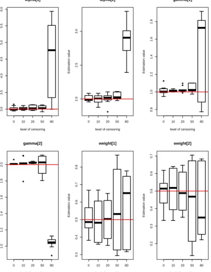
5.1 Box-plots of posterior estimates of parameters (α,γ,π) for model

M1 with five different levels of censoring. . . 88

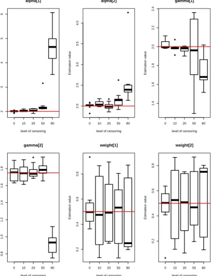
5.2 Box-plots of posterior estimates of parameters (α,γ,π) for model M2 with five different levels of censoring. . . 89

(20)

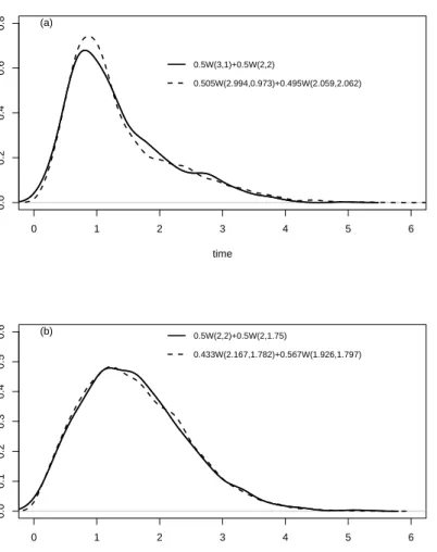
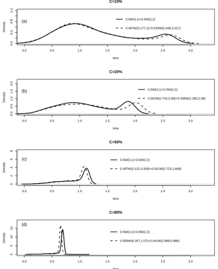
5.4 Comparison of true and estimated densities for model M1

(well-separated components) with (a) 10%, (b) 20%, (c) 50%, and (d) 80%censoring. . . 92

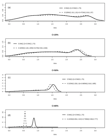
5.5 Comparison of true and estimated densities for model M2 (two

overlapping components) with (a) 10%, (b) 20%, (c) 50%, and (d) 80%censoring. . . 93

5.6 Box-plots of posterior estimates of parameters (α,β_m,π) for model

5.7 Box-plots of posterior estimates of parameters (α,β_m,π) for model M2 with five different levels of censoring. . . 95

6.1 Kaplan-Meier estimates of overall survival according to the

gene-expression subgroups. . . 123

6.2 Box-plots of the cure rates (posterior distribution ofπ) for the full DLBCL dataset, and to each of the three phenotypes (ABC, GCB

and Type III). . . 125

6.3 The posterior densities of the three models and the model averaged density for the full DLBCL dataset and each of the three

pheno-types. For comparison, the observed data is also represented as a histogram. . . 130

(21)

List of Tables

2.1 Summary of result of genes whose expression predicts survival in DLBCL. . . 14

3.1 The difference between classical and Bayesian statistical inference. . 24

4.1 Posterior summary statistics for DLBCL data . . . 68

4.2 The top five of subsets model selection for Weibull survival model . 72

4.3 Sensitivity analysis for Weibull survival model without covariates . 73

4.4 Sensitivity analysis for Weibull survival model with covariates . . . 74

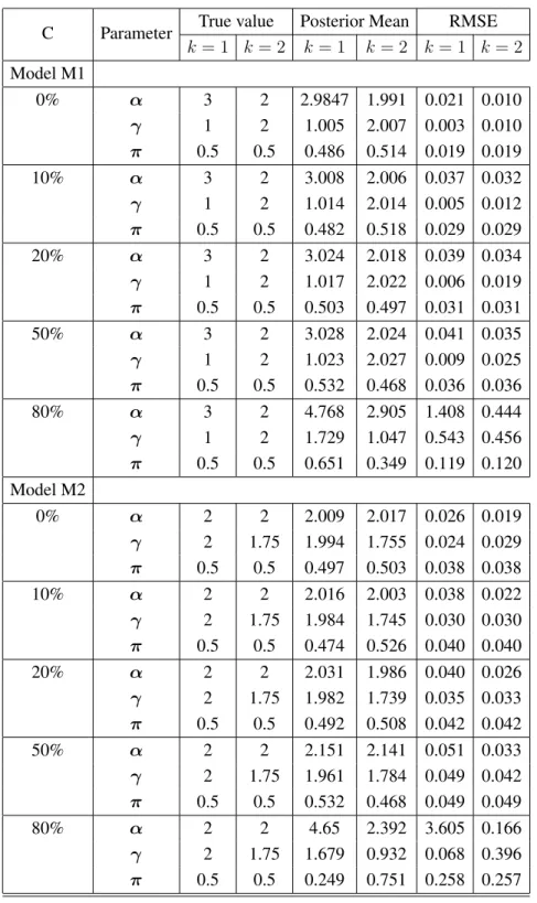
5.1 Posterior estimates of parameters (α,γ,π) and RMSE for model M1 and M2 with five different levels of censoring. . . 91

5.2 Posterior estimates of parameters (α,π,β_m) and RMSE for model M1 with five different levels of censoring. . . 96

5.3 Posterior estimates of parameters (α,π,β_m) and RMSE for model

5.4 Posterior summary statistics for DLBCL data. . . 100

5.5 Summary of posterior predictive checks for predicted survival times with five different levels of censoring. . . 101

(22)

6.1 The estimated posterior mean of the parameters, the 95%credible

intervals (CI), the BIC values and the BMA weights for each of the fitted models for the full DLBCL dataset. . . 124

6.2 The estimated posterior means of parameters, the 95% CI, BIC

values and the BMA weights for each of the models based on phe-notype for the DLBCL dataset. . . 126

6.3 The percentage of observed values that lay in the corresponding

95% credible interval for the individual models and BMA model based on the full DLBCL dataset and each of the three phenotypes. . 129

(23)

Chapter 1 Introduction

1.1 Background

In analysing the factors influencing the survival of patients with a given disease, var-ious issues can be taken into consideration as explanatory variables. Amongst these

is the biological system, in particular the gene expression of the patients. In relation to this, this research used gene expression data to aid in modelling the variability

in the patients’ survival times. These data typically come from microarrays. The significance of microarrays in genomic studies has been widely acknowledged. This

is due to the fact that microarrays can provide information about a large number of genes that may be potentially important for biological functions (Newton and

Kendziorski, 2003, Segal, 2006). This information in turn allows the examination of the variation, roles and interactions of the genes in relation to the survival time

of patients.

In this thesis, we focus on Bayesian statistical approaches to modelling survival. Although there is a large literature on Bayesian modelling and analysis, the

litera-ture on Bayesian survival is still growing and there is only limited literalitera-ture to date on Bayesian survival modelling using gene expression data and that consider model

(24)

choice issues and sensitivity analysis to censored data. For example, Kaderali et al. (2006) proposed a Bayesian Cox proportional hazards model for this purpose. In

contrast, Lee and Mallick (2004) adopted a Bayesian Weibull model, following the notion that the Weibull distribution is a popular parametric distribution for

describing survival times (Dodson, 1994).

Given the nature of microarray data to describe biological systems and outcomes of patients, and hence the potential of these covariates to produce more precise

inferences about survival, the use of a single parametric distribution to describe survival time may not be adequate. Microarray data may enable the description

of several homogeneous subgroups of patients with respect to survival time. This research therefore used Bayesian Weibull mixture models for better estimation and

prediction of this outcome. Mixture models are commonly used in describing data consisting of several groups, where each group has different properties and features

of the one family but use the same distribution. These models provide a convenient and flexible mechanism to identify and estimate distributions, which are not well

modelled by any standard parametric approaches (Stephens, 1997).

In relation to survival analysis, one fundamental issue in the use of Weibull mixture models is the effect of censored data. Censoring is an innate feature of

sur-vival and reliability data, and occurs when part of the lifetime distribution, usually at the end of the study, is unobserved. This may be due to a variety of reasons;

for example, some patients may still be alive at the end of the study period so the event of interest, namely death, has not happened. There is developing literature

on the application of Weibull mixture models in the field of survival and reliability analysis. Examples of these are Ibrahim et al. (2001b), Farcomeni and Nardi (2010),

Qian (1994) and Tsionas (2002). However, only limited attention has been paid to the effect of censoring on the mixture.

(25)

1.1. BACKGROUND 3

Models for survival analysis typically assume that everybody in the study pop-ulation is susceptible to the event of interest and will eventually experience this

event if the follow-up is sufficiently long. In recent years, there has been increasing interest in modelling survivor data with long term survivors. Most approaches to the

analysis of time to event data implicitly assume all individuals will experience the event of interest. However, there are situations when a proportion of individuals are

not expected to experience the event of interest; that is, those individuals are often referred to as immune, cured or nonsusceptible (Ibrahim et al., 2001b). To address

this issue, cure rate models are considered, which are survival models incorporating a cure fraction. These models extend the understanding of time to event data by

allowing the formulation of more accurate and informative conclusions.

The problem of model selection is abundant throughout the literature. This in-cludes both covariate selection and choice of the model itself. Some of the methods

are based on a series of significance tests (Mosler and Haferkamp, 2013) while others fit more comprehensive models; some include prior information; some use

analytic or approximate methods of estimation while others use Markov Chain Monte Carlo (MCMC) methods; different approaches use different optimisation

or model comparison criteria such us the Bayes factor (Raftery, 1996). Regardless of the method, the most common approach is to choose a single model based on

the adapted optimisation or model choice criterion. However, if a single model is selected then inferences are conditionally based on the selected model, which

often leads to excessively narrow or misleading inferences (Hjort and Claeskens, 2003, Raftery et al., 1997). This difficulty can be overcome by combining the

information provided by all suitable models into the analysis. The most common way of achieving this is to use a form of model averaging. From a Bayesian point

of view, this averaging is applied such that posterior distribution of the quantity of interest is obtained over the set of suitable models, then weighted by the respective

(26)

compare several competing models for a given dataset and to select the one “best” fits the data. Bayesian model averaging (BMA) is one way of combining models in

order to account for the uncertainty. By averaging over many different competing models, BMA incorporates model uncertainty in inference and prediction. Hence,

in this thesis, we also consider the problem of predicting survival, based on three alternatives models; a single Weibull, a mixture of Weibulls and a cure model.

In-stead of choosing a “best” model, we adopt a model averaging approach to account for model uncertainty in the prediction of survival.

1.2 Research Aims and Objectives

The primary aim of this research is to develop and apply a Bayesian modelling

approaches for prediction of patient survival using gene expression data. This research aimed to develop a new methodology that allows a better description of

genetic contributors to survival and of subgroups of patients with different survival characteristics. This can in turn provide insight into improved treatment regimes for

these patients.

Specifically, this thesis focuses on two distinct areas, covering both statistical methodology for Bayesian survival models and the application to gene expression

data. The research has the following objectives:

1. To describe and implement a Bayesian Weibull model to predict patient

sur-vival;

2. To investigate the impact of censoring on fitting a finite mixture of Weibull

distributions either with or without covariates;

3. To describe and evaluate a model averaging approach to account for model uncertainty.

(27)

1.3. STRUCTURE OF THE THESIS 5

1.3 Structure of The Thesis

This thesis is written in fulfillment of the requirement for thesis by publication. Chapters are presented here in the form which they were submitted, or accepted.

These articles are presented in Chapters 4 to 6. Each chapter has thus its own relevant literature review and there is necessarily some overlap and repetition across

chapters, and with the content of the comprehensive literature review presented in Chapters 2 and 3. Moreover, the same microarray data has been used throughout

Chapters 4 to 6 of this thesis which is repeatedly described in these chapters for the purpose of publication. Because we referred to the same papers in several chapters,

the bibliography for all chapters appears in a comprehensive bibliography at the end of the thesis.

1.4 Thesis Outline

Overall, this thesis consists of seven chapters and is outlined as follows:

Chapter 1 describes the background of the research topic and points out the research aims and objectives, and the structure of the thesis.

Chapter 2 is a literature review that related to the applied focus of this thesis,

that is, the use of gene expression in survival analysis. It covers a discussion on the basic concepts of gene expression, microarray analysis and lymphoma disease.

Chapter 3 is a literature review that provides an overview of the body of

knowl-edge associated with the research objectives and goals. The review includes a dis-cussion on survival analysis, Bayesian modelling and computation, Bayesian

vari-able selection, sensitivity analysis, goodness of fit measures and Bayesian model averaging.

(28)

Chapter 4 addresses the first issue of this study, namely describing and im-plementing Bayesian methodology to fit a Weibull distribution to predict patient

survival.

Chapter 5 addresses the second objective of this study, namely the impact of censored data on Bayesian analysis when fitting a mixture of Weibull models.

Chapter 6 is intended to meet the third objective of this research, which is to

develop a model averaging approach to incorporate the model uncertainty when predicting survival.

Chapter 7 presents the overall discussion of the research and describes how the

objectives of the thesis have been met. It highlights a summary of major findings and main contributions of this study. It also presents the implications of these

(29)

Chapter 2 Review of the role of Gene Expression in

Predicting Patient Survival

This chapter reviews literature related to the applied focus of this thesis, that is,

the use of gene expression in survival analysis. It covers a discussion on the basic concepts of gene expression, microarray analysis and lymphoma disease.

2.1 Gene Expression

The survival time of a patient suffering from a particular disease can be influenced

by various factors. One such factor is the microbiological system, specifically the gene expression of the patient.

According to the United States National Institute of Health, gene expression is

“the process by which a gene’s coded information is translated into the structures present and operating in the cell (either proteins or RNAs)” (Institute, 2013).

Sim-iliarly, Krane and Raymer (2003) define gene expression as “the process of using information that is stored in DNA to make an RNA molecule and a corresponding

protein”. Thus proteins are the main elements of cells and the production of such proteins is determined by genes, which are coded in deoxyribonucleic acid (DNA)

(30)

(Parmigiani et al., 2003).

Gene expression can therefore determine the key functions of a biological sys-tem. This is due to the fact that in genetics, gene expression constitutes the most

fundamental level at which the physical or biological features, as phenotypes, can be traced. The genetic and phenotype traits can also be influenced by environmental

factors, giving rise to gene by environment interactions. Apart from environmental aspects, the organism’s phenotype is highly associated with its related genotype.

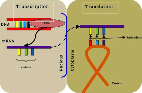
There are two main stages of protein production from genes; transcription and

translation (see Figure 2.1). Transcription involves the production of the RNA copy of a gene. One strand of DNA double helix becomes a template for RNA

polymerase to make a messenger RNA (mRNA). After maturation, this mRNA is transported to the cytoplasm from the nucleus. In translation, the protein is

produced from the mRNA template via the assembly a chain of amino acids. In this process, the ribosome binds to the mRNA at the start codon. The ribosome

continues to the elongation phase of protein synthesis. During this stage, complexes, composed of an amino acid linked to tRNA, sequentially bind to the appropriate

codon in mRNA by forming complementary base pairs with the tRNA anticodon. The ribosome moves from codon to codon along the mRNA. Amino acids are added

one by one, translated into polypeptidic sequences dictated by DNA and represented by mRNA. Finally, a release factor binds to the stop codon, terminating translation

(31)

2.2. MEASURING GENE EXPRESSION: MICROARRAY ANALYSIS 9

Figure 2.1: Gene structure and protein synthesis. Modified fromhttp://www. accessexcellence.org

2.2 Measuring gene expression: Microarray analysis

In bioinformatics, measuring gene expression plays a very central role. This

activ-ity reflects the effort to quantify the level at which a particular gene is expressed within a cell, tissue or organism. One of the common methods of measuring gene

expression, is through microarray analysis. Microarrays have been used in a range of applications such as the discovery of disease subtypes, the development of new

diagnostic tools and the identification of underlying mechanisms of disease and medicine response (Slonim and Yanai, 2009).

In order to quantify gene expression, microarray analysis typically uses a

hy-bridisation approach. The basic idea of this approach is that a glass slide or mem-brane is spotted or “arrayed” with DNA fragments or oligonucleotides that represent

(32)

specific gene coding regions. Purified RNA is then fluorescently or radioactively labeled and hybridised to the slide/membrane. In several cases, hybridisation is

carried simultaneously with reference RNA to compare data across multiple exper-iments. After thorough washing, the raw data are obtained by laser scanning or

autoradiographic imaging (World, 2013).

In the microarray analysis, there are various issues that arise. According to Slonim and Yanai (2009), these issues can be categorised into three aspects. The

first one comes from the experimental design. In this aspect, the main common issues include the selection of an appropriate array technology and the measurement

of the expression levels from each sample on a different microarray or the compar-ison of relative expression levels between a pair of samples on each microarray.

The second aspect is the preparation of microarray data for analysis, which arise issues such as the assessment of the quality of the data, is the assurance that all

samples are comparable for further analysis and the normalisation of the raw data i.e. removing the technical variation as much as possible while leaving the

biologi-cal variation untouched. The last issues of microarray analysis are from the domain of data analysis, including the use of statistical analysis software packages and the

approaches taken to analyse the microarray data in relation to the desired goal of the study. Given these issues, this research is mainly associated with the last issue as

this research utilised the microarray data that was used by Rosenwald et al. (2002) and can be downloaded athttp://llmpp.nih.gov/DLBCL/. These data, a

part from its convenient accessibility, are considered to be in accordance with the Minimum Information About a Microarray Experiment (MIAME) standard for the

(33)

2.3. THE USE OF MICROARRAYS AND GENE EXPRESSION IN THE

ANALYSIS OF LYMPHOMA 11

2.3 The use of microarrays and gene expression in the analysis

of Lymphoma

Lymphoma is a type of blood cancer that happens when the white blood cells, called lymphocytes indicate abnormal development (Pace et al., 2007, Today, 2013). This

abnormality can be shown from their uncontrollable growth or multiplication faster than normal cell or longevity longer than they should be. Lymphoma can exist

in many parts of the body and develop a dangerous mass of cell called a tumour (Hatton, 2008, Today, 2013). In Australia, lymphomas are the sixth most common

form of cancer (Australia, 2013a). Clearly, a greater understanding of lymphomas has potential to save many lives.

There are two type of the white blood cells associated with Lymphoma disease,

including the B cell and T cell lymphocytes (Australia, 2013a, Pace et al., 2007, Today, 2013). The presence of these types of cells determine the classification

of lymphoma, that is, whether it is a Hodgkin lymphoma (HL) or non-Hodgkin’s lymphoma (NHL), named after Thomas Hodgkin, who first discovered the

abnor-malities in the lymph system in 1832 (Australia, 2013a, Pace et al., 2007, Today, 2013). The HL type is related to the abnormality of the B cells, while the NHL one

is due to either the abnormal B or T cells. DBCL which is the medical context of this research is classified under the NHL (Australia, 2013a,b, Drouet, 2007, Hatton,

2008).

Diffuse large B-cell lymphoma (DLBCL) is a sub-type of NHL and the most common lymphoma worldwide (Lenza et al., 2008). DLBCL is clinically

heteroge-nous in that 35−40% of patients respond well to current therapy, the main form of which is chemotherapy, and have prolonged survival, whereas the remainder

succumb to the disease (Alizadeh et al., 2000, Lenza et al., 2008, Rosenwald et al., 2002). In general, types of this disease are very diverse both morphologically and

(34)

prognostically, and their biological properties are largely unknown, meaning that this is a relatively difficult cancer to cure and prevent (Rosenwald et al., 2002).

Traditional morphologic subclassification often results in poor reproducibility and has not been particularly helpful in predicting outcome (Hunt and Reichard, 2008).

There is some literature on relating DLBCL genotypes to phenotypes and to

survival. Alizadeh et al. (2000) identified two molecularly distinct forms of DL-BCL which had gene expression patterns indicative of different stages of B-cell

differentiation, namely genes characteristic of germinal centre B-cells (“germinal centre B-like DLBCL”) and genes normally induced during in vitro activation of

peripheral blood B cells (“activated B-like DLBCL”). They found that patients with germinal centre B-like DLBCL had significantly (p < 0.01) better overall

survival than those with activated B-like DLBCL. The molecular classification of tumours on the basis of gene expression can thus identify previously undetected and

clinically relevant subtypes of cancer (Alizadeh et al., 2000). Hunt and Reichard (2008) also reviewed gene expression profiling studies and have classified DLBCL

into two main subtypes, germinal center B-cell (GCB) and activated B-cell (ABC), with the germinal center type showing an overall better survival. They suggested

that validation of these subtypes has become possible for the practising pathologist with the use of surrogate immunohistochemical markers (Hunt and Reichard, 2008).

However, Rosenwald et al. (2002) and Rosenwald and Staudt (2003) used hierarchi-cal clustering to define subgroups of DLBCL and found that there were three

phe-notypes subgroups of patients of DLBCL; activated B-like DLBCL, germinal centre (GC)-B like and type III DLBCL. These findings support the view that the various

subgroups represent different diseases that arise as a result of distinct mechanisms of malignant transformation (Alizadeh et al., 2000, Huang et al., 2002). Based on the

hierarchical clustering, the GC B-like DLBCL had a significantly greater likelihood of survival after chemotherapy than did the activated B-like DLBCL and Type III

(35)

were differentiated from each other by distinct gene expressions of hundreds of different genes and had different survival time patterns. Similarly, Bea et al. (2005)

also identified 3 major subgroups of DLBCL: GCB, ABC, and primary mediastinal DLBCL (PMBCL).

Currently, prognostic models based on pretreatment characteristics, such as the

International Prognostic Index (IPI), are used to predict the outcome in DLBCL. IPI is the outcome predictor in DLBCL based on five clinical characteristics (age,

tumour, stage, serum lactate dehydrogenase concentration, performance status, and number of extranodal disease sites (Hatton, 2008). However, although the index is

of some value, it has not been used successfully to stratify patients for therapeutic targets (Shipp et al., 1999) (Shipp et al., 2002).

In relation to prediction of survival, Rosenwald et al. (2002) reported a

correla-tion between outcome (overall survival after chemotherapy) and gene expression data from individual microarray features, based on a Cox proportional hazards

analysis. Five genes were reportedly significant to overall survival; germinal-center B-cell (GC-B) signature, lymph-node signature, proliferation signature, BMP6 and

MHC. They concluded that DNA microarray data can be used to formulate a molec-ular predictor of survival after chemotherapy for DLBCL.

Shipp et al. (2002) reported three genes (NR4A3, PDE4B, PKC-β) that are

as-sociated with clinical outcome in the DLBCL patients by using supervised learning methods.

Lossos et al. (2004) built a predictive model for overall survival of DBLCL

patients based on six genes; LMO2, BCL6, FN1, CCND2, SCYA3 and BCL2. They used a univariate analysis to rank genes on the basis of their ability to predict

survival, then developed a multivariate model based on the expression of these six genes. Specifically, Lossos et al. (2001) showed that BCL6 has strongest prognostic

(36)

Rosenwald and Staudt (2003) used five different genes; GC-B cell signature, MHC class II, lymph node signature, proliferation signature and BMP6 to predict

DLBCL survival. They showed that gene expression is an effective tool for assess-ing the prognosis of these patients.

Lexin. (2006) proposed an integrated modelling approach, which combines

ge-nomic information, in terms of gene expression profiles, and the clinically based IPI, to predict the survival of patients with DLBCL after chemotherapy treatment.

Lexin. (2006) demonstrated that the proposed integrative modeling improved the prediction accuracy over those methods using either clinical or genomic factors

alone.

Finally, Alizadeh et al. (2011) predicted survival in DLBCL based on the ex-pression of 2 genes (LMO2, TNFRSF9) reflecting tumor and microenvironment.

They also used a multivariate Cox regression to test combinations of genes for their ability to predict survival. They concluded that the measurement of a single gene

expressed by tumor cells and a single gene expressed by the immune microenviron-ment powerfully predicts overall survival in patients with DLBCL.

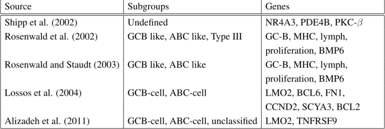
The summary of result of genes whose expression predicts survival in DLBCL

from several sources are presented in Table 2.1.

Table 2.1: Summary of result of genes whose expression predicts survival in DLBCL.

Source Subgroups Genes

Shipp et al. (2002) Undefined NR4A3, PDE4B, PKC-β

Rosenwald et al. (2002) GCB like, ABC like, Type III GC-B, MHC, lymph,

proliferation, BMP6

Rosenwald and Staudt (2003) GCB like, ABC like GC-B, MHC, lymph,

proliferation, BMP6

Lossos et al. (2004) GCB-cell, ABC-cell LMO2, BCL6, FN1,

CCND2, SCYA3, BCL2

(37)

Following the preliminary studies of gene expression in lymphoid malignancies, and particularly, DLBCL, an international consortium was established to use gene

expression profiling to provide a molecular diagnosis for all lymphoid malignancies. This consortium is known as the lymphoma/ Leukemia Molecular Profiling Project

(LLMPP). It is also hoped that it will be possible to define the molecular correlates of clinical parameters that can be used as indicators of prognosis and thus to improve

(38)

(39)

Chapter 3 Review of Statistical Methods for predicting

patient survival

This chapter provides an overview on literature related to research objectives and

goals which are reviewed within the chapters of this thesis.

3.1 Survival Analysis

3.1.1 Introduction to Survival Analysis

Survival analysis aims to estimate the three survival (survivorship, density, and

haz-ard) functions, denoted byS(t), f(t)and h(t), respectively (Collet, 1994). There exist parametric as well as non-parametric methods for this purpose (Kleinbaum and

Klein, 2005). The survival functionS(t)gives the probability of surviving beyond time t, and is the complement of the cumulative distribution function, F(t). The

hazard functionh(t)gives the instantaneous potential per unit time for the event to occur, given that the individual has survived up to time t (Kleinbaum and Klein,

2005).

3.1.2 Censored Data

In survival analysis, one must consider censored data. This is a key issue for the analysis of survival data and one of the reasons why survival analysis is a

(40)

special topic within statistics. The difference between survival analyses with other statistical analysis is the presence of censored data. In essence, censoring occurs

when there are some information about individual survival time, but the survival time is unknown exactly.

According to Miller (1998) and Hougaard (2000) data are said to be censored if

the observation time censored survival is only partial, not until the failure event. One major reason for this is that the person studied is alive when the data are evaluated,

and thus the complete lifetime is not known at that time.

There are many other reasons for censoring. For examples, the patients can be lost to follow-up, patients still alive at the end of the study or patients drop out

of the study. There are also several types of censoring, including right censoring, left censoring, interval censoring, random censoring, Type I censoring and Type II

censoring (Collet, 1994, Hosmer and Lemeshow, 1999, Kalbfleisch and Prentice, 2002, Kleinbaum and Klein, 2005). Right censoring occurs when a subject leaves

the study before an event occurs, or the study ends before the event has occurs (Kleinbaum and Klein, 2005). Left censoring occurs when the event of interest

has already occurred before enrollment (Collet, 1994). Interval censoring occurs when the survival time of each subject is only known to be within an interval (Sinha

et al., 1999). Random censoring occurs when each subject has a censoring time that is statistically independent of their failure time (Kalbfleisch and Prentice, 2002).

Type I censoring occurs when an experiment has a set number of subjects and stops at a predetermined time, at which point any subjects remaining are right censored

(Kalbfleisch and Prentice, 2002). Meanwhile, Type II censoring occurs when an experiment has a set number of subjects and stops when a predetermined number are

observed to have failed; the remaining subjects are then right censored (Kalbfleisch and Prentice, 2002).

(41)

3.1. SURVIVAL ANALYSIS 19

3.1.3 Characteristics of Survival Time Data

Survival time data have two important special characteristics (Kleinbaum and Klein, 2005) as follows:

• Survival times are non-negative, and consequently are usually positively skewed. However, we can adopt a more satisfactory approach as an alternative

distri-butional model for the original data.

• Typically, some subjects (as mentioned above) have censored survival times.

There are nonparametric and parametric approaches to modelling survival data. Some of these approaches are outlined now.

3.1.4 Kaplan-Meier

Kaplan-Meier procedure is an important and widely used tool in survival analysis

in dealing with censored data. It is a method for time to event data at each time point when a particular event takes place. The Kaplan-Meier curves have become

the standard method of displaying time to event data (Royston et al., 2008). The Kaplan-Meier method (Kaplan and Meier, 1958), also known as the product limit

estimator, which can be used to estimate the survival function from life time data. By using this method, we can make comparisons of the survival (or failure) rates

between two or more groups in order to see either the effect of particular treatments on the survival time of the patients (Royston et al., 2008) or to show the survivor

function risk groups (Kaderali et al., 2006, Rosenwald et al., 2002).

To estimate the survivor function without covariates, we can use the Kaplan-Meier estimator. This method does not rely on distributional assumptions

(dis-tribution free method). Therefore, the Kaplan-Meier estimator is categorized as a nonparametric technique (Collet, 1994, Kaplan and Meier, 1958). Given this

(42)

property, we can use the Kaplan-Meier estimator to describe many forms of the survivor function,S(t).

Let there benindividuals with observed survival timest1, . . . , tnandrbe death

times amongst the individuals, wherer ≤ n, j = 1,2, . . . , r. Ther ordered death times aret(1) < t(2) < . . . < t(r). Letnj denotes the number of individual who are

alive just before timet(j), including those who are about to die at this time, and let dj denotes the number who die at this time.

We suppose now to make the assumption that the death of the individuals in the

sample occur independently of one another. Then, the estimated survival function at any time in thekth _{constructed time interval from}_t

(k)to t(k+1),k = 1,2, . . . , r, wheret(r+1)is defined to be∞and it estimates probability of surviving beyondt(k). The Kaplan-Meier estimator of the survivor function (Collet, 1994) is given by

ˆ S(t) = k Y j=1 nj −dj nj .

The Kaplan-Meier estimator plot of the survivor function is like a step-function. The estimated survival probabilities are constant between adjacent death times and

decrease at each death time (Collet, 1994).

3.1.5 Cox Proportional Hazard

A Cox proportional hazards (PH) model is a popular mathematical model used for

modelling survival. This model was proposed by Cox and Oakes (1972) and has also come to be known as the Cox regression model. The reason why the Cox PH

model is so popular, is that because it is a semiparametric and a “robust” model. The results from using this model will closely approximate the results of the correct

parametric model (Kleinbaum and Klein, 2005).

A survival analysis typically examines the relationship of the survival distri-bution to covariates. If the risk of failure at a given time depends on the value

(43)

3.1. SURVIVAL ANALYSIS 21

of x1, x2, . . . , xp of p predictor variables X1, X2, . . . , Xp, then the value of these

variables are assumed to have the time origin. If h0(t) is the hazard function for each object with the value of all predictor variableX is zero, then the function of h0(t)are the baseline hazard function (Collet, 1994). The Cox PH model is usually written in terms of the hazard model as follows

h(t) =h0(t) exp(β1X1 +β2X2+. . .+βpXp). (3.1)

There are two basic assumptions of this model; the effect of X is linear andβ

is constant over time. The latter being the assumption of a proportional hazards. It is also assumed that individuals are independent and homogeneous given their

covariates (Andersen, 1991).

An important feature of equation 3.1, which concerns the PH assumption, is that the baseline hazard is a function oft, but does not involve theX’s (Kleinbaum and

Klein, 2005). In contrast, the exponential expression shown here, involves theX’s, but does not involve t. Then, X’s here are called time independent X’s. Another

important property of the Cox model is that the baseline hazard, h0(t), can be an unspecified function. This property that makes the Cox PH model a semiparametric

model (Hosmer and Lemeshow, 1999, Kleinbaum and Klein, 2005). In contrast, a parametric model is one whose functional form is completely specified, except for

the values of the unknown parameters. For example, the Weibull PH model.

3.1.6 Frailty Model

The Cox proportional hazards (PH) model can be extended to allow time dependent variables as predictors (Kleinbaum and Klein, 2005). Frailty models are extensions

of the PH model which is an known as the Cox model (Cox and Oakes, 1972). The aim of this model is to account for unobserved heterogeneity that is caused by

(44)

unmeasured covariates (Hougaard, 1995). In statistical terms, a frailty model is a random effect model for time to event data, where the random effect (the frailty)

has a multiplicative effect on the baseline hazard function (Duchateau and Janssen, 2008). Conditional on the frailty, the survival times are assumed to be independent

with PH structure. The modeling process is then completed by assuming multilevel frailty effects (Kima and Dey, 2008).

3.1.7 Parametric Survival Model

A parametric survival model is one in which survival time (the outcome) is as-sumed to follow a known distribution (Hosmer and Lemeshow, 1999, Kleinbaum

and Klein, 2005). The distributions that are commonly used for survival time are; the Weibull (Collet, 1994, Ibrahim et al., 2001b), the exponential (a special case

of the Weibull) (Collet, 1994, Ibrahim et al., 2001b, Sparling et al., 2006), the log-logistic, the log-normal, and the generalized gamma (Ibrahim et al., 2001b).

Survival estimates were obtained from parametric survival models typically

yield plots more consistent with a theoretical survival curve. If the investigator is comfortable with the underlying distributional assumption, then the parameters

can be estimated and the survival and hazard functions can be specified as well (Kleinbaum and Klein, 2005). This simplicity and completeness of a parametric

approach makes statistical tests more powerful.

For parametric survival models, time to event is assumed to follow certain dis-tribution whose probability density function (pdf)f(t)can be expressed in terms of

unknown parameters (Collet, 1994). Once a probability density function is specified for survival time, the corresponding survival and hazard functions can be

deter-mined.

Survival methods using the Bayesian statistical framework have been collated more recently in the well regarded texts of Gelman et al. (2004), Ibrahim et al.

(45)

3.2. BAYESIAN MODELLING 23

(2001b) and Congdon (2006), with expanded applications in Congdon (2003).

3.2 Bayesian Modelling

3.2.1 Overview of Bayesian Approach

Modern Bayesian analysis began with a posthumous publication in 1763 by

Rev-erend Thomas Bayes that set the theoretical framework and after a status of around 200 years, publications by Geman and Geman (1984) and Bernando and Smith

(1994), among others, exploited computer technology and computational algorithms, and extended the modelling framework.

The idea of Bayesian statistics within the context of life data analysis is to

integrate prior knowledge, along with a given set of current observations, in order to make statistical inferences. The prior information could come from operational

or observational data, from previous comparable experiments or from engineering knowledge (Gelman et al., 2004). This type of analysis can be mainly useful when

there is limited test data for a given design. By integrating prior information about the parameters, a posterior distribution for the parameters can be obtained and

inferences on the model parameters and their functions can be made.

Supposeθis some quantity that is unknown and letp(θ)denote the prior distri-bution ofθ. Next, letybe some observed data, whose probability of occurrence is

assumed to depend onθ. This dependence is formalized byp(y |θ), the conditional probability ofyfor each possible value ofθ, and when considered as a function ofθ

is known as the likelihood (Spiegelhalter et al., 2004). The probability for different values ofθ, taking account ofyis denoted byp(θ |y).

Bayes’ theorem applied to a general quantity says that:

p(θ |y) = p(y|θ)p(θ)

p(y) .

(46)

R

p(θ |y)dθ = 1, so that

p(θ|y)∝p(y|θ)p(θ),

which says that the posterior distribution is proportional to the product of the likeli-hood and the prior (Gelman et al., 2004, p.7-9).

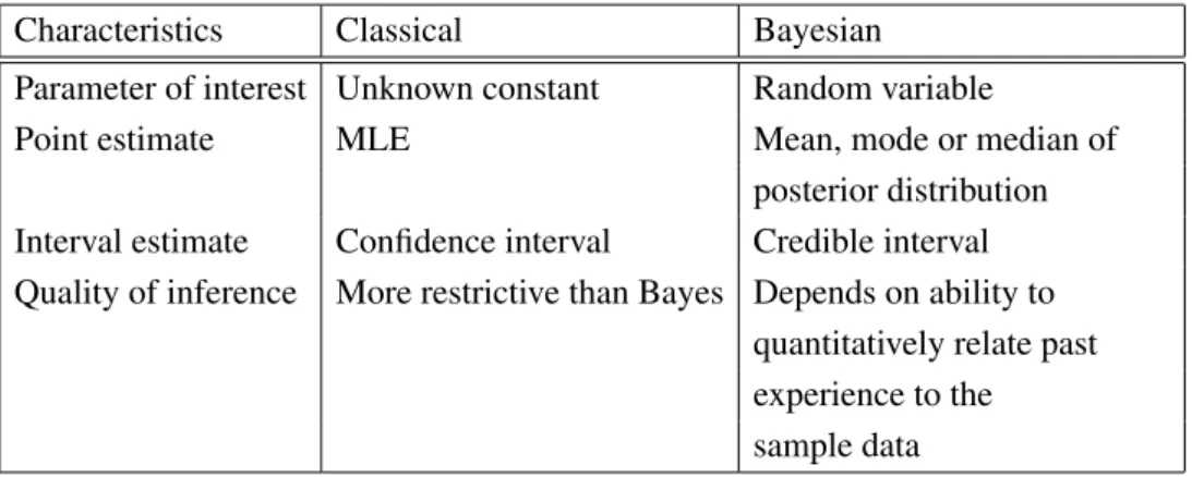
The main differences between classical statistical inference and Bayesian

statis-tical inference is shown in Table 3.1 (Gelman, 2008).

Table 3.1: The difference between classical and Bayesian statistical inference.

Characteristics Classical Bayesian

Parameter of interest Unknown constant Random variable

Point estimate MLE Mean, mode or median of

posterior distribution

Interval estimate Confidence interval Credible interval

Quality of inference More restrictive than Bayes Depends on ability to

quantitatively relate past experience to the sample data

3.3 Prior Distribution

Prior distributions play a very important role in Bayesian statistics. There are

two different types of prior distributions; informative and non-informative (Gelman et al., 2004, Marin and Robert, 2007, Spiegelhalter et al., 2004). Non-informative

prior distributions (vague, flat, and diffuse) play a minimal role in posterior in-ference, and posterior can be sensitive to prior (Gelman et al., 2004). The

non-informative prior distributions can be used to make inferences that are not greatly affected by external information or when external information is not available

(Gel-man et al., 2004, Marin and Robert, 2007, Spiegelhalter et al., 2004).

Informative priors have a stronger influence on the posterior distribution. The influence of the prior distribution on the posterior is related to the relative variance

(47)

3.4. BAYESIAN COMPUTATION 25

of the data and the prior. We can obtained informative priors from past data or expert information (Gelman et al., 2004, Marin and Robert, 2007, Spiegelhalter

et al., 2004).

Other categorisations of prior include conjugate prior, proper prior and improper prior (Jeffreys prior) (Gelman et al., 2004, Marin and Robert, 2007, Spiegelhalter

et al., 2004). Several papers have been published on Bayesian survival analysis that consider some very general constructions and applications of reference priors, other

than the normal prior. Among these are critical issues in Ibrahim and Laud (1991), who examine Jeffreys’s prior for class of generalized linear models and Kim and

Ibrahim (2000) who discusses non-informative priors for linear combinations of the means under the normal population. Other scholars, Berger and Bernardo (1989),

have examined reference priors for estimating a product of means. Bernardo (1997), specifically, examines the existence of non-informative priors.

Bayesian methods provide a practical and effective tool for microarray analysis

(Baldi and Long, 2001, Gottardo, 2003, Ibrahim et al., 2002, Lewin et al., 2005). The DNA microarray technology has important applications in gene expression data

analysis. However, the potential sources of random and systematic measurement er-rors are a critical issue in statistical analysis. It is impossible to propose a statistical

model that reflects all sources of errors. Therefore, a good model should capture the most essential features of the data.

3.4 Bayesian Computation

Bayesian computation generally exploits modern computer power to carry out

simu-lations (Spiegelhalter et al., 2004) based on Markov chains and is known as Markov chain Monte Carlo (MCMC). Monte Carlo methods are techniques that have the aim

of evaluating integrals rather than exact or approximate algebraic analysis (Spiegel-halter et al., 2004). Several MCMC algorithms that are commonly used are Gibbs

(48)

sampling, Metropolis-Hastings, reversible jump, slice sampling, particle filters, per-fect sampling and adaptive rejection sampling (Marin and Robert, 2007,

Spiegelhal-ter et al., 2004).

Three MCMC algorithms will be used in this research, namely Gibbs sampling, Metropolis-Hastings and slice sampling. Gibbs sampling is an algorithm to generate

a sequence of samples from the joint probability distribution of two or more random variables, with the purpose of approximating the joint distribution. Gibbs sampling

is applicable when the joint distribution is not known explicitly, but the conditional distribution of each variable is known (Gelman et al., 2004). Moreover, the Gibbs

sampling algorithm is a method to generate an instance from the distribution of each variable in turn, conditional on the current values of the other variables (Gelman

et al., 2004). Meanwhile, the Metropolis-Hastings algorithm is a rejection sampling algorithm used to generate a sequence of samples from a probability distribution

that is difficult to sample from directly. This sequence can be used in MCMC simulation to approximate the distribution, or to compute an integral (such as an

expected value) (Hastings, 1970). The Gibbs sampling algorithm is a special case of the Metropolis-Hastings algorithm which is usually faster and easier to use but is

less generally applicable (Chib and Greenberg, 1995).

Furthermore, Neal (2003) described a class of “slice sampling” methods that can be applied to sample from a wide variety of distributions. “slice sampling” is a type

of MCMC algorithm for drawing random samples from a statistical distribution. The method is based on the observation that to sample a random variable one can

sample uniformly from the region under the graph of its density function (Damien et al., 1999, Mira and Tierney, 2002, Neal, 2003, Tibbits et al., 2011). Simple forms

of univariate slice sampling are an alternative to Gibbs sampling that avoids the need to sample from nonstandard distributions (Neal, 2003).

(49)

hand-tailored sampling programs. However, the WinBUGS software is widely used in a variety of applications (Marin and Robert, 2007).

3.4.1 Weibull and Mixture Survival Models Weibull Model

The Weibull model is perhaps the most widely used parametric survival model in reliability (Kim and Ibrahim, 2000, Murthy et al., 2004) to characterize the

probabilistic behaviour of a large number of real world phenomena (Kaminskiy and Krivtsov, 2005). A detailed review of the Weibull model can be found in Murthy

et al. (2004). Because of its various shapes of the probability density function (pdf) and its convenient representation of the distribution/ survival function, the Weibull

distribution has been used very effectively for analyzing lifetime data, particularly when the data are censored, which is very common in most life testing experiments

(Collet, 1994, Kundu, 2008).

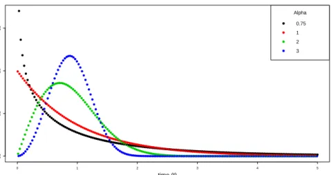
Suppose we have independent identically distributed (i.i.d) survival times t = (t1, t2, . . . , tn)0, which follow a Weibull distribution, denoted by W(α, γ) with a

shape parameterαand a scale parameterγ. The parameterαrepresents the failure rate behavior. Ifα < 1, the failure rate decreases with time; if α > 1, the failure

rate increases with time; whenα = 1, the failure rate is constant over time, which indicates an exponential distribution. The parameterγ has the same units ast, such

as years, hours, etc. A change inγhas the same effect on the distribution as a change of the abscissa scale. Increasing the value ofγ while holding α = 1constant has

the effect of stretching out the pdf. Ifγ is increased, the distribution is stretched to the right and its height decreases, while maintaining its shape. Ifγis decreased, the

distribution is pushed in towards the left and its height increases (Figures 3.1 and 3.2) (Rinne, 2008, p.27-43).

(50)

0 1 2 3 4 5 1 2 3 4 5 time(t) failure time (h(t)) alpha=1.5, gamma=1 alpha=1, gamma=1 alpha=0.5, gamma=1

Figure 3.1: Weibull failure distribution with differing parameter values.

● ● ● ● ● ● ● ● ● ● ● ● ● ● ● ● ● ● ● ● ● ● ● ● ● ● ● ●● ● ● ●● ● ● ● ● ● ● ● ● ● ● ● ● ● ● ● ● ● ● ● ● ● ● ● ●● ● ● ● ● ● ● ● ● ● ● ● ● ● ● ● ● ● ● ● ● ● ● ● ● ● ● ● ● ● ● ● ● ● ● ● ● ● ● ● ● ● ● ● ● ● ● ● ● ● ● ● ● ● ● ● ● ● ● ● ● ● ● ● ● ● ● ● ● ● ● ● ● ● ● ● ● ● ● ● ● ● ● ● ● ● ● ● ● ● ● ● ● ● ● ● ● ● ● ● ● ● ● ● ● ● ● ● ● ● ● ● ● ● ● ● ● ● ● ● ● ● ● ● ● ● ● ● ● ● ● ● ● ● ● ● ●● ● ● ● ● ● ● ● ● ● ● ● ● ● ● ● ● ● ● ● ● ● ● ● ● ● ● ● ●● ● ● ● ● ●● ● ● ●● ● ●● ● ● ● ●● ● ●●● ● ● ●● ● ●●● ● ● ● ● ● ●● ● ● ● ● ● ● ●● ● ● ● ● ● ● ●● ● ● ● ● ● ● ●● ● ● ● ● ● ● ●● ● ● ● ● ● ● ●● ● ● ● ● ● ● ●● ● ● ● ● ● ● ●● ● ● ● ● ● ● ●● ● ● ● ● ● ● ●● ●● ● ● ● ● ●● ●● ● ● ● ● ●● ●● ●● ● ● ●● ●● ●● ● ● ●● ●● ●● ● ● ●● ●● ●● ● ● ●● ●● ●● ● ● ●● ●● ●● ● ● ● ● ●● ●● ● ● ● ● ●● ●● ● ● ● ● ●● ●● ● ● ● ● ●● ●● ● ● ● ● ●● ●● ●● ● ● ●● ●● ●● ● ● ●● ●● ●● ● ● ●● ●● ●● ● ● ●● ●● ●● ● ● ● ● ●● ●● ● ● ● ● ●● ●● ● ● ● ● ●● ●● ● ● ● ● ●● ●● ● ● ● ● ●● ●● ● ● ● ● ●● ●● ●● ● ● ●● ●● ●● ● ● ●● ●● ●● ● ● ●● ●● ●● ● ● ●● ●●●●●●●●●●●●●●●●●●●●●●●●●●●●●●●●●●●●●●●●●●●●●●●●●●●●●●●●●●●●●●●●●●●●●●●●●●●●●●●●●●●●●●●●●●●●●●●●●●●●●●●●●●●●●●●●●●●●●●●●●●●●●●●●●●●●●●●●●●●●●●●●●●●●●●●●●●● 0 1 2 3 4 5 0.0 0.5 1.0 1.5 time (t) f(t) ● ● ● ● Alpha 0.75 1 2 3

Figure 3.2: Weibull densities with different values of the shape parameter.

The density function for Weibull distributed survival times is as follows:

f(ti |α, γ) =      αγtα_i−1exp(−γtα i), ti >0, α >0, γ >0 0, otherwise.

(51)

Since the logarithm of the Weibull hazard is a linear function of the logarithm of time, it is more convenient to write the model in terms of the parameterization

λ= log(γ)(Ibrahim et al., 2001b), so that:

f(ti |α, λ) =αtiα−1exp(λ−exp(λ)t α

i)

The corresponding survival function and the hazard function, using the λ pa-rameterization, are as follows:

S(ti |α, λ) = exp(−exp(λ)tαi),

h(ti |α, λ) = f(ti |α, λ)/S(ti |α, λ) =αexp(λ)tαi−1.

The likelihood function of(α, λ)is as follows:

L(α, λ|D) = n Y i=1 f(ti |α, λ)δiS(ti |α, λ)(1−δi) = αdexp{dλ+ n X i=1 (δi(α−1) log(ti)−exp(λ)tαi)}, whereD= (t, δ),d=Pn i δiandδi as follows δi =     

1, if the lifetime is uncensored, i.e.,Ti =ti.

0, if the lifetime is censored, i.e.,Ti > ti.

Let xij be the jth covariate associated with ti for j = 1,2, . . . , p + 1. The

covariate data can be included into the model through λ. Given that λ must be positive, one option is to include the covariates as follows:

γi = exp(x0iβ),so that

(52)

whereβ= (β1, β2, . . . , βp)is the vector of regression parameter.

Thus, the log-likelihood function becomes:

logL(α,β|D) = n X i=1 δi log(α) + (α−1) log(ti) +x0_iβ −exp(x0_iβ)tα_i.

We can also extend equation (3.2) to include additional variation, i, perhaps

due to explanatory variables that are not included in the model. In this case, we

obtain:

λi =x0iβ+i, (3.3)

wherei ∼N(0, σ2).

Bayesian Weibull Model

Prior information might include one or more of the model parameters. The

integra-tion of such prior informaintegra-tion into model (3.1) could be expressed in the form of a probability density,p(θ, β|H), whereH represents the background information. This prior density is then combined with the observed data, in the form of the like-lihood, using Bayes’ Theorem. Thus, the posterior joint density,p(θ, β|H, data), is proportional to the product of the likelihood and the prior density,p(θ, β|H).

In a microarray setting, one of the regression parameters may represent a gene expression, about which there will be prior information available (Kaderali et al.,

2006, Tachmazidou et al., 2008). This may take either the expert belief or the results from the analysis of similar studies.

In a complex model, the posterior densities can often be too difficult to work

with directly (Bolstad, 2010, Ibrahim et al., 2001b, Omurlu et al., 2009). To update knowledge about the parameters requires that one can sample from the posterior

(53)

density. With MCMC methods, it is possible to generate samples from a posterior density and to use these samples to approximate expectations of quantities of

in-terest. MCMC method samples successively from a target distribution, with each sample drawn depending on the previous one (see Section 3.4).

Some papers have appeared on the Bayesian approach to Weibull survival

mod-elling. Among these are Abrams et al. (1996) who analyzed parametric propor-tional hazards models in clinical data. Kostoulas et al. (2010) examined a Bayesian

Weibull survival model for time to infection data measured with delay, and Kundu (2008) also analysed the Bayesian inference of unknown parameters of the

progres-sively censored Weibull distribution. Other scholars, Ahmed et al. (2010) analysed the comparison of the Bayesian and maximum likelihood estimation for Weibull

distribution and Kaminskiy and Krivtsov (2005) proposed a simple procedure for Bayesian estimation of the Weibull distribution. However, the literature on Bayesian

survival is still growing and there is limited literature to date on Bayesian survival modelling using gene expression and consider model choice issues and sensitivity

analysis, e.g. Weibull model.

Under the assumptions stated in Section 3.4.1, a Bayesian formulation of the Weibull model takes the form

ti ∼W(ti |α, λ), i= 1,2, ..., n.

α∼p(α|θα).

λ∼p(λ|θλ),

where θα andθλ are the hyperparameters of the prior distribution of α and λ,

re-spectively. In this model, inference may initially focus on the posterior distribution of the shape parametersαand the scale parameterλ.

(54)

posterior distribution of(α, λ)is given by

p(α, λ|D)∝L(α, λ|D)p(α)p(λ).

Since the joint posterior distribution of(α, λ |D)does not have a closed form, we use MCMC methods for computation (Gilks et al., 1996). Given the conditional distributions defined in Algorithm 1, the conditional distribution ofλdoes not have

an explicit form.

Algorithm 1Weibull survival model without covariates 1: k = 0, Set initial values[α0_{, λ}0_]

Fork = 1 :K, whereKis large,

2: Sampleα(t+0) ∼α|λ(t), D, fori= 1,2, ..., n 3: Sampleλ(t+0) _∼_λ_|_α(t)_{, D, for}_i_{= 1}_,₂_{, ..., n} 4: Setk =k+ 1and go to step 1

5: Continue required number of iterations 6: Stop

In order to build a Weibull model with covariates, we develop a hierarchical model, introducing the covariatesxi throughλusing the equation (3.3).

The joint posterior distribution of(α,β)is given by

p(β, α |D)∝L(α,β |D)p(α)p(β)

MCMC analysis is done using the conditional distributions of the parameters, as described in Algorithm 2. As discussed earlier, the conditional distribution of αdoes not have an explicit form and as such can be sampled from approximately

(55)

Algorithm 2Weibull survival model with covariates 1: k= 0, Set initial values[α0_{, β}0_]

Fork= 1 : K, whereK is large,

2: Sampleα(t+0) _∼_α _|_β(t)_{, D, for}_i_{= 1}_,₂_{, ..., n} 3: Sampleβ(t+0) _∼_λ_|_α(t)_{, D, for}_i_{= 1}_,₂_{, ..., n} 4: Setk =k+ 1and go to step 1

5: Continue required number of iterations 6: Stop

3.4.2 Mixture Weibull Models

In many cases, the application of a single parametric distribution is not sufficient to

describe the complexity of the data being observed. For instance, the data may have been generated from several (possibly uncensored) homogenous subgroups. To

produce an appropriate inference, these groups should be taken into consideration.

Mixture models are usually used in modelling data consisting of several groups, where each group has different properties and characteristics of the one family but

use the same distribution. This model provides a convenient and flexible mechanism for identification and estimation of distributions which are not well modelled by

any standard parametric family (Stephens, 1997). This is achieved by assuming that the observed data can be represented by a weighted sum of distributions, with

each distribution defined by a unique parameter set representing a subspace of the population.

Weibull mixture models have received increasing attention in recent statistical

research with applications in the field of survival and reliability analysis. The advances in EM algorithm (Dempster et al., 1977), the Bayesian paradigm (Berger,

1985), (Besag et al., 1995), and MCMC computational methods (Diebolt and Robert, 1994) have substantially expanded the methodology and application of Weibull

mix-ture models. For example, in the Bayesian context, Marin et al. (2005a) described methods to fit a Weibull mixture model with an unknown number of components.

(56)

Chen et al. (1985) used a two component mixture model for the analysis of cancer survival data, generalizing an earlier idea by Berkson and Gage (1952). Similarly,

Farcomeni and Nardi (2010) proposed a two component mixture to describe survival times after an invasive treatment. Qian (1994) also used a mixture of a Weibull

component and a surviving fraction in the context of a lung cancer clinical trial. Tsionas (2002) considered a finite mixture of Weibull distributions with a larger

number of components for capturing the form of a particular survival function.

There is developing literature for fitting mixture models to censored data. For example, Miyata (2011) used the maximum likelihood estimator for fitting a

mix-ture of exponential distributions and a mixmix-ture of normal distributions with censored data, and Hanson (2006) modelled censored lifetime data using a mixture of

gam-mas. An overview can be found in Ibrahim et al. (2001b). However, there is limited attention to Bayesian mixture models in the field of survival analysis, e.g. Weibull

mixture and limited attention to the effect of censoring on the mixture.

Initially, we assume that we observe survival timeton patients possibly from a heterogeneous population. As in Section 3.4.1, the two parameter Weibull density

function for survival time is given by

W(t |α, γ) =αγtα−1exp (−γtα),

for α > 0 and γ > 0, where α is a shape parameter and γ is a scale parameter

(Ibrahim et al., 2001b). A mixture of K Weibull densities is defined by (Marin et al., 2005a) f(t|K,π,α,γ) = K X m=1 πmW(t|αm, γm), (3.4)

whereα = (α1, . . . , αK), γ = (γ1, . . . , γK), are the parameters of each Weibull

distribution andπ = (π1, . . . , πK) is a vector of nonnegative weights that sum to

(57)

Let xij be the jth covariate associated with patient i, for j = 1,2, . . . , p. The

covariates can be included in the model as follows (Farcomeni and Nardi, 2010)

log(γm) =x0iβm =λm, (3.5)

where xi = (xi1, . . . , xip), γm = (γ1m, . . . , γpm) and βm = (β1m, . . . , βpm), for

i= 1,2, . . . , nandm= 1,2, . . . , K.

We now assume that we observe possibly right censored data for n patients;

y = (y1, . . . , yn) whereyi = (ti, δi) andδi is an indicator function (Marin et al.,

2005a) such that

δi =     

1, if the lifetime is uncensored, i.e.,Ti =ti.

0, if the lifetime is censored, i.e.,Ti > ti.

Thus, the likelihood function becomes

L(π,α,γ |K, ti, δi,x)∝ n Y i=1 f(ti |K,π,α,γ,x) δi S(ti |K,π,α,γ,x) 1−δi . Here, the incomplete information is modelled via the survivor function, which

reflects the probability that the patient was alive for duration greater thanti.

Bayesian Mixture Weibull Models

In WinBUGS (Lunn et al., 2000, Ntzoufras, 2009, Spiegelhalter et al., 2002), pos-sibly right censored data can be modelled using a missing data approach via the