CONVOLVED GAUSSIAN PROCESS
PRIORS FOR MULTIVARIATE
REGRESSION WITH APPLICATIONS
TO DYNAMICAL SYSTEMS
A thesis submitted to the University of Manchester for the degree of Doctor of Philosophy
in the Faculty of Engineering and Physical Sciences
2011
Mauricio A. ´Alvarez
List of Figures 5 List of Tables 9 Abstract 11 Declaration 12 Copyright 13 Acknowledgements 14 Notation 15 1 Introduction 17
2 Covariance functions for multivariate regression 24
2.1 Kernels for multiple outputs . . . 25
2.1.1 The linear model of coregionalization . . . 26
2.1.2 Process convolutions for multiple outputs . . . 34
2.2 Multivariate Gaussian Process Priors . . . 44
2.2.1 Parameter estimation . . . 45
2.2.2 Prediction . . . 47
2.3 Multivariate regression for gene expression . . . 50
2.4 Summary . . . 55
3 Linear Latent force models 56 3.1 From latent variables to latent forces . . . 57
3.2 From latent forces to convolved covariances . . . 59
3.2.2 Higher-order Latent Force Models . . . 63
3.2.3 Multidimensional inputs . . . 65
3.3 A Latent Force Model for Motion Capture Data . . . 65
3.4 Related work . . . 68
3.5 Summary . . . 73
4 Efficient Approximations 75 4.1 Latent functions as conditional means . . . 77
4.1.1 Posterior and predictive distributions . . . 83
4.1.2 Model selection in approximated models . . . 86
4.2 Regression over gene expression data . . . 86
4.3 Variational approximations . . . 90
4.3.1 A variational lower bound . . . 91
4.3.2 Variational inducing kernels . . . 93
4.4 Related work . . . 97
4.5 Summary . . . 100
5 Switching dynamical latent force models 101 5.1 Second order latent force models . . . 103
5.2 Switching dynamical latent force models . . . 105
5.2.1 Definition of the model . . . 105
5.2.2 The covariance function . . . 109
5.3 Segmentation of human movement data . . . 111
5.4 Related work . . . 113
5.5 Summary . . . 114
6 Conclusions and Future Work 115
Reprint of publication I 119
Reprint of publication II 120
Reprint of publication III 121
Reprint of publication IV 122
List of Figures
1.1 Examples of the type of problems that we consider in this thesis. . 18 1.2 An example of a walking exercise. In 1.2(a), there are missing
poses that are filled in 1.2(b). . . 18 2.1 Predictive mean and variance for genes FBgn0038617 (first row)
and FBgn0032216 (second row) using the linear model of coregion-alization (figures 2.1(a) and 2.1(c)) and the convolved multiple-output covariance (figures 2.1(b) and 2.1(d)) with Q = 1 and Rq = 1. The training data comes from replicate 1 and the testing data from replicate 2. The solid line corresponds to the predictive mean, the shaded region corresponds to 2 standard deviations of the prediction. Performances in terms of SMSE and MSLL are given in the title of each figure and appear also in table 2.2. The adjectives “short” and “long” given to the length-scales in the cap-tions of each figure, must be understood relative to each other. . . 52 2.2 Predictive mean and variance for genes FBgn0010531 (first row)
and FBgn0004907 (second row) using the linear model of coregion-alization (figures 2.2(a) and 2.2(c)) and the convolved multiple-output covariance (figures 2.2(b) and 2.2(d)) with Q = 1 and Rq = 1. The difference with figure 2.1 is that now the training data comes from replicate 2 while the testing data comes from replicate 1. The solid line corresponds to the predictive mean, the shaded region corresponds to 2 standard deviations of the predic-tion. Performances in terms of SMSE and MSLL are given in the title of each figure. . . 54
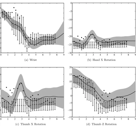
and from direct regression from the humerus angles (crosses with stick error bars). For these examples noise is high due to the relatively small length of the bones. Despite this the latent force model does a credible job of capturing the angle, whereas direct regression with independent GPs fails to capture the trends. . . . 69
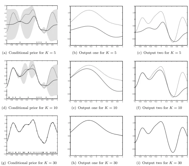
4.1 Conditional prior and two outputs for different values of K. The first column, figures 4.1(a), 4.1(d) and 4.1(g), shows the mean and confidence intervals of the conditional prior distribution using one input function and two output functions. The dashed line represents a sample from the prior. Conditioning over a few points of this sample, shown as black dots, the conditional mean and conditional covariance are computed. The solid line represents the conditional mean and the shaded region corresponds to 2 standard deviations away from the mean. The second column, 4.1(b), 4.1(e) and 4.1(h), shows the solution to equation (2.11) for output one using a sample from the prior (dashed line) and the conditional mean (solid line), for different values of K. The third column, 4.1(c), 4.1(f) and 4.1(i), shows the solution to equation (2.11) for output two, again for different values of K. . . 78
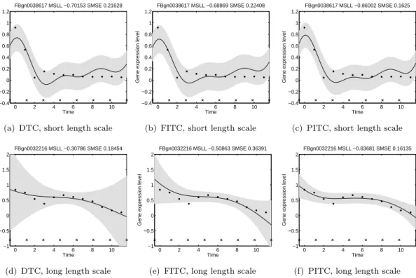
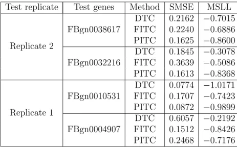
4.2 Predictive mean and variance for genes FBgn0038617 (first row) and FBgn0032216 (second row) using the different approximations. In the first column DTC (figures 4.2(a) and 4.2(d)), second column FITC (figures 4.2(b) and 4.2(e)) and in the third column PITC (fig-ures 4.2(c) and 4.2(f)). The training data comes from replicate 1 and the testing data from replicate 2. The solid line corresponds to the predictive mean, the shaded region corresponds to 2 stan-dard deviations of the prediction. Performances in terms of SMSE and MSLL are given in the title of each figure. The crosses in the bottom of each figure indicate the positions of the inducing points. 88
4.3 Predictive mean and variance for genes FBgn0010531 (first row) and FBgn0004907 (second row) using the different approximations. In the first column DTC (figures 4.3(a) and 4.3(d)), second column FITC (figures 4.3(b) and 4.3(e)) and in the third column PITC (figures 4.3(c) and 4.3(f)). The training data comes now from replicate 2 and the testing data from replicate 1. The solid line corresponds to the predictive mean, the shaded region corresponds to 2 standard deviations of the prediction. Performances in terms of SMSE and MSLL are given in the title of each figure. The crosses in the bottom of each figure indicate the positions of the inducing points, which remain fixed during the training procedure. 89 4.4 With a smooth latent function as in (a), we can use some
induc-ing variables uq (red dots) from the complete latent process uq(x) (in black) to generate smoothed versions (for example the one in blue), with uncertainty described by p(uq|uq). However, with a white noise latent function as in (b), choosing inducing variables uq (red dots) from the latent process (in black) does not give us any information about other points (for example the blue dots). In (c) the inducing functionλq(x) acts as a surrogate for a smooth function. Indirectly, it contains information about the inducing points and it can be used in the computation of the lower bound. In this context, the symbol ∗refers to the convolution integral. . 95 5.1 Representation of an output constructed through a switching
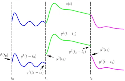
dy-namical latent force model with Q = 3. The initial conditions yq(t
q−1) for each interval are matched to the value of the output in the last interval, evaluated at the switching point tq−1, this is, yq(t
q−1) = yq−1(tq−1−tq−2). . . 108 5.2 Joint samples of a switching dynamical LFM model with one
out-put, D = 1, and three intervals, Q= 3, for two different systems. Dashed lines indicate the presence of switching points. While sys-tem 2 responds instantaneously to the input force, syssys-tem 1 delays its reaction due to larger inertia. . . 108 5.3 Data collection was performed using a Barrett WAM robot as
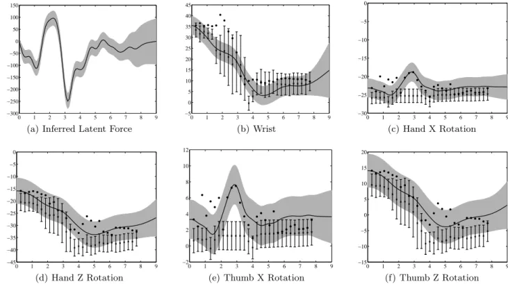
movement data collected as in figure 5.3 leads to plausible segmen-tations of the demonstrated trajectories. The first row corresponds to the lower bound, latent force and one of four outputs, humeral rotation (HR), for trial one. Second row shows the same quanti-ties for trial two. In this case, the output corresponds to shoulder flexion and extension (SFE). Crosses in the bottom of the figure refer to the number of points used for the approximation of the Gaussian process, in this caseK = 50. . . 112
List of Tables
2.1 Standardized mean square error (SMSE) and mean standardized log loss (MSLL) for the gene expression data for 50 outputs. CMOC stands for convolved multiple output covariance. The experiment was repeated ten times with a different set of 50 genes each time. Table includes the value of one standard deviation over the ten repetitions. More negative values of MSLL indicate better models. 51 2.2 Standardized mean square error (SMSE) and mean standardized
log loss (MSLL) for the genes in figures 2.1 and 2.2 for LMC and CMOC. Gene FBgn0038617 and gene FBgn0010531 have a shorter length-scale when compared to the length-scales of genes FBgn0032216 and FBgn0004907. . . 53 3.1 Root mean squared (RMS) angle error for prediction of the left
arm’s configuration in the motion capture data. Prediction with the latent force model outperforms the prediction with regression for all apart from the radius’s angle. . . 68 4.1 Standardized mean square error (SMSE) and mean standardized
log loss (MSLL) for the gene expression data for 1000 outputs using the efficient approximations for the convolved multiple output GP. The experiment was repeated ten times with a different set of 1000 genes each time. Table includes the value of one standard deviation over the ten repetitions. . . 87 4.2 Standardized mean square error (SMSE) and mean standardized
log loss (MSLL) for the genes in figures 4.2 and 4.3 for DTC, FITC and PITC withK = 8. . . 89
1000 outputs using the efficient approximations for the convolved multiple output GP. The experiment was repeated ten times with a different set of 1000 genes each time. . . 90
Abstract
In this thesis we address the problem of modeling correlated outputs using Gaus-sian process priors. Applications of modeling correlated outputs include the joint prediction of pollutant metals in geostatistics and multitask learning in machine learning. Defining a Gaussian process prior for correlated outputs translates into specifying a suitable covariance function that captures dependencies between the different output variables. Classical models for obtaining such a covariance func-tion include the linear model of coregionalizafunc-tion and process convolufunc-tions. We propose a general framework for developing multiple output covariance functions by performing convolutions between smoothing kernels particular to each output and covariance functions that are common to all outputs. Both the linear model of coregionalization and the process convolutions turn out to be special cases of this framework. Practical aspects of the proposed methodology are studied in this thesis. They involve the use of domain-specific knowledge for defining relevant smoothing kernels, efficient approximations for reducing computational complexity and a novel method for establishing a general class of nonstationary covariances with applications in robotics and motion capture data.
Reprints of the publications that appear at the end of this document, report case studies and experimental results in sensor networks, geostatistics and motion capture data that illustrate the performance of the different methods proposed.
I hereby declare that no portion of the work referred to in the thesis has been submitted in support of an application for another degree or qualification of this or any other university or other institute of learning.
Copyright
i. The author of this thesis (including any appendices and/or schedules to this thesis) owns certain copyright or related rights in it (the “Copyright”) and s/he has given The University of Manchester certain rights to use such Copyright, including for administrative purposes.
ii. Copies of this thesis, either in full or in extracts and whether in hard or electronic copy, may be made only in accordance with the Copyright, De-signs and Patents Act 1988 (as amended) and regulations issued under it or, where appropriate, in accordance with licensing agreements which the University has from time to time. This page must form part of any such copies made.
iii. The ownership of certain Copyright, patents, designs, trade marks and other intellectual property (the “Intellectual Property”) and any reproductions of copyright works in the thesis, for example graphs and tables (“Reproduc-tions”), which may be described in this thesis, may not be owned by the author and may be owned by third parties. Such Intellectual Property and Reproductions cannot and must not be made available for use without the prior written permission of the owner(s) of the relevant Intellectual Property and/or Reproductions.
iv. Further information on the conditions under which disclosure, publication and commercialisation of this thesis, the Copyright and any Intellectual Property and/or Reproductions described in it may take place is avail-able in the University IP Policy (seehttp://www.campus.manchester.ac. uk/medialibrary/policies/intellectual-property.pdf), in any rele-vant Thesis restriction declarations deposited in the University Library, The University Library’s regulations (seehttp://www.manchester.ac.uk/ library/aboutus/regulations) and in The University’s policy on presen-tation of Theses
Foremost, I would like to say thanks to my supervisor Neil Lawrence. Many steps in this long journey have only been possible due to his constant support and confidence. Neil encouraged me to think beyond given paradigms and was always a source of thoughtful advice and contagious enthusiasm.
Thanks to Michalis Titsias for his generous collaboration. Michalis was constantly keen to discuss research ideas or provide some light over concepts that at some point looked obscure to me. This work has also benefited greatly from discussions with David Luengo and Magnus Rattray, who were always willing to share their opinions and propose alternative research routes.
I’d also like to thank Jan Peters and Bernhard Sch¨olkopf for giving me the op-portunity to spend a couple of very productive months in a place of research excellence: the Department of Empirical Inference at MPI.
To my friends Richard, Michalis, Nicol`o and Kevin for the trips, the good food and the beers and to all the people in the MLO group for offering me with a very pleasant environment to develop my work.
I take this opportunity to acknowledge my sponsors: the Overseas Research Student Award scheme, the School of Computer Science, the Google Research Award “Mechanistically Inspired Convolution Processes for Learning”, the EP-SRC Grant No EP/F005687/1 “Gaussian Processes for Systems Identification with Applications in Systems Biology”, the Internal Visiting Programme, Con-ference & Workshop Organisation Programme and the ConCon-ference & Workshop Attendance Programme of the FP7 EU Network of Excellence PASCAL 2. Thanks to my family for their permanent attention and for being there for me. I would like to dedicate this work to Marcela. This thesis is yours as much as it is mine.
Notation
Mathematical notation
Generalitiesp dimensionality of the input space
D number of outputs
K number of inducing points
N number of data points per output
Q number of latent functions
X input space
D set of the integer numbers {1,2, . . . , D}
X input training data, X={xn}Nn=1
Z set of inducing inputs, Z={zk}Kk=1
Operators
cov[·,·] covariance operator
E[·] expected value
tr(·) trace of a matrix
vec(A) or A: vectorization of matrix A
A⊗B Kronecker product between matrices A and B
AB Hadamard product between matrices A and B
Functions
uq(x) q-th latent function or latent process evaluated at x
kq(x,x0), k
uq,uq(x,x
0) covariance function for the Gaussian process of uq(x)
fd(x) d-th output evaluated atx
f(xi),fi vector-valued function, f(xi) = [f1(xi), . . . , fD(xi)]> kfd,uq(x,x
δk,k Kronecker delta for discrete arguments
δ(x) Dirac delta for continuous arguments
Vectors and matrices
uq uq(x) evaluated atX or Z, uq = [uq(z1), . . . , uq(zK)]>
Kq,Kuq,uq covariance matrix with entrieskq(x,x
0) evaluated atXorZ fd fd(x) evaluated atX,fd= [fd(x1), . . . , fd(xN)]>
f vectors {fd}Dd=1, stacked in a column vector
Kf,f(x,x0) covariance matrix with entries kd,d0(x,x0) with d, d0 ∈D
Kfd,fd0 covariance matrix with entrieskd,d0(xn,xm) withxn,xm ∈X Kf,f covariance matrix with blocks Kfd,fd0 withd, d
0 ∈ D Kfd,uq cross-covariance matrix with elements kfd,uq(x,x
0)
Kf,u cross-covariance matrix with blocks Kfd,uq
IN identity matrix of size N
Abbreviations
GP Gaussian Process
LMC Linear Model of Coregionalization
ICM Intrinsic Coregionalization Model
SLFM Semiparametric Latent Factor Model
MTGP Multi-task Gaussian Processes
PC Process Convolution
CMOC Convolved Multiple Output Covariance
LFM Latent Force Model
DTC Deterministic Training Conditional
FIC Fully Independent Conditional
FITC Fully Independent Training Conditional
PIC Partially Independent Conditional
PITC Partially Independent Training Conditional FI(T)C either FIC, FITC or both
PI(T)C either PIC, PITC or both
VIK Variational Inducing Kernel
DTCVAR Deterministic Training Conditional Variational SDLFM Switched Dynamical Latent Force Model
Chapter 1
Introduction
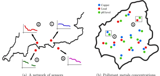
Accounting for dependencies between related processes has important applica-tions in several areas. In sensor networks, for example, missing signals from certain sensors may be predicted by exploiting their correlation with observed signals acquired from other sensors (Osborne et al., 2008), as shown in figure 1.1(a). Figure 1.1(a) represents a sketch of the south coast of England, where several sensors (the red dots in the figure), that keep track of different environ-mental variables, such as temperature and air pressure, have been placed along the coastline. In a normal scenario, we have access to the readings of all these devices at all time instants. However, at some random points in time, a num-ber of sensors can fail or segments of the sensor network can suffer disruptions, rendering inaccessible the information of certain environmental variables. Given that the sensors are located sufficiently close to each other and many of them make similar readings, we can make use of the signals obtained from the unbro-ken sensors (in figure 1.1(a), sensors b, c and d) to predict the missing signals for the broken ones (in figure 1.1(a), sensor a).
Ingeostatistics, predicting the concentration of heavy pollutant metals, which are expensive to measure, can be done using inexpensive and oversampled variables as a proxy (Goovaerts, 1997). Figure 1.1(b) illustrates a region of the Swiss Jura, for which we would like to know when the concentration of certain heavy metals, goes beyond a toxic threshold that can be risky for human health. It is usually cheaper to measure the level of pH in the soil (the green dots in the figure) than the concentration of Copper or Lead (the blue and read dots in the figure). We can exploit the correlations between the metals and pH level learned from different locations to predict, for example, the value of Lead in input location a,
a c d
b
(a) A network of sensors
b
a
(b) Pollutant metals concentrations Figure 1.1: Examples of the type of problems that we consider in this thesis.
(a) Walking movement with missing poses (b) Frames have been filled with plausible poses Figure 1.2: An example of a walking exercise. In 1.2(a), there are missing poses that are filled in 1.2(b).
shown in figure 1.1(b) or the value of Copper in input location b.
In computer graphics, a common theme is the animation and simulation of phys-ically plausible humanoid motion. As shown in figure 1.2(a), given a set of poses that delineate a particular movement (for example, walking), we are faced with the task of completing a sequence by filling in the missing frames with natural-looking poses, as in figure 1.2(b). Human movement exhibits a high-degree of correlation. Think, for example, of the way we walk. When moving the right leg forward, we unconsciously prepare the left leg, which is currently touching the ground, to start moving as soon as the right leg reaches the floor. At the same time, our hands move synchronously with our legs. We can exploit these im-plicit correlations for predicting new poses and for generating new natural-looking walking sequences.
access to secondary information (in the geostatistics example, pH levels) and consequently employ models that make predictions individually for each variable (Copper and Lead). However, these examples share an underlying principle: it is possible to exploit the interaction between the different variables to improve their joint prediction. Within the machine learning community this type of modeling is sometimes referred to asmultitask learning. The idea in multitask learning is that information shared between different tasks can lead to improved performance in comparison to learning the same tasks individually. It also refers to systems that learn by transferring knowledge between different domains, for example, what can we learn about running through seeing walking? Therefore it is also known as “transfer learning” (Thrun, 1996; Caruana, 1997; Bonilla et al., 2008).
There are plenty of methods in the literature that have been used to approach the type of problems we have described, including neural networks (Caruana, 1997), Bayesian neural networks (Bakker and Heskes, 2003), Dirichlet process priors (Xue et al., 2007) and support vector machines (Evgeniou et al., 2005). Essentially, this sort of problems conform to a multivariate regression analysis.1 If we assume that the variables are independent given the inputs, then, the simul-taneous regression transforms to a series of single variable regression problems. Nowadays, the most established technology for univariate regression, within the machine learning community, corresponds to Gaussian process (GP) regression (Rasmussen and Williams, 2006).
A Gaussian process specifies aprior distributionover functionsf(x), withx∈ <p. The distribution is defined in terms of a positive semidefinite function k(x,x0), known as the covariance function, that encodes the degree of similarity or corre-lation between f(x) and f(x0) as a function of the inputs x and x0. Covariance functions for single outputs are widely studied in machine learning (see, for ex-ample, Rasmussen and Williams, 2006) and some examples include the squared-exponential or the Mat´ern class of covariance functions. From a Bayesian statis-tics point of view, the Gaussian process specifies our prior beliefs about the prop-erties of the functions we are modeling. Our beliefs are updated in the presence of data by means of a likelihood function, that relates our prior assumptions to the actual observations, leading to an updated distribution, theposterior distribution, that can be used, for example, for predicting test cases.
1Multivariate problems are also known as multivariable, multiple output or multiple response problems.
work for modeling correlated outputs. The main challenge is the definition of a covariance function that encodes not only the degree of correlation of a process fd(x) as function of the input x, but, concomitantly, expresses the correlation between two different processes fd(x) and fd0(x), for d 6= d0. Importantly, the
covariance function must be valid, that is, positive semidefinite.
Much of the common practice in univariate Gaussian process regression, as it is done today in machine learning, has been rigorously systematized in Rasmussen and Williams (2006). Except for some isolated attempts, the counterpart for the multivariate case is yet to be written. In this thesis, we introduce some ideas towards that direction, from both theoretical and applied perspectives.
Outline of the thesis and contributions
One of the paradigms that has been considered for extending Gaussian processes to the multivariable scenario (Teh et al., 2005; Osborne et al., 2008; Bonilla et al., 2008) is known in the geostatistics literature as thelinear model of coregionaliza-tion (LMC) (Journel and Huijbregts, 1978; Goovaerts, 1997). In the LMC the covariance function is expressed as the sum of products betweencoregionalization matrices and a set of underlying covariance functions. The correlations across the outputs are expressed in the coregionalization matrices, while the underly-ing covariance functions express the correlation between different data points in terms of the input vectors.
An alternative approach to constructing covariance functions for multiple outputs employsprocess convolutions (PC). To obtain a PC in the single output case, the output of a given process is convolved with a smoothing kernel function. For example, a white noise process may be convolved with a smoothing kernel to obtain a covariance function (Barry and Ver Hoef, 1996). Ver Hoef and Barry (1998) noted that if a single input process was convolved with different smoothing kernels to produce different outputs, then correlation between the outputs could be expressed. This idea was introduced to the machine learning audience by Boyle and Frean (2005a).
Although these base processes have been considered almost exclusively as white noise Gaussian processes, in this thesis we allow the bases processes to be Gaus-sian processes with more general covariance functions. The first contribution
in this thesis is to develop a unifying model for the covariance function for mul-tiple outputs that contains the linear model of coregionalization and the process convolution as special cases. We refer to this model as the convolved multiple output covariance (CMOC). In chapter 2, we arrive at this covariance function by building upon previous work in the linear model of coregionalization literature and the process convolution literature.
The convolved multiple output covariance is obtained by convolving covariance functions with smoothing kernels. Usually it is difficult to specify in advance a functional form for the smoothing kernel that results in meaningful covariance functions, in the sense that the resulting multiple output covariance can represent important features of the data. Drawing connections with the theory of differ-ential equations as in Lawrence et al. (2007), our second contribution is that we develop a general framework in which the smoothing kernels correspond to the Green’s function associated to the differential equations used to describe the system. In chapter 3, we develop this idea under the name oflatent force models. A Gaussian process is a nonparametric technique and due to this nonparametric nature it carries the cross of being computationally expensive to use in prac-tice. The expensive steps are related to the successive inversion of the covariance matrix computed from the covariance function of the Gaussian process. In the multiple output case, the computational complexity grows as O(D3N3), where N is the number of observations per output and D is the number of outputs. Our third and fourth contributions are the development of efficient approx-imation techniques that reduce computational complexity to O(DNK2), where K is a user-specified parameter. In the third contribution, we develop reduced rank approximations for the covariance matrix of the full Gaussian process by exploiting different conditional independence assumptions in the likelihood func-tion. In the fourth contribution, we introduce the concept of inducing function. An inducing function acts as a smooth surrogate for white noise processes, when these processes are used as base functions in the CMOC. Embedding these in-ducing functions in a variational framework, replicating ideas presented in Titsias (2009), we develop an efficient approximation that behaves as a lower bound of the marginal likelihood of the full multivariate Gaussian process. Both contributions and the relationships between them are presented in chapter 4.
Finally, in chapter 5 we present our fifth contribution. We propose a novel model that allows discrete changes in the parameter space of the smoothing kernel
focus is to develop a latent force model in which the parameters of the multivariate covariance change as a function of the input variable. Thus, the model obtained allows for the description of highly nonstationary multivariate time series courses.
How to read this thesis
This thesis follows the Alternative Format Thesis allowed by the University of Manchester thesis submission regulations,2 that consents to incorporate sections that are in a format suitable for submission for publication in a peer-reviewed journal. The way in which the thesis has been developed is as follows. The main document serves as a backbone of a series of contributions already published at the Annual Conference on Neural Information Processing Systems (NIPS), the International Conference on Artificial Intelligence and Statistics (AISTATS), a journal paper at theJournal of Machine Learning Researchand a technical report appearing in ´Alvarez et al. (2009). Each chapter includes in the introduction a remark that explains what sections of the chapter have been published. We then describe the theory involved in that chapter and include an experiment that illustrates the main ideas developed. At the end of each chapter, we comment about further experiments that accompany the theory and that are found in the publications. Reprints of the publications are attached at the end of the document.
We refer to the publications using the numbers in the list of publications of the following section. So for example, we will use expressions like “in publicationiv” to refer to the publication [iv] in the list below.
List of publications
The main contributions in the thesis have been presented in the following publi-cations and a submitted paper.
[i] Mauricio A. ´Alvarez and Neil D. Lawrence (2008): Sparse Convolved Gaus-sian Processes for Multi-output Regression, in D. Koller and D. Schuurmans and Y. Bengio and L. Bottou (Eds), Advances in Neural Information Pro-cessing Systems 21, pp 57-64, 2009.
[ii] Mauricio A. ´Alvarez, David Luengo and Neil D. Lawrence. Latent Force Models, in D. van Dyk and M. Welling (Eds.), Proceedings of The Twelfth International Conference on Artificial Intelligence and Statistics (AISTATS) 2009, JMLR: W&CP 5, pp. 9-16, Clearwater Beach, Florida, April 16-18, 2009.
[iii] Mauricio A. ´Alvarez, David Luengo, Michalis K. Titsias and Neil D. Lawrence (2010): Efficient Multioutput Gaussian Processes through Variational In-ducing Kernels, in Y. Whye Teh and M. Titterington (Eds.), Proceedings of The Thirteenth International Conference on Artificial Intelligence and Statistics (AISTATS) 2010, JMLR: W&CP 9, pp. 25-32, Chia Laguna Re-sort, Sardinia, Italy, May 13-15, 2010.
[iv] Mauricio A. ´Alvarez, Jan Peters, Bernhard Sch¨olkopf and Neil D. Lawrence (2011): Switched latent force models for movement segmentation, in J. Shawe-Taylor, R. Zemel, C. Williams and J. Lafferty (Eds), Advances in Neural Information Processing Systems 23, pp 55-63, 2011. See also the supplementary material accompanying the publication.
[v] Mauricio A. ´Alvarez and Neil D. Lawrence (2011): “Computationally Effi-cient Convolved Multiple Output Gaussian Processes”,Journal of Machine Learning Research 12, pp 1425–1466.
In all publications, ´Alvarez had the main responsibility in writing a first draft of the paper and developing the software. Revisions of the writing were incorporated by the coauthors directly or by ´Alvarez after discussions with the other authors. For publication ii, Luengo developed the analytical expression for the covariance function of the second order latent force model. For publication iii, Luengo developed the covariance function for a latent force model driven by white noise and Titsias helped with the description of the variational framework. Publication iv was supervised by Peters, Sch¨olkopf and Lawrence. All the other publications were supervised by Lawrence.
Covariance functions for
multivariate regression
In chapter 1, we discussed applications of multivariate regression that are en-countered in machine learning problems, including multitask learning (see Bonilla et al., 2008, for example). In geostatistics these models are used for jointly pre-dicting the concentration of different heavy metal pollutants (Goovaerts, 1997). In statistics more researchers are becoming interested in emulation of multiple output simulators (see Higdon et al., 2008; Rougier, 2008; Conti and O’Hagan, 2010, for example). In this chapter we provide a general review of structured covariance/kernel functions for multiple outputs.
There is a huge amount of work in geostatistics focused on constructing valid covariance functions for predicting spatial varying data. The basic approach is based on the so called “Linear Model of Coregionalization” (Journel and Hui-jbregts, 1978; Goovaerts, 1997). Similar methods have been suggested in several machine learning and statistics related papers, including special type of kernels proposed as a generalization of the regularization theory to vector-valued func-tions. We show how some of those methods can be seen as particular cases of the linear model of coregionalization.
An alternative approach for constructing the covariance function involves a mov-ing average construction in the form of “Process Convolutions” (Ver Hoef and Barry, 1998; Higdon, 2002). In a process convolution a latent process is convolved with output-specific smoothing kernels to produce a valid covariance. The latent process is usually assumed to be a white noise process. If the latent process fol-lows a Gaussian process with general covariance function, we will see that the
2.1. KERNELS FOR MULTIPLE OUTPUTS
linear model of coregionalization and the process convolution framework can be interpreted as particular cases of this moving-average construction. We refer to this covariance as the “Convolved Multiple Output Covariance” (CMOC). Having firstly presented alternatives for constructing multivariate kernel func-tions, we then embed these kernels in a Gaussian process prior and explain two important aspects of multivariate Gaussian process regression, namely, how to perform parameter estimation and prediction for test data. We also briefly re-view how parameter estimation and prediction is done in research areas such as geostatistics and statistics.
The chapter is organized as follows. In section 2.1, different methods for con-structing the kernel for multiple outputs are reviewed, including the linear model of coregionalization and process convolutions. We then employ the defined co-variances for multivariate regression with Gaussian process priors in section 2.2. Finally, in section 2.3, we present an example of multivariate regression in gene expression data.
Remark. In publicationv, we introduced the main idea that appears in section 2.1 and that is the motivation for this chapter. Detailed analysis of related work, including the linear model of coregionalization in computer emulation, is new, though. The example of section 2.3 also appears in publication v.
2.1 Kernels for multiple outputs
In geostatistics, prediction over multivariate output data is known as cokriging. Geostatistical approaches to multivariate modelling are mostly formulated around the “linear model of coregionalization” (LMC, see, e.g., Journel and Huijbregts, 1978; Wackernagel, 2003). We will first consider this model and discuss how several recent models proposed in the machine learning and statistics literature are special cases of the LMC, including approaches to constructing “multitask” kernels in machine learning introduced from the perspective of regularization theory (Evgeniou and Pontil, 2004). We also review different alternatives for the moving average construction of the covariance function, under the generic name of process convolutions and introduce the model for the covariance function that is used in the thesis.
2.1.1 The linear model of coregionalization
In the linear model of coregionalization, the outputs are expressed as linear com-binations of independent random functions. This is done in such a way that ensures that the resulting covariance function (expressed jointly over all the out-puts and the inout-puts) is a valid positive semidefinite function. Consider a set of D variables {fd(x)}D
d=1 with x ∈ <p. In the LMC, each variable fd is expressed as (Journel and Huijbregts, 1978)
fd(x) = Q
X
q=1
ad,quq(x) +µd,
where µd represents the mean of each process fd(x) and the functions uq(x), with q = 1, . . . , Q, have mean equal to zero and covariance cov[uq(x), uq0(x0)] =
kq(x,x0)δ
q,q0, where δq,q0 is the Kronecker delta (δq,q0 = 1 if q = q0 and δq,q0 = 0
if q 6=q0). Therefore, the processes {uq(x)}Q
q=1 are independent. We will assume that µd = 0 for all outputs, unless it is stated otherwise. Some of the basic processes uq(x) and uq0(x0) can have the same covariance kq(x,x0), kq(x,x0) =
kq0(x,x0) while remaining orthogonal. A similar expression for {fd(x)}D
d=1 can be written grouping the functions uq(x) which share the same covariance (Journel and Huijbregts, 1978; Goovaerts, 1997)
fd(x) = Q X q=1 Rq X i=1 ai d,quiq(x), (2.1)
where the functions ui
q(x), with q = 1, . . . , Q and i = 1, . . . , Rq, have mean equal to zero and covariance cov[ui
q(x), ui
0
q0(x0)] = kq(x,x0)δi,i0δq,q0. Expression
(2.1) means that there are Q groups of functions ui
q(x) and, within each group, functionsui
q(x) share the same covariance, but are independent. We assume that the processes fd(x) are second-order stationary.1 The cross covariance between any two functions fd(x) and fd0(x) is given in terms of the covariance functions
1The stationarity condition is introduced so that the prediction stage can be realized through a linear predictor using a single realization of the process (Cressie, 1993). Implicitly, ergodicity is also assumed. For nonstationary processes, description is done in terms of the so called
2.1. KERNELS FOR MULTIPLE OUTPUTS for ui q(x) cov[fd(x), fd0(x+h)] = Q X q=1 Q X q0=1 Rq X i=1 Rq X i0=1 ai d,qai 0 d0,q0cov[uiq(x), ui 0 q0(x+h)],
withh=x−x0 being the lag vector. We refer to the covariance cov[f
d(x), fd0(x+
h)] as kfd,fd0(h). Due to the independence of the functions u i q(x), the above expression reduces to kfd,fd0(h) = Q X q=1 Rq X i=1 ai d,qaid0,qkq(h) = Q X q=1 bqd,d0kq(h), (2.2) with bqd,d0 = PRq
i=1aid,qaid0,q. For theD outputs, equation (2.1) can be expressed in
matrix form as f(x) = Q X q=1 Aquq(x),
where, for each x, f(x) = [f1(x), . . . , fD(x)]>, Aq ∈ <D×Rq is a matrix with entries ai
d,q and uq(x) = [u1q(x), . . . , uRqq(x)]>. The covariance function foruq(x) is
cov[uq(x),uq0(x+h)] = kq(h)IR
qδq,q0, where IRq ∈ <R
q×Rq is the identity matrix.
The covariance function for the outputs is then given as cov[f(x),f(x+h)] = E Q X q=1 Aquq(x) Q X q0=1 Aq0uq0(x+h) !> = Q X q=1 Q X q0=1 AqEuq(x)u>q0(x+h) A> q0 = Q X q=1 AqA> qkq(h). (2.3)
Equation (2.3) can be written as Kf,f(h) = Q X q=1 Bqkq(h), (2.4)
where Kf,f(h) = cov[f(x),f(x+h)] and Bq =AqA>q, with Bq ∈ <D×D is known as the coregionalization matrix. In general, we denote the covariance of f(x) as Kf,f(x,x0) = cov[f(x),f(x0)]. For the stationary case, it reduces to Kf,f(h). The elements of eachBq are the coefficientsbqd,d0 appearing in equation (2.2). The
covariance functionKf,f(h) is positive semidefinite as long as the coregionalization matricesBq are positive semi-definite andkq(h) is a valid covariance function. By definition, matricesBqfulfill the positive semidefiniteness requirement and several models for the covariance function kq(h) can be used, for example the squared exponential covariance function, the Mat´ern class of covariance functions, among others (see Rasmussen and Williams, 2006, chap. 4).
Equation (2.1) can be interpreted as a nested structure (Wackernagel, 2003) in which the outputsfd(x) are first expressed as a linear combination of spatially un-correlated processesfd(x) =PQq=1fdq(x),with E[fdq(x)] = 0 and cov[fdq(x), fq
0
d0(x+
h)] = bqd,d0kq(h)δq,q0. At the same time, each process fq
d(x) can be represented as a set of uncorrelated functions weighted by the coefficients ai
d,q, fdq(x) =
PRq
i=1aid,quiq(x) where again, the covariance function foruiq(x) is kq(h).
The linear model of coregionalization represents the covariance function as the sum of the products of two covariance functions. One of the covariance functions models the dependence between the functions, independently of the input vector x, this is given by the coregionalization matrix Bq, whilst the other covariance function models the input dependence, independently of the particular set of functions fd(x), this is the covariance function kq(h). In equation (2.4), the output covariance for a particular value of the lag vector h, is represented as a weighted sum of the same set of coregionalization matricesBq, where the weights depend on the inputx, given by the factorskq(h).
For a numberN of input vectors, letfdbe the vector of values from the outputd evaluated at X={xn}Nn=1. If each output has the same set of inputs the system is known as isotopic. In general, we can allow each output to be associated with a different set of inputs, X(d) = {x(d)
n }Nn=1d , this is known as heterotopic.2 For 2These names come from geostatistics (Wackernagel, 2003). Heterotopic data is further classified intoentirely heterotopic data, where the variables have no sample locations in common,
2.1. KERNELS FOR MULTIPLE OUTPUTS
notational simplicity, we restrict ourselves to the isotopic case, but our analysis can be easily used for heterotopic setups. The covariance matrix forfdis obtained by expressing equation (2.2) as cov[fd,fd0] = Q X q=1 Rq X i=1 ai d,qaid0,qKq = Q X q=1 bqd,d0Kq, (2.5)
where Kq∈ <N×N has entries kq(h), for the different values that h may take for the particular set X. Define f as f = [f>
1 , . . . ,fD>]>. The covariance matrix for f in terms of equation (2.5) can be written as
Kf,f = Q
X
q=1
Bq⊗Kq, (2.6)
with the symbol⊗representing the Kronecker product between matrices (Brookes, 2005).
Intrinsic coregionalization model
A simplified version of the LMC, known as the intrinsic coregionalization model (ICM) (see Goovaerts, 1997), assumes that the elements bq
d,d0 of the
coregional-ization matrix Bq can be written as bqd,d0 = υd,d0bq. In other words, as a scaled
version of the elementsbqwhich do not depend on the particular output functions fd(x). Using this form for bqd,d0, equation (2.2) can be expressed as
cov[fd(x), fd0(x0)] = Q X q=1 υd,d0bqkq(x,x0) =υd,d0 Q X q=1 bqkq(x,x0) =υd,d0k(x,x0), where k(x,x0) = PQ
q=1bqkq(x,x0) is an equivalent covariance function. The co-variance matrix for f takes the form
Kf,f =Υ⊗K, (2.7)
where Υ ∈ <D×D, with entries υ
d,d0, and K= PQ
q=1bqKq is an equivalent valid covariance matrix.
and partially heterotopic data, where the variables share some sample locations. In machine learning, the partially heterotopic case is sometimes referred to asasymmetric multitask learning
The intrinsic coregionalization model can also be seen as a linear model of core-gionalization where we haveQ= 1. In such case, equation (2.6) takes the form
Kf,f =A1A>1 ⊗K1 =B1⊗K1, (2.8)
where the coregionalization matrix B1 has elements b1d,d0 = PR1
i=1aid,1aid0,1. The
value ofR1 determines the rank of the matrix B1.
As pointed out by Goovaerts (1997), the ICM is much more restrictive than the LMC since it assumes that each basic covariance kq(x,x0) contributes equally to the construction of the autocovariances and cross covariances for the outputs. However, for inference purposes, the inverse of the covariance matrix Kf,f can be computed using the properties of the Kronecker product (as along as the input space follows the isotopic configuration) reducing the computational complexity involved when compared to the matrix inversion of the full covariance matrixKf,f obtained from LMC. This property is employed by Rougier (2008) to speed-up the inference process in an emulator for multiple outputs. First, it assumes that the multiple output problem can be seen as a single output problem considering the output index as another variable of the input space. Then, the new output fD(ex), withex∈ <
p×
D andDthe set D={1, . . . , D}, is expressed as a weighted sum of Q deterministic regressors, {gq(ex)}
Q
q=1, plus a Gaussian error term e(ex)
with covariance κ(xe,ex
0). The set of regressors explain the mean of the output process, while the Gaussian error term explains the variance in the output. Both, the set of regressors and the covariance for the error, are assumed to be separable in the input space, this is, each regressor gq(x)e ≈ gq(x)gq(d) and the covariance
κ(ex,xe
0) = κ(x,x0)κ(d, d0). For isotopic spaces (Rougier (2008) refers to this condition as regular outputs, meaning outputs that are evaluated at the same set of inputsX), the mean and covariance for the outputfD(ex), can be obtained
through Kronecker products for the regressors and the covariances involved in the error term. For inference, the inversion of the necessary terms is accomplished using properties of the Kronecker product. We will see in the next section that the model that replaces the set of outputs for a single output as described before, can be seen as a particular case of the intrinsic coregionalization model (Conti and O’Hagan, 2010).
It can be shown that if the outputs are considered to be noise-free, prediction using the intrinsic coregionalization model under an isotopic data case is equivalent to independent prediction over each output (Helterbrand and Cressie, 1994). This
2.1. KERNELS FOR MULTIPLE OUTPUTS
circumstance is also known as autokrigeability (Wackernagel, 2003).
Linear Model of Coregionalization in Machine Learning and Statistics The linear model of coregionalization has already been used in machine learning in the context of Gaussian processes for multivariate regression, and regularization theory for multitask learning. It has also been used in statistics for computer emulation of expensive multivariate computer codes.
Before looking at related work, let us define the parameter space for the LMC. The set of parameters in the LMC includes the coregionalization matrices, {Bq}Qq=1, and the parameters associated to the basic covariances kq(x,x0), that we denote here as ψq, also called hyperparameters. We use θLMC = {{Bq}Qq=1,{ψq}Qq=1} to denote the whole set of parameters involved in the LMC or θICM = {B1,ψ1} if
Q= 1.
As we have seen before, the linear model of coregionalization imposes the corre-lation of the outputs explicitly through the set of coregionalization matrices. A recurrent idea in the early days of Gaussian processes for multi-output modeling, within the machine learning literature, was based on the intrinsic coregionaliza-tion model and assumedB1 =ID. In other words, the outputs were considered to be conditionally independent given the parameters ψ1. Correlation between the outputs was assumed to exist implicitly by imposing the same set of hyperparam-eters ψ1 for all outputs, and estimating those parameters, or directly the kernel matrix K1, using data from all the outputs (Minka and Picard, 1999; Lawrence and Platt, 2004; Yu et al., 2005).
In this section, we review more recent approaches for multiple output modeling that are different versions of the linear model of coregionalization.
Semiparametric latent factor model. The semiparametric latent factor model (SLFM) proposed by Teh et al. (2005) turns out to be a simplified version of equa-tion (2.6). In particular, if Rq = 1 (see equation (2.1)), we can rewrite equation (2.6) as Kf,f = Q X q=1 aqa> q ⊗Kq,
where aq ∈ <D×1 with elements {ad,q}D
d=1 and q fixed. With some algebraic manipulations, that exploit the properties of the Kronecker product, we can write
Kf,f = Q
X
q=1
(aq⊗IN)Kq(a>q ⊗IN) = (Ae ⊗IN)K(e Ae>⊗IN),
where Ae ∈ <D×Q is a matrix with columns aq, and Ke ∈ <QN×QN is a block
diagonal matrix with blocks given by Kq.
The functions uq(x) are considered to be latent factors and the semiparametric name comes from the fact that it is combining a nonparametric model, this is a Gaussian process, with a parametric linear mixing of the functions uq(x). The kernel for each basic processq,kq(x,x0), is assumed to be of Gaussian type with a different length scale per input dimension. For computational speed up the informative vector machine (IVM) is employed (Lawrence et al., 2003).
Multi-task Gaussian processes. The intrinsic coregionalization model has been employed by Bonilla et al. (2008) for multitask learning. We refer to this approach as multi-task Gaussian processes (MTGP). The covariance matrix is expressed as Kf,f(x,x0) = Kfk(x,x0), with Kf being constrained positive semi-definite and k(x,x0) a covariance function over inputs. It can be noticed that this expression is similar to the one in (2.7), when it is evaluated for x,x0 ∈X. In Bonilla et al. (2008), Kf (equal to Υ in equation (2.7) or B1 in equation (2.8)) expresses the correlation between tasks or inter-task dependencies, and it is represented through a probabilistic principal component analysis (PPCA) model. In turn, the spectral factorization in the PPCA model is replaced by an incomplete Cholesky decomposition to keep numerical stability, so that Kf ≈
e
LLe>, where Le ∈ <D×R1. The authors also refer to the autokrigeability effect
as the cancellation of inter-task transfer (Bonilla et al., 2008). An application of MTGP for obtaining the inverse dynamics of a robotic manipulator was presented in Chai et al. (2009).
Multi-output Gaussian processes. The intrinsic coregionalization model has been also used by Osborne et al. (2008). Matrix Υ in expression (2.7) is assumed to be of the spherical parametrisation kind, Υ = diag(e)S>Sdiag(e), where e gives a description for the length scale of each output variable and S is an upper triangular matrix whose i-th column is associated with particular
2.1. KERNELS FOR MULTIPLE OUTPUTS
spherical coordinates of points in <i (for details see Osborne and Roberts, 2007, sec. 3.4). Function k(x,x0) is represented through a Mat´ern kernel, where dif-ferent parametrisations of the covariance allow the expression of periodic and non-periodic terms. Sparsification for this model is obtained using an IVM style approach.
Multi-task kernels in regularization theory. Kernels for multiple outputs have also been studied in the context of regularization theory. The approach is based mainly on the definition of kernels for multitask learning provided in Evgeniou and Pontil (2004); Micchelli and Pontil (2005); Evgeniou et al. (2005). The derivation is based on the theory of kernels for vector-valued functions. Ac-cording to Evgeniou et al. (2005), the following lemma can be used to construct multitask kernels,
Lemma. If G is a kernel on T × T and, for every d ∈ D there are prescribed mappings Φd:X → T such that
kd,d0(x,x0) = k((x, d),(x0, d0)) = G(Φd(x),Φd0(x0)), x,x0 ∈ <p, d, d0 ∈D,
then k(·) is a multitask or multioutput kernel.
A linear multitask kernel can be obtained if we set T =<m, Φ
d(x) = Cdxwith Φd∈ <m and G:<m× <m→ < as the polynomial kernelG(z,z0) = (z>z0)nwith n = 1, leading to kd,d0(x,x0) = x>C>dCd0x0. The lemma above can be seen as
the result of applying kernel properties to the mapping Φd(x) (see Genton, 2001, pag. 2). Notice that this corresponds to a generalization of the semiparametric latent factor model where each output is expressed through its own basic process acting over the linear transformation Cdx, this is, ud(Φd(x)) = ud(Cdx). In general, it can be obtained from fd(x) = PD
q=1ad,quq(Φq(x)), where ad,q = 1 if d=q or zero, otherwise.
Computer emulation. A computer emulator is a statistical model used as a surrogate for a computationally expensive deterministic model or computer code, also known as simulator. Gaussian processes have become the preferred statis-tical model among computer emulation practitioners (for a review see O’Hagan, 2006). Different Gaussian process emulators have been recently proposed to deal with several outputs (Higdon et al., 2008; Conti and O’Hagan, 2010; Rougier, 2008). In Higdon et al. (2008), the linear model of coregionalization was used to
model images representing the evolution of the implosion of steel cylinders after using TNT, and obtained employing the so called Neddemeyer simulation model (see Higdon et al., 2008, for further details). The input variable x represents parameters of the simulation model, while the output is an image of the radius of the inner shell of the cylinder over a fixed grid of times and angles. In the version of the LMC that the authors employed, Rq = 1, and the Q vectors aq were obtained as the eigenvectors of a PCA decomposition of the set of training images.
In Conti and O’Hagan (2010), the intrinsic coregionalization model is employed for emulating the response of a vegetation model called the Sheffield Dynamic Global Vegetation Model (SDGVM) (Woodward et al., 1998). Authors refer to the ICM as the Multiple-Output (MO) emulator. The inputs to the model are variables related to broad soil, vegetation and climate data, while the outputs are time series of the index Net Biome Productivity (NBP) measured at different sites. The NBP index accounts for the residual amount of carbon at a vegetation site after some natural processes have taken place. In the paper, the authors as-sume that the outputs correspond to the different sampling time points, so that D =T, being T the number of time points, while each observation corresponds to a spatial sampling site.
As we mentioned before, Rougier (2008) introduces an emulator for multiple-outputs that assumes that the set of output variables can be seen as a single variable while augmenting the input space with an additional index over the out-puts. In other words, it considers the output variable as an input variable. Conti and O’Hagan (2010) refer to the model in Rougier (2008) as the Time input (TI) emulator. They discussed how the TI model turns out to be a particular case of the MO model, by using a squared-exponential kernel (see Rasmussen and Williams, 2006, chapter 4) for computing the entries in the coregionalization matrix B1.
2.1.2 Process convolutions for multiple outputs
The approaches introduced above involve some form of instantaneous mixing through a linear weighted sum of independent processes to construct correlated processes. By instantaneous mixing we mean that the output functionf(x) eval-uated at the input point x only depends on the values of the latent functions {uq(x)}Qq=1 at the same input x. Instantaneous mixing has some limitations. If
2.1. KERNELS FOR MULTIPLE OUTPUTS
we wanted to model two output processes in such a way that one process was a blurred version of the other, we cannot achieve this through instantaneous mix-ing. We can achieve blurring through convolving a base process with a smoothing kernel.3 If the base process is a Gaussian process, it turns out that the convolved process is also a Gaussian process. We can therefore exploit convolutions to con-struct covariance functions (Barry and Ver Hoef, 1996; Ver Hoef and Barry, 1998; Higdon, 1998, 2002). A recent review of several extensions of this approach for the single output case is presented in Calder and Cressie (2007). Applications include the construction of nonstationary covariances (Higdon, 1998; Higdon et al., 1998; Fuentes, 2002a,b; Paciorek and Schervish, 2004) and spatiotemporal covariances (Wikle et al., 1998; Wikle, 2002, 2003).
We will first introduce the idea of moving average construction for multivariate responses as it has traditionally been presented in the statistics and geostatis-tics literature (Ver Hoef and Barry, 1998; Ver Hoef et al., 2004; Higdon, 2002). They normally consider convolutions between kernels and white Gaussian noise processes. We then describe the covariance model used in the thesis, that allows for convolutions of kernels with more general Gaussian processes. A similar idea was presented by Fuentes (2002a,b) using discrete convolutions for developing nonstationary covariances, in the single output case.
Consider again a set ofDfunctions{fd(x)}D
d=1. Each function could be expressed through a convolution integral between a kernel, {Gd(x)}D
d=1, and a function {rd(x)}D d=1, fd(x) = Z X Gd(x−z)rd(z)dz.
For the integral to exist, it is assumed that the kernel Gd(x) is a continuous function with compact support (H¨ormander, 1983) or square-integrable (Ver Hoef and Barry, 1998; Higdon, 2002). The kernel Gd(x) is also known as the moving average function (Ver Hoef and Barry, 1998) or the smoothing kernel (Higdon, 2002).
The function rd(x) is given by rd(x) = ρdwd(x) + adu(x). It is composed of two elements: a white Gaussian noise random process associated to each output,
wd(x), with mean zero and variance one, and a white Gaussian noise random
3We use kernel to refer to both reproducing kernels and smoothing kernels. Reproducing kernels are those used in machine learning that conform to Mercer’s theorem. Smoothing kernels are functions which are convolved with a signal to create a smoothed version of that signal.
process that is common to all outputs, u(x), also with mean zero and variance one. We can choose ρd, such that the variance of rd(x) be equal to one. For example, in Ver Hoef and Barry (1998),ρd=p1−a2d. The processes{wd(x)}Dd=1 and u(x) are assumed to be independent.
The cross-covariance between fd(x) and fd0(x0) is then given by
cov [fd(x), fd0(x0)] = E Z X Gd(x−z)rd(z)dzZ X Gd0(x0−z0)rd0(z0)dz0 =Z X Z X Gd(x−z)Gd0(x0−z0) E [rd(z)rd0(z0)] dz0dz = covu[fd(x), fd0(x0)] + covw[fd(x), fd0(x0)]δd,d0,
where the subscripts u and w appearing in the covariance operator, emphasize the components of rd(x) and rd0(x) involved in the covariance expression. We
refer to cov [fd(x), fd0(x0)] askf d,fd0(x,x 0), cov u[fd(x), fd0(x0)] asku fd,fd0(x,x 0) and covw[fd(x), fd0(x0)] as kw fd,fd0(x,x 0). The covariancesku fd,fd0(x,x 0) andkw fd,fd0(x,x 0) are given as ku fd,fd0(x,x 0) = a dad0 Z X Gd(x−z)Gd0(x0 −z)dz (2.9) kw fd,fd(x,x 0) = ρ2 d Z X Gd(x−z)Gd(x0−z)dz.
With the equations above, we can indirectly specify a functional form for the co-variancekfd,fd0(x,x
0) through a particular choice of the smoothing kernelsGd(x). The smoothing kernels are usually parameterized functions and we refer to these parameters asθPC ={θGd}Dd=1, where the subscript PC stands for process convo-lution. Under the above construction, the covariance function for the vectorf(x) is positive semidefinite, for any fixed values of x=xi and x0 =xj.
In Ver Hoef and Barry (1998), the input space over which the integrals are com-puted is X =<p. Higdon (2002) depicted a similar construction to the one pre-sented above, but assuming that the functions rd(x) only included the common component u(x), so that rd(x) = r(x) = u(x). The input space is partitioned into disjoint subsets X =TD
d=0Xd, and the latent process u(x) is assumed to be independent on these separate subspaces. Each function fd(x) is expressed by
fd(x) =
Z
Xd∪X0
2.1. KERNELS FOR MULTIPLE OUTPUTS
The functions fd(x) and fd0(x) are dependent withinX0, but independent within
Xd and Xd0.
The approach described so far was introduced to the machine learning community with the name of “Dependent Gaussian Processes” (DGP) by Boyle and Frean (Boyle and Frean, 2005a,b) and further developed in Boyle (2007). Similar to Ver Hoef and Barry (1998), the input space is again X = <p. The components of the function rd(x), wd(x) and u(x) are considered independently (ρd and ad are assumed to be one), and additional moving average functions{Hd(x)}D
d=1 are convolved with the processeswd(x) to allow for a different functional form for the covariance kfd,fd0(x,x
0) whend=d0. In this way each output fd(x) follows fd(x) = Z X Gd(x−z)u(z)dz+ Z X Hd(x−z)wd(z)dz, and the covariancekfd,fd0(x,x
0) is again given byku fd,fd0(x,x 0) pluskw fd,fd0(x,x 0)δ d,d0, where ku fd,fd0(x,x
0) follows equation (2.9), with a
d = 1 for all outputs, and kw fd,fd(x,x 0) is kw fd,fd(x,x 0) = Z X Hd(x−z)Hd(x0−z)dz. (2.10) Additional modeling flexibility is allowed if instead of using a single and common white noise processu(x), we consider a set ofQ independent and common white noise processes {uq(x)}Qq=1, with zero mean and variance equal to one. Then the outputs {fd(x)}D d=1 can be expressed as fd(x) = Q X q=1 Z X Gd,q(x−z)uq(z)dz+Z X Hd(x−z)wd(z)dz, leading to a covariance ku fd,fd0(x,x 0) given as ku fd,fd0(x,x 0) = Q X q=1 Z X Gd,q(x−z)Gd0,q(x0−z)dz. The covariance kw fd,fd(x,x
0) follows the same expression appearing in equation (2.10). The parameter vector for the DGP includes the parameters for the kernels {Gd,q(x)}D,Qd=1,q=1, {θGd,q}D,Qd=1,q=1, and the parameters for the kernels {Hd(x)}Dd=1, {θHd}Dd=1. We also denote this set of parameters jointly as θPC.
In Majumdar and Gelfand (2007), a different moving average construction for the covariance of multiple outputs was introduced. It is obtained as a convolution over covariance functions in contrast to the process convolution approach where the convolution is performed over processes. Assuming that the covariances in-volved are isotropic, Majumdar and Gelfand (2007) show that the cross-covariance obtained from
cov [fd(x+h), fd0(x)] = Z
X
kd(h−z)kd0(z)dz,
where kd(h) and kd0(h) are covariances associated to the outputs d and d0, lead
to a valid covariance function for the outputs {fd(x)}D
d=1. If we assume that the smoothing kernels are not only square integrable, but also positive definite functions, then the covariance convolution approach turns out to be a particular case of the process convolution approach (square-integrability might be easier to satisfy than positive definiteness).
When developing a covariance function for multivariable processes, our aim is to specify jointly the dependencies over the input spaceX and over the set of outputs D. We have seen how in the linear model of coregionalization this compound dependency is broken in two different components, the coregionalization matrices Bq, that specify dependencies in the set D independently of X, and the basic kernels kq(x,x0), specifying dependencies overX independently ofD. Therefore, the LMC assumption implies that all cross-covariances cov [fd(x), fd0(x0)] share
the same input dependencies that are allowed by kq(x,x0). For a large value of Q, the weighted sum of covariances kq(x,x0) might indirectly reflect the different levels of variation in the input space. However, a large value forQalso leads to a larger parameter space for the vectorθLMC, particularly when the system involves a large number of outputsD. In practice, though, one usually has prior knowledge about the diverse degrees of variation that the outputs have as functions ofxand, subsequently, selects a set of covariances {kq(x,x0)}Qq=1 that better reflects that amount of variation. On the other hand, the process convolution framework attempts to model the variance of the set of outputs by the direct association of a different smoothing kernel Gd(x) to each output fd(x). By specifying Gd(x), one can model, for example, the degree of smoothness and the length-scale that characterizes each output. If each output happens to have more than one degree of variation (marginally, it is a sum of functions of varied smoothness) one is
2.1. KERNELS FOR MULTIPLE OUTPUTS
faced with the same situation than in LMC, namely, the need to augment the parameter space θPC so as to satisfy a required precision. However, due to the local description of each output that the process convolution performs, it is likely that the parameter space θPC grows slower than the parameter space for LMC.
Here we have two methods that allows us to specify the degree of variation in each output fd(x) while leading to a valid covariance function for multiple outputs: globally, by means of Q underlying covariance functions kq(x,x0) via the linear model of coregionalization or locally, through a set of smoothing kernels Gd,q(x) by way of the process convolution framework.
In this thesis, we employ an extension of the process convolution framework that lies somewhere between the local and the global methods we described above. We refer to this extension as the “convolved multiple output covariance” (CMOC) In a similar way to the linear model of coregionalization, we consider Q groups of functions, where a particular group q has elements ui
q(z), for i = 1, . . . , Rq. Each member of the group has the same covariance kq(x,x0), but is sampled independently. Any output fd(x) is described by
fd(x) = Q X q=1 Rq X i=1 Z X Gi d,q(x−z)uiq(z)dz+wd(x) = Q X q=1 fdq(x) +wd(x), where fdq(x) = Rq X i=1 Z X Gi d,q(x−z)uiq(z)dz, (2.11) and {wd(x)}D
d=1 are independent Gaussian processes with mean zero and covari-ancekwd(x,x
0). We have included the superscript qforfq
d(x) in (2.11) to empha-size the fact that the function depends on the set of latent processes {ui
q(x)}Ri=1q . Notice that in the process convolution formulation, each function wd(x) was a part of rd(x) and led to the covariance kfwd,fd(x,x
0), which was a function of ei-ther Gd(x) or both Gd(x) and Hd(x). Here we allow the covariance kwd(x,x
0) to be any valid covariance function. Importantly, the latent functions ui
q(z) are Gaussian processes with general covariances kq(x,x0), in contrast to the process convolution framework is which they were assumed to be white noise Gaussian processes.
Under the same independence assumptions used in the linear model of coregion-alization, the covariance between fd(x) and fd0(x0) follows
kfd,fd0(x,x 0) = Q X q=1 kfq d,f q d0(x,x 0) +k wd(x,x 0)δ d,d0, (2.12) where kfq d,f q d0(x,x 0) = Rq X i=1 Z X Gi d,q(x−z) Z X Gi d0,q(x0 −z0)kq(z,z0)dz0dz. (2.13) SpecifyingGi
d,q(x−z) andkq(z,z0) in (2.13), the covariance for the outputsfd(x) can be constructed indirectly.
Notice that if the smoothing kernels are taken to be the Dirac delta function such thatGi
d,q(x−z) =aid,qδ(x−z),4 the double integral is easily solved and the linear model of coregionalization is recovered. On the other hand, if the latent processes ui
q(x) are white Gaussian noise processes with mean zero and variance one, we recover the process convolution formulation (with Rq = 1),
kfd,fd0(x,x 0) = Q X q=1 Z X Gd,q(x−z)Gd0,q(x0−z)dz+kw d(x,x 0).
As well as the covariance across outputs, the covariance between the latent func-tion, ui
q(z), and any given output, fd(x), can be computed, kfd,uiq(x,z) = cov fd(x), uiq(z) = Z X Gi d,q(x−z0)kq(z0,z)dz0. (2.14) The convolved multiple output covariance can also be seen as a dynamic version of the linear model of coregionalization: the latent functions are dynamically combined with the help of the kernel smoothing functions, as opposed to the static combination of the latent functions in the LMC case. We are interested in allowing the latent Gaussian processes ui
q(x) to go beyond the white noise assumption for different reasons. First, in several problems in systems biology, the latent functions represent physical quantities, for example, transcription factor 4We have slightly abused of the delta notation to indicate the Kronecker delta for discrete arguments and the Dirac function for continuous arguments. The particular meaning should be understood from the context.