journal homepage:
www.elsevier.com/locate/aml
Multi-innovation stochastic gradient algorithms for dual-rate sampled
systems with preload nonlinearity
✩Jing Chen
a
,
b
, Lixing Lv
b
, Ruifeng Ding
c
,
∗
aKey Laboratory of Advanced Process Control for Light Industry (Ministry of Education), Jiangnan University, Wuxi 214122, PR China bWuxi Professional College of Science and Technology, Wuxi 214028, PR China
cSchool of Internet of Things Engineering, Jiangnan University, Wuxi 214122, PR China
a r t i c l e
i n f o
Article history:
Received 30 August 2011
Received in revised form 10 April 2012 Accepted 10 April 2012 Keywords: Parameter estimation Stochastic gradient Nonlinear system Dual-rate system Multi-innovation identification
a b s t r a c t
Since the stochastic gradient algorithm has a slower convergence rate, this letter presents
a multi-innovation stochastic gradient algorithm for a class of dual-rate sampled systems
with preload nonlinearity. The basic idea is to transform the dual-rate system model into an
identification model which can use dual-rate data by using the polynomial transformation
technique. A simulation example is provided to verify the effectiveness of the proposed
method.
©
2012 Elsevier Ltd. All rights reserved.
1. Introduction
System identification has been widely used in many areas, e.g., chemical processes, aerospace engineering, mechanical
systems and biological systems. There exist many system identification methods, such as the iterative methods [
1–6
],
the least squares methods [
7–11
], the stochastic gradient (SG) methods [
12–15
]. The systems to be identified can be
divided into the continuous-time systems and the discrete-time systems, where the latter includes single-rate systems and
multirate systems. The multirate sampled data systems whose input and output signals have different sampled rates are
abundant in industrial processes [
16
,
17
]. Recently, a lot of attention has been paid to the identification of dual-rate/multirate
systems [
18–24
].
The Hammerstein system with the block structure oriented nonlinearity consists of a static nonlinear block followed by
a linear dynamic block. Much work has been performed on the parametric model identification of Hammerstein systems.
Some work assumed that the nonlinearity is the polynomial nonlinearity [
11
,
25
] and the other assumed that the nonlinearity
is the hard nonlinearity [
26–31
]. The feature of the hard nonlinearity is that the parameters of the nonlinear part are coupled
with the linear part, thus identification of the Hammerstein system with hard nonlinearity is difficult. Recently, Chen et al.
have proposed a modified SG algorithm and a forgetting factor SG algorithm for a dual-rate Hammerstein system with
preload nonlinearity [
15
]. Bai used a deterministic correlation analysis method to estimate the parameters of systems with
hard nonlinearity [
28
]. Vörös studied an appropriate switching function to model and identify a Hammerstein system with
multi-segment piecewise-linear characteristics [
29
] and with backlash [
30
].
On the basis of the work in [
15
], this letter uses two switching functions and the polynomial transformation technique
to transform the model of the dual-rate nonlinear system with preload nonlinearity into an identification model which can
✩This work was supported by the 111 Project (B12018).
∗
Corresponding author.E-mail addresses:[email protected](J. Chen),[email protected](L. Lv),[email protected](R. Ding). 0893-9659/$ – see front matter©2012 Elsevier Ltd. All rights reserved.
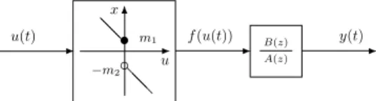
Fig. 1. The input nonlinear system with the preload nonlinearity.
use the dual-rate data, and then propose a multi-innovation SG algorithm to estimate the unknown parameters of a class of
input nonlinear systems.
Briefly, the letter is organized as follows. Section
2
describes the problem formulation of the dual-rate systems with
preload nonlinearity and derives a suitable model. Section
3
discusses an SG algorithm and a multi-innovation stochastic
gradient algorithm for the obtained dual-rate model. Section
4
provides an illustrative example. Finally, concluding remarks
are given in Section
5
.
2. Problem description
Consider the following dual-rate nonlinear system, shown in
Fig. 1
:
A
(
z
)
y
(
t
)
=
B
(
z
)
f
(
u
(
t
)),
(1)
A
(
z
)
:=
1
+
a
1z
−1+
a
2z
−2+ · · · +
a
nz
−n,
B
(
z
)
:=
b
1z
−1+
b
2z
−2+
b
3z
−3+ · · · +
b
nz
−n,
where
y
(
t
)
is the system output,
u
(
t
)
is the system input, and
z
−1is a unit backward shift operator:
z
−1y
(
t
)
=
y
(
t
−
1
)
, the
function
f
(
u
(
t
))
is a preload nonlinearity and can be expressed as
f
(
u
(
t
))
=
−
u
(
t
)
+
m
1,
u
(
t
)
>
0
,
−
u
(
t
)
−
m
2,
u
(
t
) <
0
.
The numbers
m
1and
−
m
2are two preload points.
The dual-rate sampled-data system under consideration in this letter assumes that all input data
{
u
(
t
),
t
=
0
,
1
,
2
, . . .
}
are available and so are only the scarce output data
y
(
qt
),
q
>
2
,
t
=
0
,
1
,
2
, . . .
. The intersample outputs or missing
outputs
y
(
qt
+
j
),
j
=
1
,
2
, . . . ,
q
−
1 are unavailable. The following uses the polynomial transformation technique to
generate a new dual-rate model which works on the dual-rate sampled-data [
19
]. Let
A
(
z
)
=
(
1
−
z
1z
−1)(
1
−
z
2z
−1)
· · ·
(
1
−
z
nz
−1),
where
z
i,i
=
1
,
2
, . . . ,
n
, are the roots of
A
(
z
)
[
15
]. Define the polynomials,
r
(
z
)
:=
n
i=1(
1
+
z
iz
−1+
z
i2z
−2+ · · · +
z
q−1 iz
−q+1)
=
1
+
r
1z
−1+
r
2z
−2+ · · · +
r
mz
−m,
m
:=
n
(
q
−
1
),
α(
z
)
:=
r
(
z
)
A
(
z
)
=
1
+
α
1z
−q+
α
2z
−2q+ · · · +
αn
z
−nq,
(2)
β(
z
)
:=
r
(
z
)
B
(
z
)
=
β
1z
−1+
β
2z
−2+ · · · +
βnq
z
−nq.
(3)
Multiplying both sides of
(1)
by
r
(
z
)
yields
α(
z
)
y
(
t
)
=
β(
z
)
f
(
u
(
t
))
. Consider a disturbance in a physical system, introducing
a noise term
v(
t
)
gives
α(
z
)
y
(
t
)
=
β(
z
)
f
(
u
(
t
))
+
v(
t
).
(4)
For simplification, we introduce two switching functions:
h
1[
u
(
t
)
] =
1
,
if
u
(
t
)
>
0
,
0
,
if
u
(
t
) <
0
,
h
2[
u
(
t
)
] =
0
,
if
u
(
t
)
>
0
,
−
1
,
if
u
(
t
) <
0
.
Then the preload nonlinearity
f
(
u
(
t
))
can be written as
f
(
u
(
t
))
= −
u
(
t
)
+
m
1h
1(
u
(
t
))
+
m
2h
2(
u
(
t
)),
(5)
and Eq.
(4)
can be written as
β
1m
2, β
2m
2, β
3m
2, . . . , βnq
m
2, α
1, α
2, α
3, . . . , αn
]
T∈
R
3nq+n,
ϕ
(
t
)
:= [−
u
(
t
−
1
),
−
u
(
t
−
2
),
−
u
(
t
−
3
), . . . ,
−
u
(
t
−
nq
),
h
1(
u
(
t
−
1
)),
h
1(
u
(
t
−
2
)),
h
1(
u
(
t
−
3
)), . . . ,
h
1(
u
(
t
−
nq
)),
h
2(
u
(
t
−
1
)),
h
2(
u
(
t
−
2
)),
h
2(
u
(
t
−
3
)), . . . ,
h
2(
u
(
t
−
nq
)),
−
y
(
t
−
q
),
−
y
(
t
−
2
q
), . . . ,
−
y
(
t
−
nq
)
]
T∈
R
3nq+n.
From
(6)
, we have the identification model,
y
(
t
)
=
ϕ
T(
t
)
θ
+
v(
t
)
or
y
(
qt
)
=
ϕ
T(
qt
)
θ
+
v(
qt
).
(7)
The vector
ϕ
(
qt
)
contains only the available measurement outputs and inputs.
Let
θ
ˆ
(
qt
)
be the estimate of
θ
at time
qt
. The following SG algorithm can estimate the parameter vector
θ
in
(7)
[
15
,
19
]:
ˆ
θ
(
qt
)
= ˆ
θ
(
qt
−
q
)
+
ϕ
(
qt
)
r
(
qt
)
e
(
qt
),
(8)
ˆ
θ
(
qt
+
i
)
= ˆ
θ
(
qt
),
i
=
0
,
1
,
2
, . . . ,
q
−
1
,
(9)
e
(
qt
)
=
y
(
qt
)
−
ϕ
T(
qt
)
θ
ˆ
(
qt
−
q
),
(10)
r
(
qt
)
=
r
(
qt
−
q
)
+ ∥
ϕ
(
qt
)
∥
2,
r
(
0
)
=
1
,
(11)
where 1
/
r
(
qt
)
is the step-size and the norm of matrix
X
is defined by
∥
X
∥
2:=
tr
[
XX
T]
.
In order to enhance the convergence rate of the SG algorithm, we extend the SG algorithm such that the parameter
estimation accuracy can be improved. Such an algorithm is derived from the multi-innovation identification theory [
32
]. At
time
qt
, the SG algorithm only uses the current data
y
(
qt
)
and
ϕ
(
qt
)
thus has slow convergence rate. Referring to [
32
], we
derive a new algorithm by expanding the single innovation
e
(
qt
)
to an innovation vector:
E
(
p
,
qt
)
= [
e
(
qt
),
e
(
qt
−
q
),
e
(
qt
−
2
q
), . . . ,
e
(
qt
−
(
p
−
1
)
q
)
]
T≈ [
y
(
qt
)
− ˆ
θ
T(
qt
−
q
)
ϕ
(
qt
),
y
(
qt
−
q
)
− ˆ
θ
T(
qt
−
q
)
ϕ
(
qt
−
q
), . . . ,
y
(
qt
−
(
p
−
1
)
q
)
− ˆ
θ
T(
qt
−
q
)
ϕ
(
qt
−
(
p
−
1
)
q
)
]
T∈
R
p,
which uses the past data
{
y
(
qt
−
iq
),
ϕ
ˆ
(
qt
−
iq
)
:
i
=
1
,
2
, . . . ,
p
−
1
}
, where
p
represents the innovation length.
Define the information matrix
Φ
(
p
,
qt
)
and the stacked output vector
Y
(
p
,
qt
)
as
Φ
(
p
,
qt
)
:= [
ϕ
(
qt
),
ϕ
(
qt
−
q
),
ϕ
(
qt
−
2
q
), . . . ,
ϕ
(
qt
−
(
p
−
1
)
q
)
]
T∈
R
p×(3nq+n),
Y
(
p
,
qt
)
:= [
y
(
qt
),
y
(
qt
−
q
),
y
(
qt
−
2
q
), . . . ,
y
(
qt
−
(
p
−
1
)
q
)
]
T∈
R
p.
The innovation vector
E
(
p
,
qt
)
can be expressed as
E
(
p
,
qt
)
=
Y
(
p
,
qt
)
−
Φ
(
p
,
qt
)
θ
ˆ
(
qt
−
q
).
Referring to the multi-innovation stochastic gradient method for linear regression models [
32–41
], we can obtain the
following multi-innovation stochastic gradient (MISG) algorithm for the input nonlinear system:
ˆ
θ
(
qt
)
= ˆ
θ
(
qt
−
q
)
+
Φ
T(
p
,
qt
)
r
(
qt
)
E
(
p
,
qt
),
(12)
ˆ
θ
(
qt
+
i
)
= ˆ
θ
(
qt
),
i
=
0
,
1
,
2
, . . . ,
q
−
1
,
(13)
E
(
p
,
qt
)
=
Y
(
p
,
qt
)
−
Φ
(
p
,
qt
)
θ
ˆ
(
qt
−
q
),
(14)
Y
(
p
,
qt
)
= [
y
(
t
),
y
(
qt
−
q
),
y
(
qt
−
2
q
), . . . ,
y
(
qt
−
(
p
−
1
)
q
)
]
T,
(15)
Φ
(
p
,
qt
)
= [
ϕ
(
qt
),
ϕ
(
qt
−
q
),
ϕ
(
qt
−
2
q
), . . . ,
ϕ
(
qt
−
(
p
−
1
)
q
)
]
T,
(16)
ϕ
(
qt
)
= [−
u
(
qt
−
1
),
−
u
(
qt
−
2
),
−
u
(
qt
−
3
), . . . ,
−
u
(
qt
−
nq
),
h
1(
u
(
qt
−
1
)),
h
1(
u
(
qt
−
2
)),
h
1(
u
(
qt
−
3
)), . . . ,
h
1(
u
(
qt
−
nq
)),
h
2(
u
(
qt
−
1
)),
h
2(
u
(
qt
−
2
)),
h
2(
u
(
qt
−
3
)), . . . ,
h
2(
u
(
qt
−
nq
)),
−
y
(
qt
−
q
),
−
y
(
qt
−
2
q
), . . . ,
−
y
(
qt
−
nq
)
]
T,
(17)
r
(
qt
)
=
r
(
qt
−
q
)
+ ∥
ϕ
(
qt
)
∥
2,
r
(
0
)
=
1
.
(18)
Because
E
(
p
,
qt
)
∈
R
pis an innovation vector, namely, the multi-innovation, the algorithm in
(12)–(18)
is called the
Table 1
The SG estimates and errors.
t 100 200 300 500 1000 1500 2000 2500 3000 True values
α
1 0.26952 0.28334 0.29128 0.30112 0.31416 0.32162 0.32683 0.33082 0.33406 0.95000α
2−
0.00894−
0.00198 0.00176 0.00619 0.01180 0.01490 0.01703 0.01864 0.01994 0.36000β
1 0.45187 0.44961 0.44820 0.44635 0.44378 0.44225 0.44117 0.44033 0.43964 0.40000β
2 0.04488 0.04499 0.04512 0.04535 0.04574 0.04599 0.04619 0.04635 0.04648 0.10000β
3−0.12242
−0.11634
−0.11287
−0.10859
−0.10297
−0.09978
−0.09756
−0.09587
−0.09450
0.09000β
4 0.17240 0.17265 0.17272 0.17274 0.17268 0.17262 0.17257 0.17253 0.17250 0.18000β
1m1 0.10862 0.11389 0.11696 0.12079 0.12590 0.12884 0.13090 0.13248 0.13376 0.08000β
2m1 0.08160 0.08274 0.08340 0.08421 0.08527 0.08586 0.08627 0.08657 0.08681 0.02000β
3m1−0.05231
−0.05641
−0.05855
−0.06101
−0.06398
−0.06555
−0.06659
−0.06736
−0.06797
0.01800β
4m1 0.03158 0.03275 0.03346 0.03436 0.03557 0.03625 0.03673 0.03709 0.03738 0.03600β
1m2 0.10997 0.11638 0.11990 0.12413 0.12956 0.13259 0.13468 0.13627 0.13755 0.04000β
2m2 0.08296 0.08523 0.08634 0.08755 0.08893 0.08961 0.09005 0.09036 0.09060 0.01000β
3m2−0.05095
−0.05392
−0.05561
−0.05767
−0.06033
−0.06181
−0.06281
−0.06358
−0.06418
0.00900β
4m2 0.03293 0.03524 0.03640 0.03770 0.03922 0.04000 0.04051 0.04088 0.04117 0.01800δ
(%) 73.32206 72.01943 71.28427 70.38527 69.21194 68.54941 68.08961 67.73869 67.45562 Table 2The MISG estimates and errors withp
=
10.t 100 200 300 500 1000 1500 2000 2500 3000 True values
α
1 0.92857 0.93510 0.93788 0.94061 0.94330 0.94447 0.94516 0.94564 0.94599 0.95000α
2 0.34751 0.35133 0.35296 0.35455 0.35611 0.35680 0.35720 0.35748 0.35768 0.36000β
1 0.40053 0.40038 0.40031 0.40024 0.40017 0.40013 0.40012 0.40010 0.40009 0.40000β
2 0.10148 0.10115 0.10098 0.10080 0.10060 0.10051 0.10045 0.10041 0.10038 0.10000β
3 0.07593 0.07963 0.08130 0.08301 0.08477 0.08558 0.08607 0.08641 0.08667 0.09000β
4 0.17865 0.17903 0.17918 0.17933 0.17948 0.17954 0.17958 0.17961 0.17963 0.18000β
1m1 0.06549 0.06661 0.06713 0.06765 0.06820 0.06844 0.06859 0.06870 0.06877 0.08000β
2m1 0.01912 0.02051 0.02116 0.02184 0.02257 0.02290 0.02311 0.02325 0.02335 0.02000β
3m1 0.04511 0.04063 0.03840 0.03595 0.03322 0.03189 0.03104 0.03045 0.02999 0.01800β
4m1 0.03443 0.03538 0.03578 0.03616 0.03652 0.03665 0.03673 0.03677 0.03681 0.03600β
1m2 0.04564 0.04679 0.04733 0.04790 0.04850 0.04877 0.04894 0.04906 0.04915 0.04000β
2m2−0.00038
0.00104 0.00172 0.00244 0.00322 0.00358 0.00381 0.00397 0.00408 0.01000β
3m2 0.02514 0.02070 0.01849 0.01609 0.01340 0.01210 0.01128 0.01070 0.01026 0.00900β
4m2 0.01475 0.01573 0.01616 0.01658 0.01699 0.01716 0.01725 0.01731 0.01736 0.01800δ
(%) 4.16769 3.30340 2.92591 2.55473 2.19616 2.04601 1.96042 1.90417 1.863954. Example
Consider the following system,
A
(
z
−1)
y
(
t
)
=
B
(
z
−1)
f
(
u
(
t
))
+
v(
t
),
A
(
z
−1)
=
1
+
a
1z
−1+
a
2z
−2=
1
+
0
.
5
z
−1+
0
.
6
z
−2,
B
(
z
−1)
=
b
1z
−1+
b
2z
−2=
0
.
4
z
−1+
0
.
3
z
−2,
f
(
u
(
t
))
= −
u
(
t
)
+
0
.
2
h
1(
u
(
t
))
+
0
.
1
h
2(
u
(
t
)),
in simulation,
{
u
(
t
)
}
is taken as a persistently excited signal sequence with zero mean and unit variance, and
{
v(
t
)
}
as a
white noise sequence with zero mean and variance
σ
2=
0
.
10
2. Taking
q
=
2 and
r
(
z
)
=
1
−
0
.
5
z
−1+
0
.
6
z
−2, we have
α(
z
)
=
r
(
z
)
A
(
z
)
=
1
+
0
.
95
z
−2+
0
.
36
z
−4,
β(
z
)
=
r
(
z
)
B
(
z
)
=
0
.
4
z
−1+
0
.
1
z
−2+
0
.
09
z
−3+
0
.
18
z
−4,
θ
= [
β
1, β
2, β
3, β
4, β
1m
1, β
2m
1, β
3m
1, β
4m
1, β
1m
2, β
2m
2, β
3m
2, β
4m
2, α
1, α
2]
T= [
0
.
4
,
0
.
1
,
0
.
09
,
0
.
18
,
0
.
08
,
0
.
02
,
0
.
018
,
0
.
036
,
0
.
04
,
0
.
01
,
0
.
009
,
0
.
018
,
0
.
95
,
0
.
36
]
T.
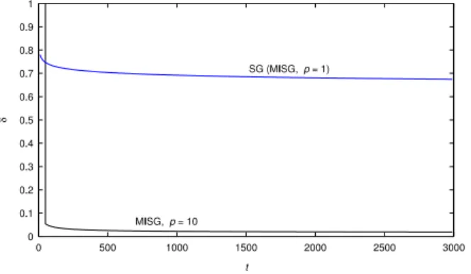
Applying the SG algorithm and the MISG algorithm to estimate the parameters of this system, the parameter estimates and
their errors are shown in
Tables 1
–
2
and the parameter estimation errors
δ
:= ∥ˆ
θ
−
θ
∥
/
∥
θ
∥
versus
t
are shown in
Fig. 2
.
From
Tables 1
–
2
and
Fig. 2
, we can see that the convergence rate of the MISG algorithm is faster than the SG algorithm
and the parameter estimates given by the MISG algorithm converge their true values with the increasing of
t
.
5. Conclusions
This letter uses the polynomial transformation technique to study identification problems for a class of dual-rate input
nonlinear systems and presents a multi-innovation stochastic gradient algorithm by expanding the scalar innovations to the
Fig. 2. The parameter estimation errors
δ
versust.innovation vector. The convergence of the proposed algorithm can be analyzed in a similar method in [
32
]. The proposed
method can be extended to other nonlinear systems, e.g., non-uniformly sampled-data nonlinear systems [
42–48
].
References
[1] M. Dehghan, M. Hajarian, Two algorithms for finding the Hermitian reflexive and skew-Hermitian solutions of Sylvester matrix equations, Applied Mathematics Letters 24 (4) (2011) 444–449.
[2] H.R. Xu, Z. Sun, S.L. Xie, An iterative algorithm for solving a kind of discrete HJB equation withM-functions, Applied Mathematics Letters 24 (3) (2011) 279–282.
[3] F. Ding, P.X. Liu, G. Liu, Gradient based and least-squares based iterative identification methods for OE and OEMA systems, Digital Signal Processing 20 (3) (2010) 664–677.
[4] Y.J. Liu, D.Q. Wang, et al., Least-squares based iterative algorithms for identifying Box–Jenkins models with finite measurement data, Digital Signal Processing 20 (5) (2010) 1458–1467.
[5] D.Q. Wang, G.W. Yang, R.F. Ding, Gradient-based iterative parameter estimation for Box–Jenkins systems, Computers & Mathematics with Applications 60 (5) (2010) 1200–1208.
[6] F. Ding, Y.J. Liu, B. Bao, Gradient based and least squares based iterative estimation algorithms for multi-input multi-output systems, Proceedings of the Institution of Mechanical Engineers, Part I: Journal of Systems and Control Engineering 226 (1) (2012) 43–55.
[7] F. Ding, J. Ding, Least squares parameter estimation with irregularly missing data, International Journal of Adaptive Control and Signal Processing 24 (7) (2010) 540–553.
[8] J. Ding, F. Ding, X.P. Liu, G. Liu, Hierarchical least squares identification for linear SISO systems with dual-rate sampled-data, IEEE Transactions on Automatic Control 56 (11) (2011) 2677–2683.
[9] J. Ding, F. Ding, Bias compensation based parameter estimation for output error moving average systems, International Journal of Adaptive Control and Signal Processing 25 (12) (2011) 1100–1111.
[10] F. Ding, Y. Shi, T. Chen, Auxiliary model based least-squares identification methods for Hammerstein output-error systems, Systems & Control Letters 56 (5) (2007) 373–380.
[11] D.Q. Wang, Y.Y. Chu, et al., Auxiliary model-based RELS and MI-ELS algorithms for Hammerstein OEMA systems, Computers & Mathematics with Applications 59 (9) (2010) 3092–3098.
[12] Y.J. Liu, J. Sheng, R.F. Ding, Convergence of stochastic gradient estimation algorithm for multivariable ARX-like systems, Computers & Mathematics with Applications 59 (8) (2010) 2615–2627.
[13] F. Ding, G. Liu, X.P. Liu, Partially coupled stochastic gradient identification methods for non-uniformly sampled systems, IEEE Transactions on Automatic Control 55 (8) (2010) 1976–1981.
[14] J. Ding, Y. Shi, et al., A modified stochastic gradient based parameter estimation algorithm for dual-rate sampled-data systems, Digital Signal Processing 20 (4) (2010) 1238–1247.
[15] J. Chen, L.X. Lv, R.F. Ding, Parameter estimation for dual-rate sampled data systems with preload nonlinearities, Advances in Intelligent and Soft Computing 125 (2011) 43–50.
[16] F. Ding, T. Chen, Parameter estimation of dual-rate stochastic systems by using an output error method, IEEE Transactions on Automatic Control 50 (9) (2005) 1436–1441.
[17] S.C. kadu, M. Bhushan, R.D. Gudi, Optimal sensor network design for multirate systems, Journal of Process Control 18 (6) (2008) 594–609. [18] J. Ding, L.L. Han, X.M. Chen, Time series AR modeling with missing observations based on the polynomial transformation, Mathematical and Computer
Modelling 51 (5–6) (2010) 527–536.
[19] F. Ding, P.X. Liu, H.Z. Yang, Parameter identification and intersample output estimation for dual-rate systems, IEEE Transactions on Systems, Man, and Cybernetics, Part A: Systems and Humans 38 (4) (2008) 966–975.
[20] F. Ding, P.X. Liu, Y. Shi, Convergence analysis of estimation algorithms of dual-rate stochastic systems, Applied Mathematics and Computation 176 (1) (2006) 245–261.
[21] F. Ding, T. Chen, Combined parameter and output estimation of dual-rate systems using an auxiliary model, Automatica 40 (10) (2004) 1739–1748. [22] Y. Shi, F. Ding, T. Chen, 2-norm based recursive design of transmultiplexers with designable filter length, Circuits, Systems, and Signal Processing 25
(4) (2006) 447–462.
[23] B. Yu, Y. Shi, H.N. Huang,l2
−
l∞filtering for multirate systems using lifted models, Circuits, Systems, and Signal Processing 27 (5) (2008) 699–711. [24] Y. Shi, T. Chen, Optimal design of multi-channel transmultiplexers with stopband energy and passband magnitude constraints, IEEE Transactions onCircuits and Systems II: Analog and Digital Signal Processing 50 (9) (2003) 659–662.
[25] J. Chen, Y. Zhang, R.F. Ding, Auxiliary model based multi-innovation algorithms for multivariable nonlinear systems, Mathematical and Computer Modelling 52 (9–10) (2010) 1428–1434.
[26] J. Chen, X.P. Wang, R.F. Ding, Gradient based estimation algorithm for Hammerstein systems with saturation and dead-zone nonlinearities, Applied Mathematical Modelling 36 (1) (2012) 238–243.
[27] B. Yu, H. Fang, Y. Shi, Identification of Hammerstein output-error systems with two-segment nonlinearities: algorithm and applications, Control and Intelligent Systems 38 (4) (2010) 194–201.
[28] E.W. Bai, Identification of linear systems with hard input nonlinearities of known structure, Automatica 38 (5) (2002) 853–860.
[29] J. Vörös, Modeling and parameter identification of systems with multi-segment piecewise-linear characteristics, IEEE Transactions on Automatic Control 47 (1) (2002) 184–188.
[30] J. Vörös, Modeling and identification of systems with backlash, Automatica 46 (2) (2010) 369–374.
[31] F. Ding, X.P. Liu, G. Liu, Identification methods for Hammerstein nonlinear systems, Digital Signal Processing 21 (2) (2011) 215–238. [32] F. Ding, T. Chen, Performance analysis of multi-innovation gradient type identification methods, Automatica 43 (1) (2007) 1–14.
[33] F. Ding, P.X. Liu, G. Liu, Auxiliary model based multi-innovation extended stochastic gradient parameter estimation with colored measurement noises, Signal Processing 89 (10) (2009) 1883–1890.
[34] L.L. Han, F. Ding, Multi-innovation stochastic gradient algorithms for multi-input multi-output systems, Digital Signal Processing 19 (4) (2009) 545–554.
[35] Y.J. Liu, Y.S. Xiao, X.L. Zhao, Multi-innovation stochastic gradient algorithm for multiple-input single-output systems using the auxiliary model, Applied Mathematics and Computation 215 (4) (2009) 1477–1483.
[36] J.B. Zhang, F. Ding, Y. Shi, Self-tuning control based on multi-innovation stochastic gradient parameter estimation, Systems & Control Letters 58 (1) (2009) 69–75.
[37] F. Ding, Several multi-innovation identification methods, Digital Signal Processing 20 (4) (2010) 1027–1039.
[38] Y.J. Liu, L. Yu, et al., Multi-innovation extended stochastic gradient algorithm and its performance analysis, Circuits, Systems, and Signal Processing 29 (4) (2010) 649–667.
[39] D.Q. Wang, F. Ding, Performance analysis of the auxiliary models based multi-innovation stochastic gradient estimation algorithm for output error systems, Digital Signal Processing 20 (3) (2010) 750–762.
[40] F. Ding, P.X. Liu, G. Liu, Multi-innovation least squares identification for linear and pseudo-linear regression models, IEEE Transactions on Systems, Man, and Cybernetics, Part B: Cybernetics 40 (3) (2010) 767–778.
[41] F. Ding, G. Liu, X.P. Liu, Parameter estimation with scarce measurements, Automatica 47 (8) (2011) 1646–1655.
[42] D.Q. Wang, F. Ding, Extended stochastic gradient identification algorithms for Hammerstein–Wiener ARMAX systems, Computers & Mathematics with Applications 56 (12) (2008) 3157–3164.
[43] D.Q. Wang, F. Ding, Least squares based and gradient based iterative identification for Wiener nonlinear systems, Signal Processing 91 (5) (2011) 1182–1189.
[44] F. Ding, L. Qiu, T. Chen, Reconstruction of continuous-time systems from their non-uniformly sampled discrete-time systems, Automatica 45 (2) (2009) 324–332.
[45] F. Ding, T. Chen, Identification of Hammerstein nonlinear ARMAX systems, Automatica 41 (9) (2005) 1479–1489.
[46] Y.J. Liu, L. Xie, et al., An auxiliary model based recursive least squares parameter estimation algorithm for non-uniformly sampled multirate systems, Proceedings of the Institution of Mechanical Engineers, Part I: Journal of Systems and Control Engineering 223 (4) (2009) 445–454.
[47] L. Xie, H.Z. Yang, et al., Modeling and identification for non-uniformly periodically sampled-data systems, IET Control Theory and Applications 4 (5) (2010) 784–794.