Li C, Zhu S, Xu YL and Xiao Y (2013) 2.5D large eddy simulation of vertical axis wind turbine in consideration of high angle of attack flow. Renewable Energy. 51: 317-330.
2.5D Large Eddy Simulation of Vertical Axis Wind Turbine
in High Angle of Attack Flow
Chao Li1,2, Songye Zhu1,*, You-lin Xu1 and Yiqing Xiao2
1. Department of Civil and Structural Engineering, The Hong Kong Polytechnic University, Hung Hom, Kowloon, Hong Kong SAR, China
2. Shenzhen Graduate School, Harbin Institute of Technology, Shenzhen 518055, China
* Correspondence author: Dr. S. Zhu, Email: [email protected], Tel: (+852) 3400 3964, Fax: (+852) 2334 6389
Abstract
A renewed interest in vertical axis wind turbines (VAWTs) has been seen recently. Computational fluid dynamics (CFD) is regarded as a promising technique for aerodynamic studies of VAWTs. In particular, 2D unsteady Reynolds-averaged Navier-Stokes (URANS) is commonly adopted, although past studies on VAWTs revealed the limited accuracy of 2D URANS. This paper investigated the feasibility and accuracy of three different CFD approaches, namely 2D URANS, 2.5D URANS and 2.5D Large Eddy Simulations (LES), in the aerodynamic characterization of straight-bladed VAWT (SBVAWT), with a focus on the capability of the 2.5D LES approach in CFD simulation of high angle of attack (AOA) flow. The 2.5D model differs from a full 3D model in that only a certain length of blades is modeled with periodic boundaries at the two extremities of the domain. The applications of these three approaches were systematically examined in the aerodynamic simulations of a single static airfoil and a 3-blade SBVAWT at different rotating speeds. Their capabilities to predict the aerodynamic forces were evaluated through a comparison with the wind tunnel results obtained by other researchers, with particular attention to high AOA flow beyond stall. Among the three methods, 2.5D LES yielded the best agreement with the experimental results in both cases. Detailed examinations of simulated flow field revealed that 2.5D LES produces more realistic 3D vortex diffusion after flow separation, resulting in more accurate predictions of aerodynamic coefficients in static or dynamic stall situations. It is noteworthy that 2.5D LES cannot capture the effect of tip vortex and vertical flow divergence in VAWTs, which used to be regarded by some researchers as the major cause of overprediction of VAWT power in 2D URANS. In this study, the considerably improved results achieved by 2.5D LES imply that the poor accuracy of URANS method is mainly due to its inherent limitation in vortex modeling. In general, 2.5D LES showed good agreement with experimental results at a relatively low tip speed ratio (TSR), but only fair agreement at a high TSR. Compared with the other two approaches, 2.5D LES is regarded as a more promising and effective CFD tool for investigating the aerodynamic characteristics of VAWTs, particularly their self-starting features corresponding to very low rotation speeds.
Keywords: 2.5D large eddy simulation; High angle of attack; Straight-bladed vertical axis wind turbine; Computational fluid dynamics;
1
Introduction
The depletion of fossil energy resources and global warming trends has led to the recognition of a low carbon economy as an international strategy for sustainable development. Among several green and renewable energy sources, wind energy has seen a rapid growth worldwide and will play an increasingly important role in the future economy. Wind turbines are typical devices that convert the kinetic energy of wind into electricity. Although horizontal axis wind turbines (HAWTs) are the mainstream of commercial wind turbines at present, we have seen a renewed interest in vertical axis wind turbines (VAWTs) recently. Compared with a common HAWT, a VAWT offers several advantages [1, 2]: (1) a VAWT is omni-directional and thus insensitive to wind directions; (2) VAWT’s blades live longer because they are under constant gravity and inertia force in terms of quantity and direction; (3) a VAWT is less sensitive to cross wind and turbulence, so that a small-scale VAWT can be mounted close to the ground, on a rooftop or in an urban area where wind is more turbulent than in an open wind farm; and (4) aVAWT is typically slower and quieter than a HAWT, and thus causes less noise problems.
Research and development of VAWTs are relatively limited in comparison with those on HAWTs. For example, more research and development of VAWTs are required for higher power efficiencies, better self-starting features, and longer service life. Some efforts were made to optimize the characteristics of the airfoil blades in VAWTs, including airfoil section, thickness and camber, solidity, and pitch angle [3-5]. Different blade configurations, such as straight,
troposkein curved and helical twisted blade shapes, have been examined as well [6-9].
Investigations on VAWTs require a deep insight into their complex aerodynamics, such as dynamic stall and 3D flow vortices. Wind tunnel tests are a widely accepted means to study the aero- and structural dynamics. The aerodynamic forces on rotor blades are often measured by pressure taps mounted on the blade surface or strain gauges on the arms of the turbine [10-12].
Limited by the present measurement instruments or methodology, however, the wind tunnel results are often too simple and cannot provide a comprehensive picture of the complex aerodynamic behavior of VAWTs. Furthermore, the tests and measurements are complex and costly, and the post-processing of the data is often necessary to improve the quality of the measurement data.
Computational fluid dynamics (CFD), as a promising technique in wind engineering research, has attracted growing interest in the past two decades. Compared with the conventional experimental approaches, CFD could provide more details about flow field without any need for complicated control and measurement systems. It also provides an inexpensive solution to performing systematic analyses, such as the parametric studies required for performance optimization of VAWTs. Subject to the constraint of computational resources and time, most researchers adopted 2D unsteady Reynolds-Averaged Navier–Stokes (URANS) simulations in the performance study of VAWTs. However, compared with wind tunnel tests, 2D URANS simulations tend to overestimate the power coefficients, although they can approximately replicate the variation trend of experimental power coefficients [11, 13-15]. Some researchers attributed this discrepancy to the effects of the tip loss or flow divergence in real VAWTs, both of which are not reflected in 2D URANS simulations. The former refers to the aerodynamic
force change caused by the presence of vortices at the blade tips, whereas the latter refers to the effective blockage that restricts flow divergence above and below the swept area of the finite-span turbine. For example, Howell et al. [13] adopted the renormalization group (RNG)
ε
−
k turbulence model and found that the 3D simulations agreed with experimental data better than the 2D simulations. They concluded that 2D simulation is unable to capture the effects of the tip vortices in the real turbine. Mukinovi et al. [14] also found considerably a higher peak torque in 2D shear stress transport (SST) k−ω simulations than that in 3D results, and attributed the difference to the influence of finite span and drag of the traverse in the 3D model.
McLaren [11] proposed the use of effective upstream velocity and effective blade height to adjust 2D URANS simulated tangential forces in order to match the experimental results. These studies demonstrated the shortcoming of 2D URANS simulations due to neglecting the effects of blade tip vortices or flow divergence, and implied that an accurate simulation of VAWT flow could be achieved if the finite span of blades can be properly modeled in the full-scale sophisticated 3D modeling of a VAWT. However, some critical factors, such as the blade aerodynamics in stall flow at a high angle of attack (AOA) and the capability of various CFD turbulence models, have been overlooked in the past, although it is well recognized that they may have a profound impact on the simulation of power efficiency and overall aerodynamics of VAWTs.
Unlike the airfoil blades in an aircraft, VAWT blades frequently experience high AOA beyond the stall angle, especially when they operates at a low tip speed ratio (TSR) (λ<4) [16]. Figure 1 shows the plan view of a 3-blade straight-bladed VAWT (SBVAWT). The oncoming flow velocity seen by each blade is the vectorial addition of the rotating speed Ωr and the incoming wind speed u∞. Thus, the resultant velocity experiences variations in magnitude ur and AOA
α, both of which depend on the azimuthal position θ of the blade and the TSR λ. The TSR is defined as the ratio of the rotating speed Ωr to the wind speed u∞. When the blade is at an
upwind azimuthal position (i.e., 0°≤θ ≤180°), the velocity ur and AOA α can be
approximated by:
(
2)
0.5 sin 2 1+ λ θ +λ =u∞ ur (1) ⎟ ⎠ ⎞ ⎜ ⎝ ⎛ + = − λ θ θ α sin cos tan 1 (2)In the downwind zone (i.e. 180°<θ <360°), the airfoil located in the shedding wake from upwind zone sees a disturbed flow that makes the determination of AOA more complex. Figure 2 shows the variation of AOA α with the azimuthal angle θ (0°≤θ ≤180°) for different TSRs based on the estimation by Equation (2). The stall occurs at a relatively high AOA. In general, the static stall angles of symmetric VAWT airfoils range from 10° to 15° [17]. As illustrated in Figure 2, the stall of the airfoil always takes place whenλ<4. Such a TSR is common in small VAWTs. Particularly at a very low TSR that often occurs in the starting process, the maximum AOA is far beyond the stall angle. Therefore, good reproduction of high AOA flow is inevitable in assessing VAWT performance.
The airfoil flow at high AOA is three dimensional, highly separated and unsteady with a nonlinear lift variation [18]. Cummings et al. [19] pointed out several important issues for the
accurate simulation of high AOA flow fields, such as turbulence modeling and domain
aerodynamic simulations of VAWTs. For example, the URANS models widely used in VAWT simulations often fail to provide accurate results for high AOA flows where there is large-scale turbulence in separated flows. On the other hand, Detached Eddy Simulation (DES) or Large Eddy Simulation (LES), although recognized as more advanced and powerful turbulence models, are rarely found in the past CFD studies of VAWTs. Secondly, the certain potential limitation in 2D CFD simulation is prone to be overlooked; for example, the flow diversities in spanwise direction of blades cannot be considered in 2D CFD simulations. Sørensen and Michelsen [20]
found that 2D Navier-Stokes solvers overpredict the lift and drag of the stalled airfoil, even when AOA was only slightly above the stall angle. Quasi-3D or full 3D simulation should be adopted to overcome the shortcoming of the conventional 2D model. In Quasi-3D CFD simulation approach, the 2D model is extended in a spanwise direction for a considerable length in order to achieve a realistic reproduction of 3D separated vortices. The spanwise length is not fully modeled in such a 3D simulation, so that it is referred to as 2.5D CFD simulation hereinafter in order to differentiate it from the conventional 2D and 3D simulations. Gao et al. [21] performed 2.5D LES simulations of the flow field around a single static airfoil and found that the 2D model is not adequate for predicting unsteady flow structures with large-scale separations around airfoils at relatively high AOAs. Furthermore, Travin et al. [22], Bertagnolio et al. [23], and IM and Zha [24] presented simulations of a single airfoil beyond stall using the DES method, which is essentially a hybrid model of RANS and LES. Results of the 2.5 DES model are clearly superior over those of the 2.5D URANS models.
Although a sophisticated full 3D CFD simulation is always desirable in consideration of the aforementioned reasons, its extremely high computational cost prevents its wide applications by researchers or designers at present. An efficient, convenient and high-fidelity CFD simulation strategy for VAWTs is still being sought. In view of this, a systematic CFD study was performed to investigate the feasibility and accuracy of 2D URANS, 2.5D URANS and 2.5D LES in predicting the aerodynamic characteristics of a single static airfoil blade and a SBVAWT. First, the flow field of a single static airfoil was simulated using the three different methods with a focus on the stall flow at high AOA. The comparisons with wind tunnel tests clearly indicated 2.5D LES resulted in minimal discrepancies in lift and drag coefficients for a wide range of AOA. Compared with 2D URANS, 2.5D URANS provided considerably improved results, although its simulation accuracy was still limited at high AOA. Second, the flow field of a 3-blade SBVAWT was simulated at different rotating speeds. Again, 2.5D LES provided the best agreement with experimental results and the most realistic description of aerodynamic details among the three methods, especially at the low rotating speed. Unlike the simulation of the single static airfoil, only small discrepancies in the simulated blade forces were discovered between 2D and 2.5D URANS methods. This finding implies that the VAWT flow is characterized by the dynamic stall of the rotating blade which has negligible diversities in the spanwise direction and is quite different from static stall flow. Moreover, URANS, either 2D or 2.5D, could not properly predict the leading edge separation in dynamic stall.
2
2.5D LES of Single Airfoil Blade
The CFD simulation of airfoil flow with an AOA higher than 45° is rarely discussed in the literature. However, blades encounter a very high AOA as they rotate at a low TSR (as shown in
Figure 2). The aerodynamic data of static airfoil at AOAs ranging from 0° to 360° (0° to 180° for symmetry airfoil) is the fundamental input of a double-multiple streamtube (DMS) model that is a widely accepted method for evaluating the power of VAWTs in engineering practice [1]. In this section, the capabilities of 2D URANS, 2.5D URANS, and 2.5D LES in the simulation of a single static airfoil NACA0018 at a full range of AOAs were examined and compared, with focus on the efficacy of different CFD simulation strategies.
2.1 CFD Simulation of Single Static Airfoil
Airfoil NACA0018 is one of the commonly used blade sections in VAWTs. Delft University of Technology conducted wind tunnel tests of NACA0018 airfoil and obtained good-quality aerodynamic data for a full range of AOAs [4, 25]. These experimental data offered a good opportunity to examine the capability of various CFD strategies at very high AOAs. The commercial CFD software Fluent was employed in flow computation. Fluent is based on the finite volume method (FVM) which discretizes the computational domain into some small volumes and has been verified in many applications. The detailed computational treatments and algorithms are explained as follows.
2.1.1 Mesh geometry and boundary conditions
Figure 3 shows the geometric scheme and boundary conditions in the CFD model of single NACA0018 airfoil. The far-field boundary was set as velocity inlet. It was located 30c away from the airfoil, where c is the chord length of the airfoil, in order to avoid wave reflection. The oncoming flow velocity was 22.2m/s, which, together with the chord length, results in a Reynolds number of 300,000.
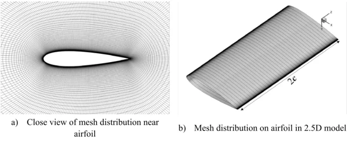
Both O- and C-grid mesh topologies can minimize the skewness of a near-wall mesh and converge fast under a high-order discretization scheme. In this study, the O-grid topology was adopted because it can reduce grid number and avoid high aspect ratios of grids in the far wake. In order to resolve the laminar sublayer directly, the first grid spacing on the airfoil was determined to make y+ less than 1. Grid-stretching was limited to less than 1.08 in both streamwise and crossflow directions to ensure numerical stability. Figure 4 shows the final meshes in both 2D and 2.5D models. The 2.5D model differs from the 2D model in the sense that it extends the model in a spanwise direction for a certain length. A couple of translational periodic conditions were enforced on the top and bottom boundaries. The 2.5D mesh (Figure 4-(b)) consisted of 280 cells along the airfoil wall, 120 cells in the normal direction to the wall, and 40 cells uniformly distributed in the spanwise direction. The number of cells was determined through a grid refinement study. In addition, the block-structured quadrangular grids were smoothed to decrease mesh skewness and achieve better grid orthogonality.
2.1.2 Turbulence models
The incompressible Navier-Stokes equation is appropriate for solving the VAWT aerodynamics, because the resultant flow velocity is generally smaller than 0.3 times the Mach number. Stall, either static or dynamic, may occur in a rotating VAWT, and both are dominated by vortex separation and involve flow unsteadiness. Therefore, an unsteady fluid solver is necessary to investigate such kinds of flow.
The choice of turbulence models influences the computational results and the required computation resource. The RANS models are wildly used in turbulence modeling with fair
accuracy and efficiency. Among the various RANS models, the SST model [26] is the one
combining the k−ω and k−ε models based on the zonal blending functions. The SST
model is considered a promising approach for simulating flow with great adverse pressure gradients and separation [27]. Compared with RANS, LES is more computationally demanding, in which larger and boundary-dependent eddies are resolved directly through the governing equations, and the influences of smaller and more homogeneous eddies are taken into account by a sub-grid model [28]. However, LES is compatible with a wider range of turbulent flows than RANS model, as it retains the unsteady large-scale coherent structures. For example,
Cummings et al. [19], Gao et al. [21], and Li et al. [29] proved that LES is an effective tool for simulating unsteady separated flows. The Smagorinsky-Lilly model overcomes the limitation of the original Smagorinsky sub-grid model and is one of the best-known LES models [30, 31]. In this study, the URANS approach with the SST model and the LES approach with the Smagorinsky-Lilly model were examined and compared. The SST model was examined in both 2D and 2.5D simulations, but only 2.5D LES was presented because the 2D LES simulation may not be rational, given that large eddies are resolved from 3D Navier-Stokes equations by direct numerical simulation (DNS) in LES. The results of 2D LES displayed a significantly inconsistent performance in different situations. The limitation of 2D LES is outside the scope of this study, and thus is not discussed here. Furthermore, in order to avoid arbitrary adjustment of the transition points, all the turbulence models were used in a fully-turbulent mode, and hence the laminar and transitional effects in the leading-edge region of the airfoil were excluded.
2.1.3 Simulation setup
The segregated approach was selected to solve the discretized continuity and momentum equations, and a second order implicit formula was used for the temporal discretization. The SIMPLEC scheme was used to solve the pressure-velocity coupling. SIMPLEC converges faster than SIMPLE and is more stable than the pressure-implicit with splitting of operators (PISO) scheme when the computational time step is relatively small in LES [32]. In the SST model, the second-order upwind discretization scheme and third-order MUSCL discretization scheme were applied for pressure and other variables, respectively. In the LES model, the bounded central difference scheme was used for spatial discretization of the momentum. As a result, the solutions were second-order accurate in the space and time domains. The steady state solution of the SST flow field was used as the initial condition of LES to accelerate the convergence.
Time step size is a crucial parameter in unsteady flow simulations. To get accurate results of an airfoil beyond stall, Sørensen et al. [20] and Travin et al. [22] suggested the non-dimensional time steps τ =ΔtU∞ /c to be 0.01 and 0.025 respectively. τ =0.0111 (corresponding to the real time step Δt=0.0001s) was applied in the simulations of the single airfoil. The flow was found to be statistically steady after 1 sec, and airfoil surface pressure was acquired in the following 2 sec, which was equal to 222 flow-through times according to the free stream velocity and airfoil chord length.
2.2 Results and Discussions
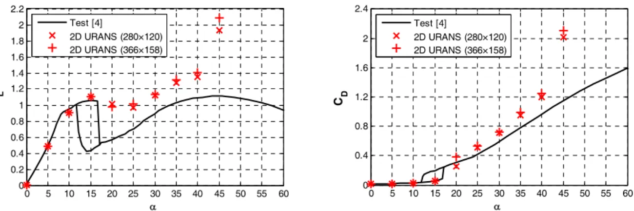
To achieve good tradeoff between computation accuracy and time requirement, a reasonable grid number was determined through a grid refinement study in the X-Y plane using the 2D model. Figure 5 shows the comparison of the results from two different mesh cases: 280×120 and 366×158. In general, the two cases showed good agreement with only a slight difference in post-stall AOAs, although both cases substantially deviate from the experimental results in the post-stall conditions. Therefore, the plane mesh size 280×120 was adopted hereinafter.
In the 2.5D model, the airfoil was extended in a spanwise direction in order to reproduce 3D turbulence structures. Too small spanwise width makes the flow become virtually 2D rather than 3D [23, 33]. At a low AOA, a relatively short spanwise width (e.g. 0.074c)is sufficient to obtain results comparable with wind tunnel data [34]; whereas in high AOA flow, a much longer width is needed to capture the larger 3D turbulence vortex separation and shedding structures. According to Johansen et al. [33] and Bertagnolio et al. [23], the spanwise width of 2c was selected in the 2.5D simulations in this study. To determine the most economical mesh, the mesh size in the spanwise direction was determined through a grid sensitivity study. The 2D mesh (280×120) was extruded to a fixed width of 2c with 20, 40 and 64 layers, respectively, in the spanwise direction. Figure 6 shows the comparison of three different 2.5D meshes in the LES simulations. It can be seen that the 20-layer mesh provided poor prediction of the lift force even at low AOAs; results of the 40-layer and 64-laryer meshes were almost similar, implying that a 40-layer mesh is capable of reflecting 3D flow structures. Thus, the mesh with 40 layers in the spanwise direction was adopted in the 2.5D CFD simulation in this study.
One of the objectives of this study is to verify the capability of 2.5D LES in simulations of VAWT aerodynamics. As pointed out in Section 1, the airfoils frequently encounter very high AOA flow, especially in the startup stage. Therefore, AOAs ranging from 0° to 140° were simulated using the aforementioned CFD strategies. The CFD simulations of airfoils at such high AOAs have been rarely reported in the literature, as they are not common in the application of general aerodynamic or hydrodynamic vehicles.
As the 2.5D LES was performed in a fully turbulent mode, it could not accurate depict the transition flow with laminar separation bubbles that may occur for clean airfoils at low Reynolds numbers. Delft University of Technology [4,25] conducted wind tunnel tests of both the clean and tripped NACA0018 airfoils, where zig-zag tapes were attached to the tripped airfoil to reduce or eliminate laminar separation bubbles. Figure 7 shows the comparison of the lift coefficients from the wind tunnel tests, as well as the 2.5D LES simulation. The results for the clean airfoil show a “kink” at α = 8̊ due to the laminar separation effect, which cannot be observed in the case of the tripped airfoil. For the aforementioned reason, the simulation results agree better with the experimental results for the tripped airfoil, although the tape thickness was not modeled in the 2.5D LES. Apart from the slight deviation at around 8̊, the lift coefficients of the clean and tripped airfoils coincide with each other well. Therefore, the influence of laminar separation should be minimal on the total power estimation of the VAWT investigated in this study.
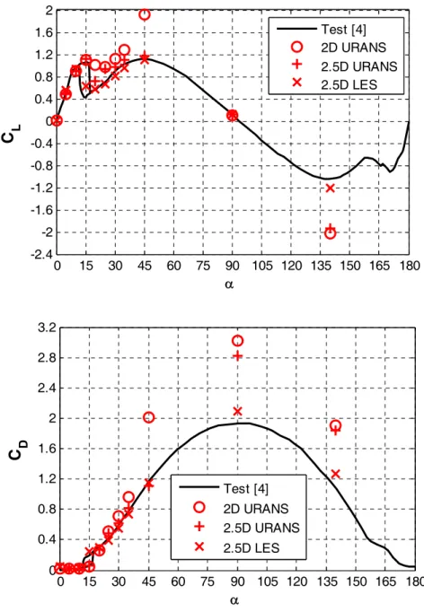
In addition to 2.5D LES, 2D URANS and 2.5D URANS simulations were also performed and compared with 2.5D LES in order to better understand the capability of 2.5D LES. Figure 8 shows the results of the mean lift and drag coefficients for the studied NACA 0018 airfoil obtained in 2D URANS, 2.5D URANS and 2.5D LES, as well as the wind tunnel test results obtained by Claessens [4]. Both the computational and experimental Reynolds numbers were equal to 300,000, which is close to that in the VAWT rotational flow studied in the next section. The stall starts at 12° and ends at 17°. In this process, the separation is initiated at the trailing edge of the airfoil and shifts forward to the leading edge with increasing AOA, whereas the lift force is kept almost constant. The wind tunnel results show a hysteresis loop caused by a deep stall, which may have been induced by the slow rolling of the airfoil section in the wind tunnel experiments. In our CFD simulations, the airfoils at different AOAs were completely static, and thus no such a hysteresis loop could be observed. This may also explain the difference between the 2.5D LES and experimental results at an AOA of 15°. At low (pre-stall) AOAs, both 2D and 2.5D URANS computations using the SST turbulence model agree with the experimental results well; however, at high (post-stall) AOAs, 2D URANS results in considerable over-prediction in both lift and drag. Although 2.5D URANS produces a significantly improved prediction of lift until 90° compared with 2D URANS, its drag coefficients substantially deviate from the experimental results at α = 90° and 140°. These results concur well with the conclusion by
Cummings et al. [19] that RANS models can provide accurate results for attached boundary layer flows but fail to simulate the large-scale turbulence in separated flows. Therefore, the URANS model, either 2D or 2.5D, is not suitable for resolving flow if the AOA is greater than 15°, which often occurs when VAWTs operate in a TSR λ<4. Compared with the 2D and 2.5D URANS models, the 2.5D LES shows an excellent agreement with the wind tunnel results from 0° to 140°. Its numerical error slightly increases with growing unsteady separation scale and flow uncertainties.
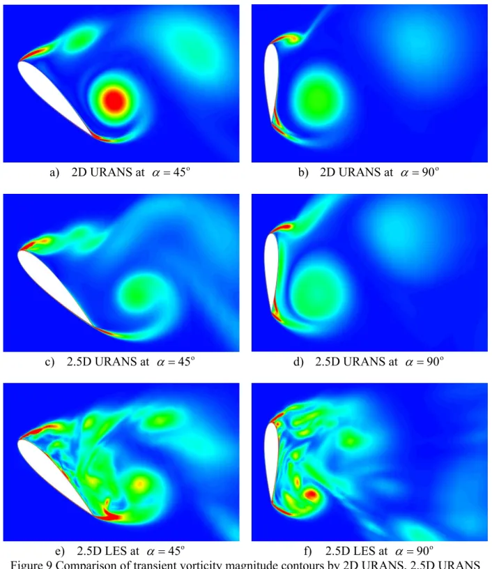
Figure 9 shows the transient vorticity contours at α = 45° and 90° from 2D URANS, 2.5D
URANS, and 2.5D LES simulation at the mid-span plane. Both 2D and 2.5D URANS produced large and smooth vortex shedding and prevented the vortices from diffusing into smaller ones, whereas the 2.5D LES computation reproduced the breakup of these large separation bubbles. This is consistent with the observations by Sørensen et al.[20] in the simulations of a flat plate. According to the incompressible vorticity transport equation, vorticity ω in a real flow is generated from the wall and diffused through fluid viscosity in all three directions. In 2D flow, however, vorticity diffusion is only valid in plane, which results in concentration in massive separation vortices. On the other hand, the RANS method is intended for modeling the turbulence by Reynolds time-averaged treatment, in which the Reynolds-stress term, regarded as energy transported through turbulence fluctuation, is unresolved but modeled using time-averaged terms. Therefore, it is unsurprising that only large periodic vortices shedding are reproduced by URANS.
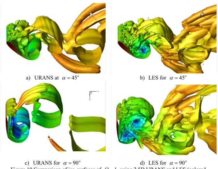
In order to illustrate the three-dimensionality of the flow, the vortex structures were identified and visualized using the Q-method [35]. Figure 10 shows the Q=1 iso-surfaces for the 2.5D URANS and LES. The URANS simulations remained almost two-dimensional in such highly separated flows, whereas the 2.5D LES could capture the essential pattern of the 3D flow. These
findings are supported by the pressure coefficient distribution over the airfoil (Figure 11). Since periodic boundaries were enforced at the two ends of the domain in the spanwise direction, the actual spanwise variation in average pressure is almost negligible. At α = 90°, the incorrectly diffused large vortices in the 2D and 2.5D URANS lead to too large suction pressure on the downwind surface of the airfoil, which consequently affects the lift and drag coefficients.
In summary, the poor accuracy of 2D and 2.5D URANS in the simulation of high AOA flow depicts that they may not be appropriate CFD tools in the aerodynamics study of VAWTs. McLaren [11] simulated static airfoil aerodynamics using a 2D steady-state CFD solution, and obtained acceptable results under AOAs ranging from 0° to 90°. However, the steady solver is not suitable in the study of VAWT aerodynamics, considering that stall is an unsteady phenomenon in physics and that our objective is to reproduce the unsteady flow in rotating VAWTs.
3
2.5D LES of 3-blade SBVAWT
3.1 Description of 3-blade SBVAWTMcLaren (2011) carried out a series of wind tunnel tests of a 3-blade SBVAWT at McMaster University. The blades employed NACA0015 airfoils with a round trailing edge. In particular, the transient tangential and normal forces acting on the blades were obtained through well-designed measurement instruments and post-processing of the test data. These experimental results provided valuable basis for the validation of CFD studies on VAWT aerodynamics. It should be noted that different airfoils—NACA0018 and NACA0015—were used in Sections 2 and 3, respectively. It is simply because of the limited availability of wind tunnel results for single airfoils and 3-blade VAWTs. Both NACA0018 and NACA0015 are widely used blade
sections in VAWTs [4, 36, 37], and they have similar aerodynamics. Thus, the previous
conclusions based on NACA0018 can provide deep insight into the VAWT performance assessment presented in this section.
3.2 CFD Simulation Strategy
3.2.1 Mesh geometry and boundary conditions
Figure 12 shows the geometry and flow conditions of the VAWT model in the CFD simulations, which are identical to the experimental setup in McLaren [11]. The radius of the VAWT was
m 4 . 1
=
R . A velocity inlet with a constant wind speed U=10 m/s was located 14m (i.e., 10R) in
front of the turbine. Outlet was placed 33.6 m (24R) behind the turbine to ensure full
development of wake flows. The applied outflow condition combined a zero diffusion flux for all flow variables in the normal direction to the exit plane and an overall mass balance correction. The side boundaries were 7m (5R) from the turbine center to minimize the blocking effects. A free-slip wall boundary condition was applied, where the normal velocity components and the normal gradients of all velocity components were assumed to be zero. The plane size of the computation domain was determined based on the principle that further increase of the domain
in 2D simulations leads to minimal variation in flow pattern and loads. Similar to the simulations of the single static airfoil, the 2.5D numerical VAWT model was obtained by vertically extruding the 2D mesh by 0.82m, which corresponds to twice the blade chord of the VAWT (Figure 13). Translational periodic conditions were applied on the top and bottom boundaries. As a result, the 2.5D model essentially represents a VAWT with an infinitely long blade, and the influences of finite span or tip vortices were not taken into account in this model. To increase the strength of the blade, Mclaren [11] employed a modified NACA0015 airfoil with a rounded trailing edge in his wind tunnel tests of VAWT. The modified chord length of the blades was 420 mm, rather than 450 mm of a standard NACA0015 airfoil. The mounted position of the supporting arms was offset from the leading edge by 150 mm, leading to an effective preset pitch angle of the blade β =2.66o, supposing that the pitch angle is defined as 0° when the blades are mounted at the mid-chord position [11]. Identical blade sections were modeled in this CFD study. For simplification, no supporting arms of the blades were modeled.
As shown in Figure 12, the whole computation domain was divided into three zones, namely zone A, zone B and zone C. Inner zone A and outer zone C were stationary, while zone B was a rotating ring separated from the two other zones by two non-conformal grid interfaces specified by sliding mesh boundary conditions. To avoid flow discontinuity on the interfaces, the ratios of the node spacing on the two sides of the interfaces were restricted to less than 2. A rotor shaft with a diameter of 0.1 m was also modeled in the center of zone A. The geometry, interface, and boundaries of the 2.5D model are shown in Figure 13.
After systematic minimization of the numerical uncertainties, the optimal mesh configurations used in the CFD model of the single static airfoil were transferred into the VAWT model with new boundary adaption (shown in Figure 14). The total number of grids in the 2D VAWT model was 131,690. In the 2.5D simulations, the 2D mesh was extruded by 0.82 m with 40 layers in the Z-direction, resulting in a grid number of 5,267,600. The real turbine blades in the experiment were 3m long, and a full 3D CFD model of the entire VAWT will result in a grid number at least fourfold of the current number in the 2.5D model if the 3D turbine domain is to be resolved accurately using a hexahedron-type mesh. Such a full 3D CFD model of the turbine is highly computationally intensive, and simulation of several revolutions may take a few months, excluding the time for flow initialization and convergence to a periodic solution.
3.2.2 Turbulence models and simulation setup
Similar to simulations of the single static airfoil, the 2D and 2.5D URANS approaches with the SST turbulence model and the 2.5D LES approach with the Smagorinsky-Lilly turbulence model were investigated and compared in this section. The dynamic stall of the blades influenced the primary energy extraction process of VAWT, and thus determination of the time step should consider amplitude, frequency and far field velocity. With the Reynolds number Re = 105,
Gharali et al. [38] suggested using τ =0.1 for the reduced frequency k =Ωc/2U∞ =0.026, and τ =0.01 for k =3.4. In the present study, the reduced frequency isk =0.1~0.3, the physical time step was 0.5oΩ−1 and the corresponding non-dimensional time step was τ =
0.02078. The simulation with a finer time step 0.25oΩ−1 was also conducted for the case of
96 . 1
=
λ , and the difference between two time steps was almost negligible. Thus, the adopted
time step 0.5oΩ−1 is believed to be small enough to obtain results independent with the time step size. To remove the initial effect, a total of six revolutions were simulated. In the final two revolutions, the numerical results differed by less than 2% from one revolution to another, which indicated the simulation reached a stable state. Therefore, all the data presented hereinafter are the average values of the final two revolutions.
3.3 Results and Discussions
The flow in the VAWT operating at a wind speed of 10m/s was simulated using 2D URANS, 2.5D URANS and 2.5D LES. Results were compared with the experimental results obtained by
McLaren (2011). The resultant aerodynamic forces acting on the blades were decomposed into two components—the normal force FN perpendicular to the chord and the tangential force FT parallel to the chord. Following [11], the tangential and normal force coefficients were defined as: cH U F C T T 0.5 2 ∞ = ρ (3) cH U F C N N 0.5 2 ∞ = ρ (4)
where H is the length of the blade. It should be mentioned that Mclaren [11] attempted to derive the aerodynamic tangential and normal force on the blade based on the measurements by the strain gauges mounted on the supporting arms. The measured normal forces were actually the superposition of the centrifugal and aerodynamic forces. It is difficult to accurately separate the aerodynamic normal force from the measurement results, as the centrifugal force fluctuated due to varying rotational speed and showed apparent variability from one test case to another. The final reported mean value of the experimental normal force was adjusted by McLaren [11] in orde to minize the discrepency in the mean aerodynamic normal forces between the experimental results and his 2D numerical simulations. Therefore, similar treatments were applied to the normal force in the experimental results again based on the 2.5D LES data in this study.
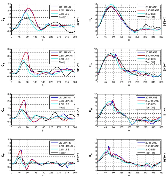
Figure 15 shows the comparison of tangential and normal force coefficients of the numerical and experimental results for four different TSRs, namely, λ = 0.7, 1.11, 1.46, and 1.96. In general, compared with the experimental results, the 2.5D LES provided a better prediction of the tangential force than 2D and 2.5D URANS, especially in the upwind zone (i.e., 0°< θ <180°). At a low TSR λ=0.7,the discrepancy in CT and CN values between the 2.5D LES results and the experimental results was quite small in terms of both peak magnitude and variation trend.
Such a low TSR often takes place in the starting process of VAWTs. This promising finding demonstrates that 2.5D LES can be an accurate and effective approach for evaluating the
self-starting characteristics of VAWTs. Similar to observations by other researchers [11, 13, 15], 2D and 2.5D URANS in this study tend to considerably overpredict the amplitudes of CT in the upwind zone. This is essentially due to the overprediction of lift forces in high AOA situations by 2D and 2.5D URANS. At high TSRs (λ>1.4), the discrepancy between the CFD simulations and experiments becomes relatively larger, but 2.5D LES still provides better
predictions of CT than 2D and 2.5D URANS. In normal force coefficients CN, all CFD
approaches lead to close approximation in general with regard to curve profiles and some principle values. One noteworthy fact is that the second peak torque in the downwind zone (180°<θ<360°) can be observed in the experimental results when λ = 1.46, 1.81 and 1.96. None of the three CFD approaches could reproduce this aerodynamic characteristic, which indicates that the CFD has limited capability in modeling vortices development and interaction with wake flow.
The amount of gross power P absorbed by a wind turbine in one revolution can be computed by
θ π π d 2 2 0
∫
Ω = NR FT P (5)where N is the number of blade. The turbine’s power coefficient CP is defined as the ratio of the turbine power output to the power available in the inflow
RH U P CP 2 5 . 0 3 ∞ = ρ (6)
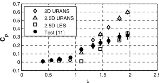
Figure 16 shows a plot of the power coefficient CP of the turbine as a function of TSR λ. The mean value of the wind tunnel results obtained by McLaren [11], together with the upper and lower bound corresponding to 14.5% error, is also presented. In general, the 2.5D LES not only properly predicted the variation trend of CP, but also was in reasonable agreement with the magnitudes of the wind tunnel results. The 2D and 2.5D URANS began to overestimate the power coefficient from λ=1.32, and this finding is consistent with those of other researchers. Figure 17 and Figure 18 shows a comparison of the power coefficients in the upwind and downwind zones, which offers deeper insight into the discrepency between the simulations and experiments. Because the maximum tangential forces are produced during the upwind revolution of the blades, the power coefficients in the upwind zone is much higher than that in the downwind zone. The blades in upwind zone extract more power from the more stable and energy-contained oncoming flow. In contrastr, the blades in downwind zone are located in the wake of the upwind blades and cannot efficiently extract power from the complex downwind flow.
Previous studies have reported the overprediction of power coefficients by 2D URANS. The discrepancy was often attributed to the effects of the tip vortices or flow divergence in real VAWTs. Results of this study indicate that, in general, 2.5D LES produces a more realistic
prediction of VAWT’s aerodynamic behavior than 2D URANS simulations. Because neither 2D URANS nor 2.5D LES can properly model the tip vortices or vertical flow divergence, the overprediction by 2D URANS is more likely the consequence of its inherent limitation in the prediction of lift force beyond stall. In view of the findings in the simulations of the single static airfoil, the inability to reproduce realistic large separations at high AOAs of the URANS model may be the major cause of the substantial difference between the URANS simulations and experiments, rather than the tip vortices and vertical flow divergence. Scheurich et al. [7] also illustrated the limited effect of tip vortices on the output power through the vorticity transport model.
Figure 19 shows deeper insight into the flow development of VAWT produced by 2.5D URANS and LES. According to Sheldahl et al. [17], when the Reynolds number is 360,000, the static stall of NACA 0015 airfoil starts at α = 13°, which corresponds to θ = 36° for λ=1.96 according to Eq. (2). As shown in Figure 19, dynamic stall delays the occurrence of the stall in VAWT, and consequently the lift does not drop until θ = 75° (corresponding to α = 25°). A series of vorticity magnitude and pressure contours around one blade at λ=1.96 are illustrated for various azimuthal positions in the upwind zone, including θ = 0°, 36°, 72°, 90°, 108°, 126°, 144°, 162° and 180°. When the blade rotates from 0° to 72°, the flow is always attached to the blade, and both lift and drag increase gradually with increasing AOA; the predicted vortical and pressure field by 2.5D LES and URANS are similar in this stage. Then, starting at θ = 72°, the clockwise vortices are significantly concentrated, and then shed from the leading edge region and gradually propagate over the airfoil surface, which causes pressure changes. As a result, the lift begins to significantly decrease and the blade is in the state of stall. Apparent discrepancy in the vorticity and pressure fields can be observed between 2.5D LES and 2.5D URANS, which explains the different peak tangential and normal forces predicted by these two methods in the upwind zone. 2.5D LES produces a clear phenomenon of shedding of clockwise vortices from the leading edge and developing along the inner surface of the blade, which was also observed in the particle image velocimetry (PIV) experimental results by Simão Ferreira et al.[39]. 2.5D URANS failed to capture the occurrence of dynamic stall vortices at high AOAs and delayed the stall of the blade, which resulted in the overprediction of the lift and power output.
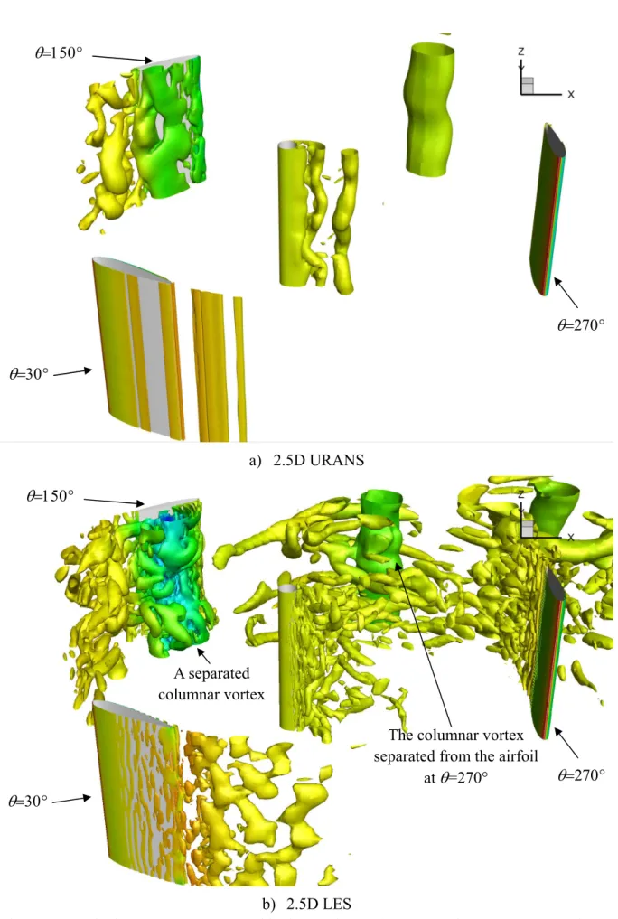
Figure 20 shows a transient vortical field from the 2.5D URANS and LES approaches for
λ=1.96. The 2.5D URANS simulated less vortices than the 2.5D LES because of its inherent treatment of Navier-Stokes equation. When the dynamic stall of the blades happens, the vortex shedding from the blades in the upwind zone has a crucial impact on VAWT energy extraction. As shown in Figure 20, the separated vortices in the dynamic stall follow a columnar shape, which induces a substantial pressure change but a relatively uniform pressure distribution along the vertical direction. However, the separations in the static stall (as shown in Figure 10-(a)) break into small vortices and yields pressure variation along the spanwise direction in the 2.5D URANS. This may account for the close prediction of aerodynamic forces in a rotating VAWT by 2D and 2.5D URANS when the dynamic stall of airfoil occurs, even though large differences exist in the static stall of a single airfoil.
4
Conclusions
This paper investigates the efficacy of the 2.5D LES approach in the aerodynamic study of SBVAWT. It is called 2.5D approach because only a short segment of airfoil blades in the spanwise direction was modeled, instead of building a 3D CFD model of the whole SBVAWT. A single static airfoil and an operating 3-blade SBVAWT were simulated using the 2.5D LES, and the results were compared with those obtained from wind tunnel experiments, as well as 2.5D and 2D URANS simulations. The comparisons demonstrated that the 2D URANS model considerably overpredicted the lift and drag of the single airfoil at post-stall AOAs due to the inaccurate vorticity diffusion behavior described by the 2D Navier-Stokes equation. 2.5D URANS can provide slightly improved results, but is also restricted by the capability of the URANS model for high AOAs flow containing large separations. Because high AOAs are very common to airfoil blades in an operating SBVAWT, the URANS model cannot offer an acceptable estimation of the output power of the SBVAWT. In contrast, 2.5D LES provided a much better agreement with the experimental results and a more realistic description of the aerodynamic details in both the single static airfoil and the rotating SBVAWT.
Researchers have recognized the deficiency of 2D URANS models in the aerodynamic study of VAWTs, but the deficiency used to be attributed to the negligence of tip vortices and vertical flow divergence in 2D simulations. However, the considerably improved prediction in 2.5D LES implies that these two factors may not be the main mechanism causing the overestimation by 2D URANS models. A careful inspection of aerodynamic details revealed that the URANS model delays the occasion of dynamic stall and overpredicts the tangential force in the upwind zones; in contrast, the 2.5D LES with an appropriate length in the spanwise direction can reproduce this dynamic flow pattern well. This inherent limitation of the URANS model explains its relatively poor accuracy in the performance assessment of VAWTs.
Findings of this study demonstrate that 2.5D LES is a more promising and efficient CFD tool to explore the aerodynamic characteristics of VAWTs. In the simulation of the 3-blade SBVAWT, 2.5D LES showed a good agreement with wind tunnel measurement at relatively low TSR. Hence, it can be employed in the study of the self-starting features of VAWTs, in which low rotation speeds and high AOAs are of main interest. At high TSR, 2.5D LES only offers fair agreement with the experimental results, although its performance is still better than that of the 2D and 2.5D URANS approaches. In particular, none of the three CFD approaches can well reproduce the tangential force in downwind zone at high TSR in this study. A high-fidelity CFD technique that can accurately model dynamic stall phenomena and highly separated flow in downwind zone needs to be developed in future aerodynamic studies of VAWTs.
Acknowledgements
The authors are grateful for the financial support from the Hong Kong Polytechnic University (Project No. A-PJ77 and 1-BB6X). Findings and opinions expressed here, however, are those of the authors alone, not necessarily the views of the sponsor.
References:
[1] I. Paraschivoiu, Wind turbine design: with emphasis on darrieus concept. 2002, Montréal, Québec, Canada: Polytechnic International Press.
[2] M. Islam, D.S.K. Ting and A. Fartaj, Aerodynamic Models for Darrieus-Type Straight-Bladed Vertical Axis Wind Turbines. Renew. Sustainable Energy Rev., 2008, 12(4) 1087-1109.
[3] W. Roynarin, Optimisation of Vertical Axis Wind Turbines. 2004, Northumbria University.
[4] M.C. Claessens, The design and testing of airfoils for application in small vertical axis wind turbines. 2006, Delft University of Technology.
[5] I.S. Hwang, Y.H. Lee and S.J. Kim, Optimization of cycloidal water turbine and the performance improvement by individual blade control. Appl. Energy, 2009, 86(9) 1532-1540.
[6] M.R. Castelli and E. Benini, Effect of Blade Inclination Angle on a Darrieus Wind Turbine. J. Turbomach., 2012, 134(3).
[7] F. Scheurich, T.M. Fletcher and R.E. Brown, The Influence of Blade Curvature and Helical Blade Twist on the Performance of a Vertical-Axis Wind Turbine, in 48th AIAA Aerospace Sciences Meeting Including the New Horizons Forum and Aerospace Exposition. 2010: Orlando, Florida, USA.
[8] B.K. Kirke, Tests on ducted and bare helical and straight blade Darrieus hydrokinetic turbines. Renew. Energy, 2011, 36(11) 3013-3022.
[9] M.H. Worstell, Aerodynamic Performance of the 17-Metre-Diameter Darrieus Wind Turbine. SAND78-1737. 1978, Sandia National Laboratories.
[10] R.E. Akins, P.C. Klimas and R.H. Croll, Pressure distributions on an operating vertical axis wind turbine blade element, in Proceedings of the American Solar Energy Society Annual Meeting, Sixth Biennial Wind Energy Conference. 1983. 455-462.
[11] K.W. McLaren, A Numerical and Experimental Study of Unsteady Loading of High Solidity Vertical Axis Wind Turbines. 2011, McMaster University.
[12] J.W. Oler, J.H. Strickland, B.J. Im, and G.H. Graham, Dynamic Stall Regulation of the Darrieus Turbine. SAND83-7029. 1983, Sandia National Laboratories.
[13] R. Howell, N. Qin, J. Edwards, and N. Durrani, Wind tunnel and numerical study of a small vertical axis wind turbine. Renew. Energy, 2010, 35(2) 412-422.
[14] M. Mukinovi, G. Brenner and A. Rahimi, Analysis of Vertical Axis Wind Turbines, in Numerical & Experimental Fluid Mechanics VII, NNFM 112. 2010. 587-594.
[15] M.R. Castelli, A. Englaro and E. Benini, The Darrieus wind turbine: Proposal for a new performance prediction model based on CFD. Energy, 2011, 36(8) 4919-4934.
[16] C.J. Simão Ferreira, A. van Zuijlen, H. Bijl, G. van Bussel, and G. van Kuik, Simulating dynamic stall in a two-dimensional vertical-axis wind turbine: verification and validation with particle image velocimetry data. Wind Energy, 2010, 13(1) 1-17.
[17] R.E. Sheldahl and P.C. Klimas, Aerodynamic Characteristics of Seven Symmetrical Airfoil Sections through 180-Degree Angle of Attack for Use in Aerodynamic Analysis of Vertical Axis Wind Turbines. SAND80-2114. 1981, Sandia National Laboratories.
[18] J. Rom, High angle of attack aerodynamics. 1992: New York: Springer.
[19] R.M. Cummings, J.R. Forsythe, S.A. Morton, and K.D. Squires, Computational challenges in high angle of attack flow prediction. Prog. Aerosp. Sci., 2003, 39(5) 369-384.
[20] N.N. Sørensen and J.A. Michelsen, Drag prediction for blades at high angle of attack using CFD. J. Sol. Energy Eng., 2004, 126(Nov.) 1011-1016.
low Reynolds numbers, in 46th AIAA Aerospace Sciences Meeting and Exhibit. 2008: Reno, Nevada.
[22] A. Travin, M. Shur, M. Strelets, and P.R. Spalart, Physical and numerical upgrades in the detached-eddy simulation of complex turbulent flows, Advances in LES of complex flows. 2004. 239-254.
[23] F. Bertagnolio, N.N. Sørensen and J. Johansen, Profile catalogue for airfoil sections based on 3D computations. Risø-R-1581(EN). 2006, Risø National Laboratory: Roskilde, Denmark.
[24] H. IM and G. Zha, Delayed Detached Eddy Simulation of a Stall Flow Over NACA0012 Airfoil Using High Order Scheme, in 49th AIAA Aerospace Sciences Meeting including the New Horizons Forum and Aerospace Exposition. 2011: Orlando, Florida.
[25] W.A. Timmer, Two-dimensional low-Reynolds number wind tunnel results for airfoil NACA 0018. Wind Eng., 2008, 32(6) 525-537.
[26] F.R. Menter, Two-equation eddy-viscosity turbulence models for engineering applications. AIAA Journal, 1994, 32(8) 1598-1605.
[27] F.R. Menter, M. Kuntz and R. Langtry, Ten Years of Industrial Experience with the SST Turbulence Model. Turbulence, Heat and Mass Transfer 4, 2003.
[28] J. Smagorinsky, General circulation experiments with the primitive Equations. I. The basic experiment. Mon. Weather Rev., 1963, 91(3) 99-164.
[29] C. Li, Q.S. Li, S.H. Huang, J.Y. Fu, and Y.Q. Xiao, Large eddy simulation of wind loads on a long-span spatial lattice roof. Wind Struct., 2010, 13(1) 57-82.
[30] M. Germano, U. Piomelli, P. Moin, and W.H. Cabot, A dynamic subgrid-scale eddy viscosity model. Phys. Fluids A: Fluid Dyn., 1991, 3 1760.
[31] D.K. Lilly, A proposed modification of the germano-subgrid-scale closure method. Phys. Fluids A: Fluid Dyn., 1992, 4(3) 633-635.
[32] Fluent Inc., FLUENT6.3 User's Guide. 2007.
[33] J. Johansen and N.N. Sørensen, Application of a detached-Eddy Simulation model on airfoil flows, in IEA2000. 2000.
[34] J. Winkler and S. Moreau. LES of the trailing-edge flow and noise of a NACA6512-63 airfoil at zero angle of attack. Center for Turbulence Research, Proceedings of the Summer Program. 2008.
[35] J. Joeng and F. Hussain, On the identification of a vortex. J. Fluid Mech., 1995, 285 69-94.
[36] A. Iida, K. Kato and A. Mizuno, Numerical Simulation of Unsteady Flow and Aerodynamic Performance of Vertical Axis Wind Turbines with Les, in 16th Australasian Fluid Mechanics Conference. 2007: Crown Plaza, Gold Coast, Australia.
[37] Y.M. Dai and W. Lam, Numerical study of straight-bladed Darrieus-type tidal turbine. Proceedings of the Institution of Civil Engineers, 2009, Energy 162 67-76.
[38] K. Gharali and D.A. Johnson, Numerical modeling of an S809 airfoil under dynamic stall, erosion and high reduced frequencies. Appl. Energy, 2011(doi: 10.1 016/j.ape nergy.2011.0 4.037).
[39] C. Simão Ferreira, G. van Kuik, G. van Bussel, and F. Scarano, Visualization by PIV of Dynamic Stall on a Vertical Axis Wind Turbine. Exp. Fluids, 2009, 46(1) 97-108.
o 0 = θ o 90 = θ o 180 = θ o 270 = θ m/s 10 = ∞ u r u ∞ u r Ω α 0 45 90 135 180 0 15 30 45 60 75 90 θ α λ=0.1 λ=0.5 λ=1.5 λ=2.0 λ=4.0
Figure 1 Schematic of the rotation of a 3-blade VAWT
Figure 2 Variation of AOA for different tip speed ratios Velocity Inlet U=22.2m/s Non-slip wall Velocity Inlet c=200mm R=30 c O X Y Z AOA, α Inflow direction
Figure 3 Geometry scheme and boundary conditions for single static NACA0018 airfoil
a) Close view of mesh distribution near
airfoil b) Mesh distribution on airfoil in 2.5D model
0 5 10 15 20 25 30 35 40 45 50 55 60 0 0.2 0.4 0.6 0.8 1 1.2 1.4 1.6 1.8 2 2.2 α CL Test [4] 2D URANS (280×120) 2D URANS (366×158) 0 5 10 15 20 25 30 35 40 45 50 55 60 0 0.4 0.8 1.2 1.6 2 2.4 α C D Test [4] 2D URANS (280×120) 2D URANS (366×158)
Figure 5 Comparison of mesh independence by lift and drag coefficients
0 5 10 15 20 25 30 35 40 45 50 55 60 0 0.2 0.4 0.6 0.8 1 1.2 1.4 1.6 α CL Test [4] 2.5D LES (280×120×20) 2.5D LES (280×120×40) 2.5D LES (280×120×64) 0 5 10 15 20 25 30 35 40 45 50 55 60 0 0.4 0.8 1.2 1.6 2 2.4 α CD Test [4] 2.5D LES (280×120×20) 2.5D LES (280×120×40) 2.5D LES (280×120×64)
Figure 6 Comparison of Z direction grids independence by lift and drag coefficients
0 5 10 15 20 25 30 0 0.2 0.4 0.6 0.8 1 1.2 α CL Test, Clean [4] Test, Trip at 70% [4] 2.5D LES
0 15 30 45 60 75 90 105 120 135 150 165 180 -2.4 -2 -1.6 -1.2 -0.8 -0.4 0 0.4 0.8 1.2 1.6 2 α C L Test [4] 2D URANS 2.5D URANS 2.5D LES 0 15 30 45 60 75 90 105 120 135 150 165 180 0 0.4 0.8 1.2 1.6 2 2.4 2.8 3.2 α C D Test [4] 2D URANS 2.5D URANS 2.5D LES
a) 2D URANS at α =45o b) 2D URANS at α =90o
c) 2.5D URANS at α =45o d) 2.5D URANS at α =90o
e) 2.5D LES at α =45o f) 2.5D LES at α =90o
Figure 9 Comparison of transient vorticity magnitude contours by 2D URANS, 2.5D URANS and 2.5D LES simulation at median-span plane as α =45o and α =90o
a) URANS at α =45o b) LES for α =45o
c) URANS for α =90o d) LES for α =90o
Figure 10 Comparison of iso-surfaces of Q =1 using 2.5D URANS and LES (colored according to pressure) 0 0.2 0.4 0.6 0.8 1 -3 -2 -1 0 1 2 x/c Me a n C P 2D URANS 2.5D URANS 2.5D LES Upwind surface 0 0.2 0.4 0.6 0.8 1 -3 -2 -1 0 1 2 x/c Me a n C P 2D URANS 2.5D URANS 2.5D LES Upwind surface a) α =45o b) α =90o
1.5R 0.5R R=10/3c 10R 5R 24R A B C Velocity inlet U=10m/s Outflow Free-slip wall Free-slip wall Non-conformal grid interface Rotor shaft Non-slip wall Blade Non-slip wall X Y Z c=420mm 0 = ∂ ∂ n φ 0 , ,yz = x τ 0 , ,yz= x τ
Figure 12 Scheme of geometry and boundary conditions for VAWT flow field simulation
Figure 13 Scheme of 2.5D model geometry and interface boundaries
a) Mesh around blade b) Mesh of rotational ring domain
c) Mesh for whole domain
0 45 90 135 180 225 270 315 360 -1 -0.5 0 0.5 1 1.5 2 2.5 3 3.5 θ C T λ =1 .9 6 2D URANS 2.5D URANS 2.5D LES Test [11] 0 45 90 135 180 225 270 315 360 -4 -2 0 2 4 6 8 10 12 θ C N λ =1 .9 6 2D URANS 2.5D URANS 2.5D LES Test [11] 0 45 90 135 180 225 270 315 360 -1 -0.5 0 0.5 1 1.5 2 2.5 3 3.5 θ C T λ =1 .4 6 2D URANS 2.5D URANS 2.5D LES Test [11] 0 45 90 135 180 225 270 315 360 -4 -2 0 2 4 6 8 10 12 θ C N λ =1 .4 6 2D URANS 2.5D URANS 2.5D LES Test [11] 0 45 90 135 180 225 270 315 360 -1 -0.5 0 0.5 1 1.5 2 2.5 3 3.5 θ C T λ =1 .1 1 2D URANS 2.5D URANS 2.5D LES Test [11] 0 45 90 135 180 225 270 315 360 -4 -2 0 2 4 6 8 10 12 θ C N λ =1 .1 1 2D URANS 2.5D URANS 2.5D LES Test [11] 0 45 90 135 180 225 270 315 360 -1 -0.5 0 0.5 1 1.5 2 2.5 3 3.5 θ C T λ =0 .7 0 2D URANS 2.5D URANS 2.5D LES Test [11] 0 45 90 135 180 225 270 315 360 -4 -2 0 2 4 6 8 10 12 θ C N λ =0 .7 0 2D URANS 2.5D URANS 2.5D LES Test [11]
Figure 15 Numerical and experimental tangential and normal force coefficients for λ=0.70, 1.11, 1.46 and 1.96
0 0.5 1 1.5 2 2.5 -0.1 0 0.1 0.2 0.3 0.4 0.5 0.6 0.7 λ C p 2D URANS 2.5D URANS 2.5D LES Test [11]
Figure 16 Power coefficients with tip speed ratio variation
0 0.5 1 1.5 2 2.5 -0.1 0 0.1 0.2 0.3 0.4 0.5 0.6 0.7 λ Cp 2D URANS 2.5D URANS 2.5D LES Test [11] 0 0.5 1 1.5 2 2.5 -0.1 0 0.1 0.2 0.3 0.4 0.5 0.6 0.7 λ Cp 2D URANS 2.5D URANS 2.5D LES Test [11]
Figure 17 Power coefficients in the upwind zone
Figure 18 Power coefficients in the downwind zone
0 600 1200 1800 2400 3000 -10 -7.5 -5 -2.5 0 2.5 5 θ =0° θ =36° θ =72° θ =90° θ =108° θ =126° θ =144° θ =162° θ =180°
2.5D LES 2.5D URANS 2.5D LES 2.5D URANS
(a) Contour of vorticity magnitude (b) Contour of pressure coefficient
Figure 19 Instantaneous contour of vorticity magnitude and pressure coefficient arount blade at 0°, 36°, 72°, 90°, 108°, 126°, 144°, 162° and 180° azimuthal positions for λ=1.96
a) 2.5D URANS
b) 2.5D LES
Figure 20 Vortical structures represented by iso-surfaces of Q=1000 of 2.5D URANS and LES results for λ=1.96 θ=30° θ=150° θ=270° A separated columnar vortex
The columnar vortex separated from the airfoil
at θ=270°
θ=150°
θ=30°