repository: http://orca.cf.ac.uk/115995/
This is the author’s version of a work that was submitted to / accepted for publication.
Citation for final published version:
Treder, Matthias S. 2018. Improving SNR and reducing training time of classifiers in large datasets
via kernel averaging. Lecture Notes in Computer Science file
Publishers page:
Please note:
Changes made as a result of publishing processes such as copy-editing, formatting and page
numbers may not be reflected in this version. For the definitive version of this publication, please
refer to the published source. You are advised to consult the publisher’s version if you wish to cite
this paper.
This version is being made available in accordance with publisher policies. See
http://orca.cf.ac.uk/policies.html for usage policies. Copyright and moral rights for publications
made available in ORCA are retained by the copyright holders.
Improving SNR and reducing training time of
classifiers in large datasets via kernel averaging
Matthias S. Treder1
School of Computer Science & Informatics, Cardiff University, Cardiff CF24 3AA, United Kingdom
Abstract. Kernel methods are of growing importance in neuroscience research. As an elegant extension of linear methods, they are able to model complex non-linear relationships. However, since the kernel ma-trix grows with data size, the training of classifiers is computationally demanding in large datasets. Here, a technique developed for linear clas-sifiers is extended to kernel methods: In linearly separable data, replacing sets of instances by their averages improves signal-to-noise ratio (SNR) and reduces data size. In kernel methods, data is linearly non-separable in input space, but linearly separable in the high-dimensional feature space that kernel methods implicitly operate in. It is shown that a clas-sifier can be efficiently trained on instances averaged in feature space by averaging entries in the kernel matrix. Using artificial and publicly available data, it is shown that kernel averaging improves classification performance substantially and reduces training time, even in non-linearly separable data.
Keywords: kernel·machine learning·big data·SVM·FDA
1
Introduction
In neuroscience, machine learning has been applied as a statistical tool for in-vestigating brain activity or structure, and as a computational model emulating brain activity [10]. In the first capacity, it has mostly been employed in the form of classifiers for applications such as multivariate analysis [7], classification of clinical data [13], and brain-computer interfaces [11]. Multivariate analysis of neuroimaging data poses several challenges, two of which are addressed here. Firstly, signal-to-noise ratio (SNR) in neuroimaging data is typically low [8]. Secondly, the increasing use of large-scale datasets [3] leads to unprecedented statistical power but also high computational demands for training a classifier.
Cichy and Pantazis [4] presented a simple technique that addresses both challenges at once. They had participants view images repeated 30 times each while MEEG was recorded. Trials from the same class were randomly partitioned into groups of 5, averaged tol=30/5=6 mean trials per class, and then used as input to a two-class linear Support Vector Machine (SVM). In [5] the authors averaged across groups of l = 40 trials. Obviously, averaging reduces the size
of the data by a factor of l, avoiding a bottleneck in classifier training time. In addition, averaging improves SNR substantially as evidenced by the high classification performance reported by the authors [4, 5].
As a linear operation, averaging only applies to linear classification tasks (see Fig. 1). Unfortunately, this precludes it from being used in kernel methods which can model more complex, non-linear relationships. Kernel methods are gaining popularity in social sciences [9] and in cognitive science [12], and they form the heart of the PRoNTo toolbox [15]. They are efficient when there is more variables than instances, such as in gene-expression data, since their complexity grows mainly with sample size [18, 14]. More recently, multiple kernel learning has been explored for the classification of fMRI and EEG data [20, 16].
The purpose of this paper is to extend the instance averaging approach of [4, 5] to kernel methods. The basic idea is simple: kernel methods are non-linear in the original input space, but they act as linear models in a high-dimensional feature space. Therefore, instances can be averaged in feature space rather than in input space. It is shown that the necessary computations can be efficiently carried out in input space using the kernel trick. The benefits of kernel averaging are two-fold: a smaller kernel matrix allows for reduced classifier training times and less memory consumption. At the same time, the averaging increases the SNR of the data and hence classification performance.
The paper is structured as follows. At first, classification and averaging are formally introduced. The effect of data averaging is discussed for the input space and the feature space and an efficient computation using the kernel trick is pre-sented. Subsequently, artificial data is used to illustrate that averaging instances in input space works for linearly separable data but not for linearly non-separable data, while kernel averaging works in both scenarios. Finally, four publicly avail-able datasets are used to evaluate the effects of kernel averaging on classification performance and classifier training time.
2
Method
Let the i-th instance in a dataset be denoted asxi ∈ X, where X is the input
space. Each instance has a corresponding class labelyi ∈ Y, whereY is the set of class labels. A classifier is a function f :X 7→ Y that maps an instance onto a predicted class label. For a binary classification task with class labels +1 and
−1, any linear classifier can be written in the form
f(x) = sgn(X i
αiyihxi,xi) (1) where the xi’s are the training instances, x is a test instance, sgn is the signum function, andh·,·iis the standard dot product [14].
2.1 The effect of averaging
Let instances from a given class be drawn from a probability distribution D
Data reduction in large datasets 3
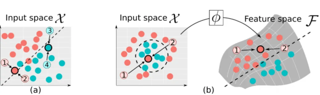
Fig. 1.Effect of averaging, illustrated for two classes (red and turquoise). (a) Linear classifiers use a linear decision boundary in input space (dashed line). When the red instances ”1” and ”2” are averaged (arrows), their average tends to be on the correct side of the hyperplane. The same applies to the turquoise instances ”3” and ”4”. (b)
Kernel classifiers use a non-linear decision boundary in input space (dashed circle). Averaging can pull the average onto the wrong side of the hyperplane even when the instances are on the correct side (see average of ”1” and ”2”). However, after projection into feature space usingφ, data are linearly separable.
towards the expectationE[x] in probability, that is,1
l
Pl
i=1xi
P
→E[x] asl→ ∞. Does a classifier applied to averages perform better than a classifier applied to the original instances? If the support of Dis a convex set, averaging can likely improve class separation (Fig. 1a). However, if it is non-convex, averaging can be detrimental. In extreme cases, the expected value occupies a part of input space wherein instances from this class are never observed, i.e.P(x=E[x] ) = 0. For instance, in Fig. 1b the turquoise class inhabits a circular region of input space. The region is convex so that averages remain within the circular region. However, the region inhabited by the red class is not convex and averages can end up within the circle although red instances are never observed there.
2.2 Averaging instances in input space
Cichy et al. [4, 5] averaged sets of instances prior to linear classification. Linear classifiers partition input space into convex regions so that averaging improves performance if the data is linearly separable. This can easily be demonstrated for the special case of a multivariate Gaussian distribution, i.e. xi ∼ N(m,Σ) with mean m and covariance matrixΣ. The distribution of the average across
l instances is 1
l
Pl
i=1xi ∼ N(m,Σ/l). In other words, the covariance matrix
is scaled down by a factor of l. Since it is usually conceived of as the noise, averaged instances move closer to the class mean, increasing class separability. This approach is referred to as instance averaging in the rest of the paper.
2.3 Averaging instances in feature space
Kernel classifiers partition input space into potentially non-convex regions. The data is implicitly projected to a high-dimensionalfeature space Fby applying a
functionφ:X 7→ F. A linear classifier is then applied inF. The formula in Eq. (1) applies when replacingxbyφ(x):
f(x) = sgn(X i
αiyihφ(xi), φ(x)i). (2) In other words, a kernel classifier acts as a linear classifier in feature space. Therefore, it is permissible to perform instance averagingin feature space. Next, an efficient way for averaging in feature space is developed.
IfFis associated with a Reproducing Kernel Hilbert space, dot products inF
can be represented by a kernel functionk:X × X 7→R,k(x,x′) =hφ(x), φ(x′)i. Crucially, this ’kernel trick’ can also be used in order to train a classifier on averages of instances in feature space. To see this, letz= [φ(x1) +φ(x2) +...+ φ(xl)]/l and z′ = [φ(x′1) +φ(x′2) +...+φ(x′l)]/l, l ∈N be two such averages. Then exploiting the bilinearity of the dot product one obtains
hz,z′i= 1 l2 X i,j∈{1,2,..,l} hφ(xi), φ(x′j)i= 1 l2 X i,j∈{1,2,..,l} k(xi,x′j). (3) Inserting this result into Eq. (2) yields a classifier trained on instances aver-aged in feature space. The quantity in Eq. (3) corresponds to a single entry in theaveraged kernel matrix. It is obtained by averaging several entries in the full kernel matrix. Therefore, this approach is referred to askernel averaging in the rest of the paper.
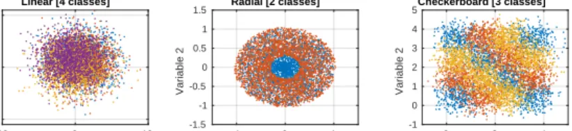
2.4 Artificial data -10 0 10 LDA 1 -5 0 5 LDA 2 Linear [4 classes] -1 0 1 Variable 1 -1.5 -1 -0.5 0 0.5 1 1.5 Variable 2 Radial [2 classes] 0 2 4 Variable 1 -1 0 1 2 3 4 5 Variable 2 Checkerboard [3 classes]
Fig. 2.Artificial datasets. The linear (Gaussian) dataset has been projected from 10 dimensions to the first 2 linear discriminant coordinates.
If the data is linearly separable, both instance averaging and kernel averaging should improve classification compared to no averaging. If the data is linearly non-separable, only kernel averaging should improve classification. To test this, three artificial datasets were generated and no averaging was compared to in-stance averaging and kernel averaging with groups ofl = 50 instances. ’Linear’ data was sampled from a multivariate Gaussian distribution in 10 dimensions.
Data reduction in large datasets 5
Four classes were created with different means but an equal covariance matrix sampled from a Wishart distribution. Two non-linearly separable datasets were generated in two-dimensional input space, a ’radial’ (2 classes) and a ’checker-board’ (3 classes) dataset. For each dataset, 6000 data points were created and Gaussian noise was added to every point. The datasets are depicted in Fig. 2.
2.5 Real data
To measure classification performance and computation time in real data, four publicly available datasets were analysed.
– EEG (http://bnci-horizon-2020.eu/database/data-sets). EEG from 11 par-ticipants performing an auditory oddball task [17]. Data were epoched in the interval [-0.2, 1] s and baseline corrected. Non-EEG channels were removed. To create a large dataset, trials from all participants were pooled, yielding 25,247 trials (instances), 63 variables (EEG electrodes), 241 time points, and 2 classes. Data was averaged in the typical interval for the P300 component (300–500 ms).
– Gene expression (http://archive.ics.uci.edu/ml/datasets/gene+expression+cancer+RNA-Seq). Part of the RNA-Seq (HiSeq) PANCAN dataset containing a random
extraction of gene expressions of patients having different types of tumor [19]. It totals 801 instances, 20,531 variables, and 5 classes.
– p53 mutants(http://archive.ics.uci.edu/ml/datasets/p53+Mutants). The dataset models mutant p53 transcriptional activity (active vs inactive) based on data extracted from biophysical simulations [6]. It totals 16,772 instances, 5409 variables, and 2 classes.
– Cardiotocography(http://archive.ics.uci.edu/ml/datasets/Cardiotocography). Fetal cardiotocograms with classes corresponding to morphologic pattern [1]. It totals 2126 instances, 23 variables, and 10 classes.
2.6 Analysis
All analyses were conducted using MATLAB R2017a (Natick, USA) on an Intel Core i7-6700 CPU 3.40GHz×8 computer with 64 GB RAM running on Ubuntu 18.04. Kernel Fisher Discriminant Analysis (FDA) and SVM were considered as
classifiers. For kernel FDA, an open-source implementation (https://github.com/treder/MVPA-Light/tree/devel) was used. For SVM, LIBSVM [2] was used. LIBSVM does not
implement kernel averaging, but it allows for pre-computed kernels to be pro-vided. For this reason, the kernel matrix was pre-computed for all analyses and manually averaged. The same kernel with the same hyperparameters was used for kernel FDA and SVM. For the simulations and the EEG and gene expression datasets, an RBF kernel was used. For the p53 mutants and the Cardiotocog-raphy datasets, a polynomial kernel was used. Hyperparameters were fixed to gamma=1/#variables, degree = 2, and coef0 = 0. All variables were z-scored.
Five-fold cross-validation was used to estimate classification accuracy. The procedure was repeated 10 times. Training time corresponds to the time it takes
to train a single classifier in one fold. Classification accuracy and training time were averaged across folds and repetitions. Its standard deviation was also cal-culated across folds and repetitions.
2.7 Complexity and memory
Kernel averaging reduces the size of the kernel matrix by a factor of l. The complexity implications are discussed for kernel FDA and SVM. The most com-putationally demanding part of kernel FDA is an inversion and an eigenvalue decomposition of n×n matrices at a complexity of O(n3
). It is reduced to
O(n3 /l3
) with kernel averaging. The complexity of the LIBSVM algorithm is reported as #iterations × O(n) if the n×n matrix can be cached [2]. Conse-quently, kernel FDA has a higher overall complexity than SVM and hence it should reap larger computational benefits from kernel averaging.
Memory consumption for storing the kernel matrix grows with n2
. For the largest dataset used in this paper (EEG data with 25,247 instances), the kernel matrix consumes about 2.3 GB RAM at single precision (4 bytes). The quadratic growth means that by just averaging 10 instances the memory required for the kernel matrix is reduced to about 23 MB, a factor of 100 smaller. The averaged kernel matrix can be built row-by-row or even entry-by-entry, so that the full kernel matrix is never actually required in memory.
3
Results
None Instance Kernel Averaging approach 0.0 0.2 0.4 0.6 0.8 1.0 Accuracy Dataset = Linear
None Instance Kernel Averaging approach
Dataset = Radial
None Instance Kernel Averaging approach Dataset = Checkerboard
Classifier kernel FDA SVM
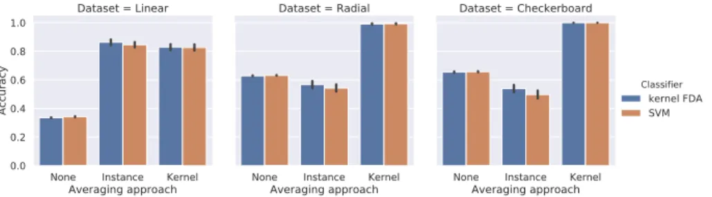
Fig. 3.Results on the artificial data. Similar results are obtained for kernel FDA (blue bars) and SVM (brown bars). When the data is linearly separable (Linear dataset), both instance averaging and kernel averaging improve classification performance. When the data is linearly non-separable (Radial and Checkerboard datasets), kernel averaging still improves classification performance but instance averaging does not.
Fig. 3 shows the results obtained on the artificial data. For linearly separable data, both instance averaging and kernel averaging improve classification perfor-mance from about 30% to about 80%. However, for the Radial and Checkerboard
Data reduction in large datasets 7 -0.2 0 0.2 0.4 0.6 0.8 1 Time [ms] 0.3 0.4 0.5 0.6 0.7 0.8 0.9 1 Accuracy None l=20 l=50
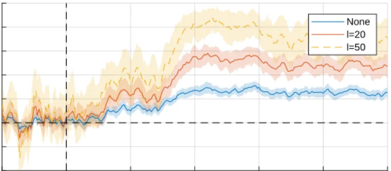
Fig. 4.Classification performance for participant #1 of the EEG dataset. Classification accuracy is plotted for every time point, comparing no averaging and kernel averaging withl= 20 andl= 50.
data, which are linearly non-separable, only kernel averaging leads to an improve-ment from about 60% to almost 100%. Instance averaging even has a slightly detrimental effect, leading to an accuracy<60%. Qualitatively, the same effects are observed for kernel FDA and SVM.
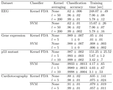
To illustrate the effect of kernel averaging on the EEG data, classification was performed for every time point for participant #1 using kernel FDA, comparing no averaging to kernel averaging withl = 20 andl = 50. Results are depicted in Fig. 4. Clearly, kernel averaging improves classification performance. For the rest of the analyses, EEG data was averaged in the 300-500 ms interval and all participants were pooled. Table 3 depicts the results for the 4 datasets. In all cases, kernel averaging leads to a consistent improvement of classification performance. For the EEG data, accuracy increases from 62% to 99%. For the Cardiotocography data, it increases from 88% to 98% (kernel FDA) and 91% to 99% (SVM). Even for the gene expression and p53 mutants datasets, kernel averaging improves performance although the classification is almost at ceiling to start with. The results are consistent across classifiers and kernels.
Kernel averaging also leads to a reduction of training time. This is especially evident for the two largest datasets, EEG and p53 mutants. In the EEG dataset, averaging l = 200 instances reduces training time from 248.07 s to 5.78 s for kernel FDA (40× faster), and from 15.67 s to 5.78 for SVM (3× faster). In the p53 mutants dataset, averagingl= 10 instances reduces training time from 151.25 s to 3.42 s for kernel FDA (40×faster), and from 4.17 s to 3.1 s for SVM (1.3×faster).
Dataset Classifier Kernel averaging Classification accuracy Training time [sec] EEG Kernel FDA None .62±.006 248.07±.49
l= 50 .96±.02 7.06±.08 l= 200 .99±.01 5.78±.12 SVM None .62±.01 15.67±.26
l= 50 .96±.02 7.06±.07 l= 200 .99±.002 5.78±.16 Gene expression Kernel FDA None .989±.007 .05±.04
l= 5 1±0 .01±.01
SVM None .988±.007 .008±.003
l= 5 1±0 .006±.002
p53 mutant Kernel FDA None .987±.002 151.25±25.52 l= 5 .993±.003 5.67±1.2 l= 10 .999±.002 3.42±.7 SVM None .9933±.0013 4.17±.65
l= 5 .9989±.0013 4.03±.67 l= 10 .9998±.0004 3.1±.53 Cardiotocography Kernel FDA None .88±.02 .635±.141
l= 5 .98±.01 .075±.024 SVM None .91±.01 .079±.019 l= 5 .99±.01 .057±.011
Table 1. Classification accuracy and training time for each of the 4 real datasets, classifier, and number of averages.
4
Discussion
An approach for averaging data in high-dimensional feature space has been de-veloped. The analysis of the artificial data shows that instance averaging (in input space) fails to improve classification performance when the data is linearly non-separable. In contrast, kernel averaging (in feature space) improves classi-fication performance for both linearly separable and non-separable data. This illustrates that kernel averaging is a genuine generalisation of averaging to non-linear input spaces. In fact, instance averaging arises as a special case of kernel averaging when a linear kernel is used.
The analysis of 4 real datasets reveals a consistent improvement of classifica-tion performance by kernel averaging. Even classificaclassifica-tion on the gene expression and p53 mutants datasets improves significantly, despite the fact that perfor-mance is close to 100% to start with. Furthermore, there is a consistent reduc-tion in training time. The benefit is most pronounced for kernel FDA with up to 40 times faster training on the EEG and p53 mutants datasets; smaller time benefits are obtained for SVM, in line with the complexity calculations.
Why not just subsample? For very large datasets, a simple alternative to kernel averaging is subsampling wherein just a subset of the data is selected. Because subsampling just discards large parts of the data, it does not offer the
Data reduction in large datasets 9
simultaneous improvement of SNR. However, if SNR is high to start with and performance is the only bottleneck, subsampling is a viable alternative.
How to interpret classification performance after averaging? If the classi-fier operates on averages rather than single instances, classification performance measures how wellgroups of instancescan be classified. This nicely dovetails with many neuroscience applications. Often, a typical question is whether the classi-fier can differentiate between a patient group and a control group, or whether trials wherein participants viewed a face can be classified from trials wherein they viewed a scene. Whether or not a classifier trained using kernel averaging is also beneficial in the original, single-instance classification setting, is a separate question that will be addressed in future research.
How many instances should be averaged? The present results suggest that even for moderate values of l, such as 5 or 10, a significant improvement in class separability is achieved. For low SNR data such as EEG, larger values for
l such as 20 or 50 can yield improvement without reaching ceiling performance. Conversely,l is bounded by data size. At least, l should be small enough such that a handful of averaged samples of each class occur in every training set.
Concluding, a novel kernel averaging approach has been developed that gen-eralises the notion of instance averaging to kernel classifiers. It allows for a significant improvement of SNR in conjunction with computational benefits, particularly for large datasets.
References
1. Ayres-de Campos, D., Bernardes, J., Garrido, A., Marques-de S´a, J., Pereira-Leite, L.: Sisporto 2.0: A program for automated analysis of car-diotocograms. The Journal of Maternal-Fetal Medicine 9(5), 311–318 (9 2000). https://doi.org/10.1002/1520-6661(200009/10)9:5¡311::AID-MFM12¿3.0.CO;2-9 2. Chang, C.c., Chang, C.c., Lin, C.j.: LIBSVM: A library for support vector
ma-chines. ACM Transactions on Intelligent Systems and Technology2(3), 1–27 (2011) 3. Choudhury, S., Fishman, J.R., McGowan, M.L., Juengst, E.T.: Big data, open sci-ence and the brain: lessons learned from genomics. Frontiers in human neuroscisci-ence
8, 239 (2014). https://doi.org/10.3389/fnhum.2014.00239
4. Cichy, R.M., Pantazis, D.: Multivariate pattern analysis of MEG and EEG: A comparison of representational structure in time and space. NeuroImage158, 441– 454 (9 2017). https://doi.org/10.1016/j.neuroimage.2017.07.023
5. Cichy, R.M., Ramirez, F.M., Pantazis, D.: Can visual information encoded in cor-tical columns be decoded from magnetoencephalography data in humans? Neu-roImage121, 193–204 (2015). https://doi.org/10.1016/j.neuroimage.2015.07.011 6. Danziger, S.A., Baronio, R., Ho, L., Hall, L., Salmon, K., Hatfield, G.W., Kaiser,
P., Lathrop, R.H.: Predicting Positive p53 Cancer Rescue Regions Using Most Informative Positive (MIP) Active Learning. PLoS Computational Biology 5(9), e1000498 (9 2009). https://doi.org/10.1371/journal.pcbi.1000498
7. Dima, D.C., Perry, G., Singh, K.D.: Spatial frequency supports the emergence of categorical representations in visual cortex dur-ing natural scene perception. NeuroImage 179, 102–116 (10 2018). https://doi.org/10.1016/J.NEUROIMAGE.2018.06.033
8. Gonzalez-Moreno, A., Aurtenetxe, S., Lopez-Garcia, M.E., del Pozo, F., Maestu, F., Nevado, A.: Signal-to-noise ratio of the MEG signal af-ter preprocessing. Journal of Neuroscience Methods 222, 56–61 (1 2014). https://doi.org/10.1016/J.JNEUMETH.2013.10.019
9. Hainmueller, J., Hazlett, C., Alvarez, R.M.: Kernel Regularized Least Squares: Reducing Misspecification Bias with a Flexible and Interpretable Machine Learning Approach. Political Analysis 22(2), 143–168 (2014). https://doi.org/10.1093/pan/mpt019
10. Hinton, G.E.: Machine learning for neuroscience. Neural Systems & Circuits1(1), 12 (8 2011). https://doi.org/10.1186/2042-1001-1-12
11. Hwang, H.J., Ferreria, V.Y., Ulrich, D., Kilic, T., Chatziliadis, X., Blankertz, B., Treder, M.: A Gaze Independent Brain-Computer Interface Based on Vi-sual Stimulation through Closed Eyelids. Scientific Reports 5, 15890 (10 2015). https://doi.org/10.1038/srep15890
12. J¨akel, F., Sch¨olkopf, B., FA Wichmann: Does cognitive sci-ence need kernels? Trends in cognitive sciences (2009), https://www.sciencedirect.com/science/article/pii/S1364661309001430
13. Orr`u, G., Pettersson-Yeo, W., Marquand, A.F., Sartori, G., Mechelli, A.: Using Support Vector Machine to identify imaging biomarkers of neurological and psy-chiatric disease: A critical review. Neuroscience & Biobehavioral Reviews36(4), 1140–1152 (4 2012). https://doi.org/10.1016/j.neubiorev.2012.01.004
14. Sch¨olkopf, B., Smola, A.J.: A Short Introduction to Learning with Kernels. In: Advanced Lectures on Machine Learning, pp. 41–64. Springer, Berlin, Heidelberg (2003). https://doi.org/10.1007/3-540-36434-X 2
15. Schrouff, J., Rosa, M.J., Rondina, J.M., Marquand, A.F., Chu, C., Ashburner, J., Phillips, C., Richiardi, J., Mour˜ao-Miranda, J.: PRoNTo: Pattern Recog-nition for Neuroimaging Toolbox. Neuroinformatics 11(3), 319–337 (7 2013). https://doi.org/10.1007/s12021-013-9178-1
16. Schrouff, J., Mour˜ao-Miranda, J., Phillips, C., Parvizi, J.: Decoding intracranial EEG data with multiple kernel learning method. Journal of Neuroscience Methods
261, 19–28 (3 2016). https://doi.org/10.1016/J.JNEUMETH.2015.11.028 17. Treder, M.S., Purwins, H., Miklody, D., Sturm, I., Blankertz, B.: Decoding auditory
attention to instruments in polyphonic music using single-trial EEG classification. Journal of neural engineering11(2), 026009 (2014). https://doi.org/10.1088/1741-2560/11/2/026009
18. Wang, X., Xing, E.P., Schaid, D.J.: Kernel methods for larscale ge-nomic data analysis. Briefings in bioinformatics 16(2), 183–92 (3 2015). https://doi.org/10.1093/bib/bbu024
19. Weinstein, J.N., Collisson, E.A., Mills, G.B., Shaw, K.R.M., Ozenberger, B.A., Ellrott, K., Shmulevich, I., Sander, C., Stuart, J.M., Stuart, J.M.: The Cancer Genome Atlas Pan-Cancer analysis project. Nature Genetics 45(10), 1113–1120 (10 2013). https://doi.org/10.1038/ng.2764
20. Youssofzadeh, V., McGuinness, B., Maguire, L.P., Wong-Lin, K.: Multi-Kernel Learning with Dartel Improves Combined MRI-PET Classification of Alzheimer’s Disease in AIBL Data: Group and Individual Analyses. Frontiers in human neuro-science11, 380 (2017). https://doi.org/10.3389/fnhum.2017.00380