Gradient test under non-parametric random effects models

(1)

Durham E-Theses

Gradient test under non-parametric random eects

models

MARQUES-DA-SILVA-JUNIOR, ANTONIO,HERMES

How to cite:

MARQUES-DA-SILVA-JUNIOR, ANTONIO,HERMES (2018) Gradient test under non-parametric random eects models, Durham theses, Durham University. Available at Durham E-Theses Online:

http://etheses.dur.ac.uk/12645/ Use policy

The full-text may be used and/or reproduced, and given to third parties in any format or medium, without prior permission or charge, for personal research or study, educational, or not-for-prot purposes provided that:

• a full bibliographic reference is made to the original source • alinkis made to the metadata record in Durham E-Theses • the full-text is not changed in any way

The full-text must not be sold in any format or medium without the formal permission of the copyright holders. Please consult thefull Durham E-Theses policyfor further details.

(2)

Academic Support Oce, Durham University, University Oce, Old Elvet, Durham DH1 3HP e-mail: [email protected] Tel: +44 0191 334 6107

http://etheses.dur.ac.uk

(3)

Gradient test under

non-parametric random effects

models

Antonio Hermes Marques da Silva J´

unior

A Thesis presented for the degree of

Doctor of Philosophy

Statistics and Probability Research Group

Department of Mathematical Sciences

University of Durham

England

(4)

Dedicated to

(5)

Gradient test under non-parametric random

effects models

Antonio Hermes Marques da Silva Junior

Submitted for the degree of Doctor of Philosophy

September 2017

Abstract

The gradient test proposed by Terrell (2002) is an alternative to the likelihood ratio, Wald and Rao tests. The gradient statistic is the result of the inner product of two vectors —

the gradient of the likelihood under null hypothesis (hence the name) and the result of

the difference between the estimate under alternative hypothesis and the estimate under null hypothesis. Therefore the gradient statistic is computationally less expensive than Wald and Rao statistics as it does not require matrix operations in its formula. Under some regularity conditions, the gradient statistic hasχ2_{distribution under null hypothesis.}

The generalised linear model (GLM) introduced by Nelder & Wedderburn (1972) is one of the most important classes of statistical models. It incorporates the classical regression modelling and analysis of variance either for continuous response and categorical response variables under the exponential family. The random effects model extends the standard GLM for situations where the model does not describe appropriately the variability in the data (overdispersion) (Aitkin, 1996a). We propose a new unified notation for GLM with random effects and the gradient statistic formula for testing fixed effects parameters on these models. We also develop the Fisher information formulae used to obtain the Rao and Wald statistics. Our main interest in this thesis is to investigate the finite sample performance of the gradient test on generalised linear models with random effects. For this we propose and extensive simulation experiment to study the type I error and the local power of the gradient test using the methodology developed by Peers (1971) and Hayakawa (1975). We also compare the local power of the test with the local power of the tests of the likelihood ratio, of Wald and Rao tests.

(6)

Declaration

The work in this thesis is based on research carried out at the Statistics and

Prob-ability Research Group, the Department of Mathematical Sciences, England. No part of this thesis has been submitted elsewhere for any other degree or

qualifi-cation and it is all my own work unless referenced to the contrary in the text.

“The copyright of this thesis rests with the author. No quotations from it should be

published without the author’s prior written consent and information derived from it should be acknowledged”.

(7)

Acknowledgements

The development of this thesis would not have been possible without the assistance

of several people, and it is impossible to acknowledge properly every individual contribution.

First and foremost I would like to express my sincere thanks to my main supervisor, Dr Jochen Einbeck, for his encouragement, interest and patience. Personally, I

would like to thank him for sharing his knowledge which has enriched my study in statistics. I have been extremely lucky to have a supervisor who cared so much

about my work, and who responded to my queries and questions so promptly and so fondly. His commitment and encouragement allowed me to present our work to

local and international conferences, where I became acquainted with the latest and greatest research and met many prestigious scientists.

I sincerely acknowledge my second supervisor Prof Peter Craig due to his continuous support, his kindness and always helpful and brilliant insights. His friendly guidance

and expert advice have been invaluable throughout all stages of the work.

I would like to take this opportunity to thank Prof Andrew Wood and Prof Michael

Goldstein – my viva examiners, for their very helpful comments and suggestions. I would also wish to express my gratitude to Prof John Hinde for receiving me at

NUI Galway, Ireland and valuable discussions which have contributed greatly to the improvement of this thesis.

I wish to thank to dozens of people at Department of Statistics of Universidade Federal do Rio Grande do Norte in Brazil who immensely helped me before and

during my PhD in UK. A special acknowledgement goes to my friends Dr Andr´e Pinho and Dr Carla Vivacqua who encouraged and support me before and through

(8)

vi

me to pursuit a degree outside Brazil.

I would like to acknowledge the financial support through the Brazil’s Science

With-out Borders Program grant nº 9622/13-6 from CAPES foundation.

Last but not least my parents Hermes and Evandir deserve my whole gratitude for

their immensely patience in raising me and for providing me the best care and love any parent could provide. I am deeply grateful to my wife Nat´alia and my daughter

Clarice for their immeasurable support, love and for the very happy moments.

(9)

List of Figures

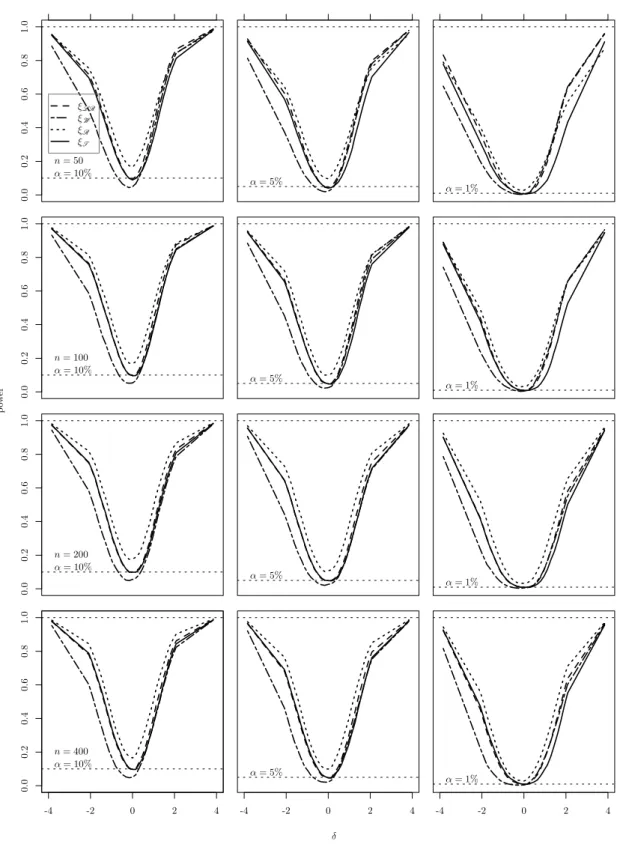
5.1 Non-null rejection rates of the four tests for Poisson response model

with Gaussian quadrature fitting and K = 3 . . . 62 5.2 Non-null rejection rates of the four tests for Poisson response model

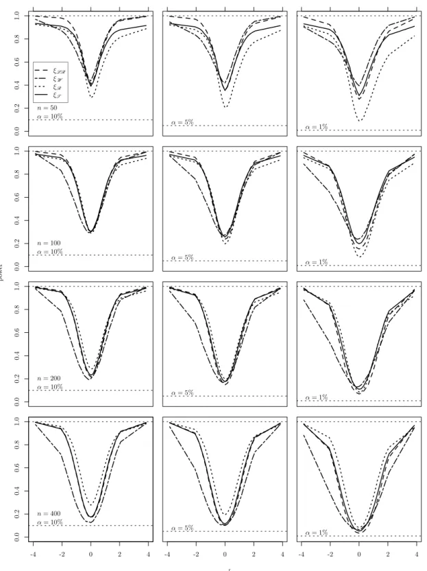
with NPML fitting and K = 3 . . . 65 5.5 Non-null rejection rates of the four tests for Poisson response model

with NPML fitting and K = 5 . . . 66 5.6 Non-null rejection rates of the four tests for Poisson response model

with NPML fitting and K = 7 . . . 67 5.7 Non-null rejection rates of the four tests for Poisson response variance

components model with NPML fitting and K = 3 . . . 68 5.8 Non-null rejection rates of the four tests for Poisson response variance

components model with NPML fitting and K = 5 . . . 69 5.9 Non-null rejection rates of the four tests for binomial response model

with Gaussian quadrature fitting and K = 3 . . . 70 5.10 Non-null rejection rates of the four tests for binomial response model

with NPML fitting and K = 3 . . . 73 x

(13)

List of Figures xi

5.13 Non-null rejection rates of the four tests for binomial response model with NPML fitting and K = 5 . . . 74 5.14 Non-null rejection rates of the four tests for binomial response model

with NPML fitting and K = 7 . . . 75 5.15 Non-null rejection rates of the four tests for binomial response

vari-ance component model with NPML fitting and K = 3 . . . 76 5.16 Non-null rejection rates of the four tests for binomial response

vari-ance component model with NPML fitting and K = 5 . . . 77 5.17 Non-null rejection rates of the four tests for gamma response model

with Gaussian quadrature fitting and K = 3 . . . 78 5.18 Non-null rejection rates of the four tests for gamma response model

with NPML fitting and K = 3 . . . 81 5.21 Non-null rejection rates of the four tests for gamma response model

with NPML fitting and K = 5 . . . 82 5.22 Non-null rejection rates of the four tests for gamma response model

with NPML fitting and K = 7 . . . 83 5.23 Non-null rejection rates of the four tests for gamma response variance

components model with NPML fitting and K = 3 . . . 84 5.24 Non-null rejection rates of the four tests for gamma response variance

components model with NPML fitting and K = 5 . . . 85 5.25 Non-null rejection rates of the four tests for normal response model

with Gaussian quadrature fitting and K = 3 . . . 86 5.26 Non-null rejection rates of the four tests for normal response model

with Gaussian quadrature fitting and K = 5 . . . 87 5.27 Non-null rejection rates of the four tests for normal response model

(14)

List of Figures xii

5.28 Non-null rejection rates of the four tests for normal response model with NPML fitting and K = 3 . . . 89 5.29 Non-null rejection rates of the four tests for normal response model

with NPML fitting and K = 5 . . . 90 5.30 Non-null rejection rates of the four tests for normal response model

with NPML fitting and K = 7 . . . 91 5.31 Non-null rejection rates of the four tests for normal response variance

components model with NPML fitting and K = 3 . . . 92 5.32 Non-null rejection rates of the four tests for normal response variance

components model with NPML fitting and K = 5 . . . 93 5.33 Non-null rejection rates of the four tests for inverse Gaussian response

model with Gaussian quadrature fitting and K = 3 . . . 94 5.34 Non-null rejection rates of the four tests for inverse Gaussian response

model with NPML fitting and K = 3 . . . 97 5.37 Non-null rejection rates of the four tests for inverse Gaussian response

variance components model with NPML fitting and K = 3 . . . 100 5.40 Non-null rejection rates of the four tests for inverse Gaussian response

variance components model with NPML fitting and K = 5 . . . 101 5.41 disparity values over iterations (left) and mass points estimates over

iterations (right) for the model in (5.2.11) fitted using allvc. . . 117 5.42 Bootstrap samples of the likelihood ratio statistic (left) and

gradi-ent statistic (right) compared to the theoretical χ2

2 for the test with

hypothesis H0 : (τ β)22 = (τ β)23= 0. . . 121

(15)

List of Figures xiii

5.43 Bootstrap power of the likelihood ratio test and the gradient test for nominal levels of 10% (left), 5% (center) and 1% (right). . . 121

5.44 90% confidence regions in black for (τ β)22 and (τ β)23 based on the

numerical inversion of the likelihood ratio test (left) and the gradient

(16)

List of Tables

4.1 Variance of response under Gaussian quadrature models. . . 38

4.2 Estimated fixed effects and respective standard errors (Poisson model with log link) . . . 41

4.3 Estimated fixed effects and respective standard errors (Gamma model with log link) . . . 42

4.4 Estimated fixed effects and respective standard errors (Normal model with identity link) . . . 42

4.5 Estimated fixed effects and respective standard errors (Inv. Gaussian model with inverse link) . . . 43

4.6 Estimated coverage probabilities (Poisson model with log link) . . . . 43

4.7 Estimated coverage probabilities (Gamma model with log link) . . . . 44

4.8 Estimated fixed effects and respective standard errors (strength data da Silva-J´unior et al. (2014)) . . . 45

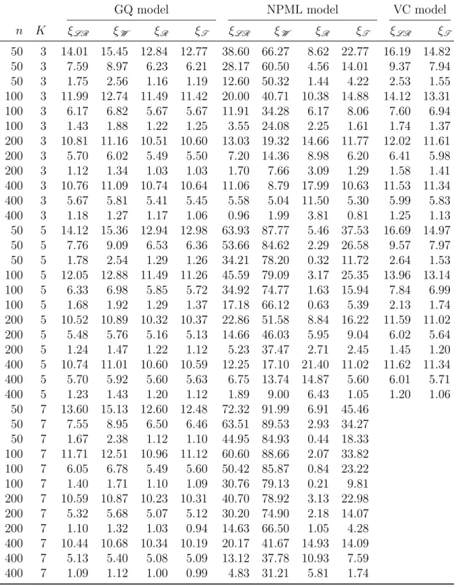
5.1 Monte Carlo standard errors for β˜3 and β˜4 for binomial models . . . . 50

5.2 Monte Carlo standard errors for β˜3 and β˜4 for Poisson models . . . . 51

5.3 Monte Carlo standard errors for β˜3 and β˜4 for gamma models . . . . 52

5.4 Monte Carlo standard errors for β˜3 and β˜4 for normal models . . . 53

5.5 Monte Carlo standard errors for β˜3 and β˜4 for inverse Gaussian models 54 5.6 Table of Figure enumerations for non-null rejection curves for each simulated scenario . . . 54

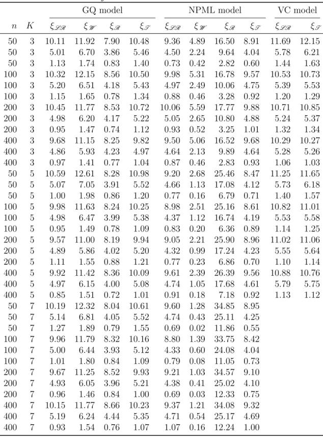
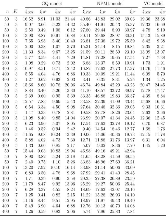
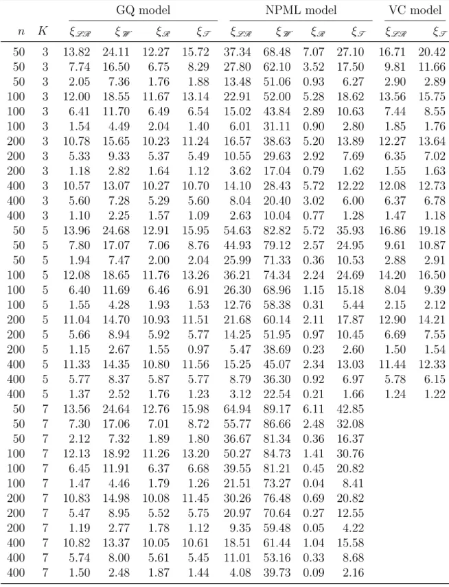
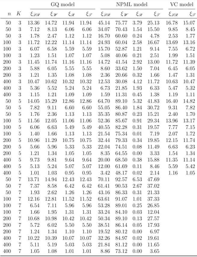
5.7 Null rejection rates of the four tests for Poisson models . . . 57

5.8 Null rejection rates of the four tests for binomial models . . . 58

5.9 Null rejection rates of the four tests for gamma models . . . 59

(17)

List of Tables xv

5.10 Null rejection rates of the four tests for normal models . . . 60 5.11 Null rejection rates of the four tests for inverse Gaussian models . . . 61

5.12 Results for testing H0 :β4 = 0 . . . 108

5.13 Factor allocation [source: Markussen (2017)]. . . 119

5.14 Likelihood ratio and gradient tests for the null hypothesis. Thep val-ues were computed using the chi-square distribution with two degrees

(18)

Chapter 1 Introduction

The gradient test is a relatively new asymptotic test proposed by Terrell (2002) as an alternative to the likelihood ratio, Wald and Rao tests. The gradient statistic is the inner product between two vectors — the gradient of the log-likelihood under

null hypothesis (hence the name) and the difference between the estimate under alternative hypothesis and the null hypothesis. Therefore, the gradient statistic

does not have any matrix or matricial operations in its formula, differently from the Wald and Rao statistics. This turns to be the most appealing advantage of the

gradient statistic, making it computationally less expensive than the aforementioned tests. The gradient statistic also is approximately chi-squared for sufficiently large

sample sizes and under some regularity conditions.

Since then, researchers have explored the finite sample properties of the gradient test

for several statistical models. Lemonte & Ferrari (2011b) studied the size and power in Birnbaum–Saunders regression model, Lemonte & Ferrari (2011c) studied testing

hypotheses in the Birnbaum–Saunders distribution under type-II censored samples, Lemonte & Ferrari (2011a) evaluated the local power of some tests in exponential

family nonlinear models, Lemonte (2012) studied the local power properties of some asymptotic tests in symmetric linear regression models, Lemonte & Ferrari (2012)

examined the local power and size properties of the LR, Wald, score and gradient tests in dispersion models, Vargas et al. (2013, 2014) proposes a Bartlett type

cor-rection for the gradient test, Lemonte (2013) developed the formulae of the gradient test for generalized linear models with dispersion covariates, Lemonte et al. (2012)

(19)

Chapter 1. Introduction 2

studied local power of the gradient test in comparison to the likelihood, Wald, Rao tests, Ferrari & Pinheiro (2014) evaluated the small-sample properties of the

gradi-ent test for extreme-value regression models and Medeiros et al. (2014) studied the performance of the gradient test for accelerated failure time models.

The random effect is a statistical concept conceived to accommodate an eventual extra variability due to unknown causes, such as omitted or unobserved variables,

measurement error or model misspecification. Models with random effects represent a flexible class through which overdispersion and variance component models can

be considered due to the special dependency structure in the variables. Given the stochastic nature of the random effects, we have to make assumptions concerning its distribution for inferential purposes. Notation-wise, lety be our sample and the marginal likelihoodm(y|θ) of the model with random effects represented by

m(y|θ) =

Z

f(y|θ, z)g(z)dz

where f(y|θ, z) is the conditional likelihood for the parameter θ which depends on the random effect z with unknown density g(z). This m(y|θ) is the likelihood of a mixture model(Aitkin, 1996a). The assumption of normally distributed random ef-fects is appropriate for many applications, but this also implies that the integration problem ofm(y|θ)is analytically solvable only for conjugated distributions. Numer-ical methods, such asGaussian quadrature (Golub & Welsch, 1969), are often used or the likelihood function is indirectly maximized.

The main issue of assuming any parametric distribution for the random effects is that this appears very artificial and is difficult to motivate in practice. If it is not

possible to make concrete assumptions about the distribution of the random effects, it would be useful to estimate the parameters alongside the density g( · ). A reference of this approach can be found in Anderson & Hinde (1988), where the iterative EM algorithm of Dempster et al. (1977) is used as an indirect method for

normally distributed mixtures of Poisson variable. Aitkin & Francis (1995) offer GLIM macros, which calculate the estimators for response distributions from

(20)

1.1. Organisation of the Thesis 3

analysis of overdispersion in generalised linear models (GLMs) is given in Anderson (1988) and Aitkin (1994, 1996a).

In this sense, assuming thatg( · )is unspecified, Laird (1978) proposed an estima-tion method called Nonparametric Maximum Likelihood (NPML) which consists in estimatingz and g(z) alongside toθ using an EM algorithm (Hinde, 1982).

Our main goal in this thesis is to evaluate the gradient test on the context of the

generalised linear models with random effects. We developed the unified formulae for the gradient test for the models with random effects with normal and unspecified

distribution. We performed an extensive Monte Carlo simulation experiment for verifying the type I and power of the gradient test for finite samples. We also

present numerical applications to real data sets.

1.1 Organisation of the Thesis

In organizing this thesis, we have divided the work in four main chapters. The

Chapter 2 establishes the background to this work, giving a comprehensive overview of the asymptotic theory for the likelihood based inference methods and tests. We

also express the general definition of the classic asymptotic tests and the gradient test.

In Chapter 3 we define the gradient statistic for testing parameters related to the fixed effects part of the model. For this we define, based on the literature, the

generalised linear model with random effects. We also propose a compact matrix notation not seen in the literature before. This notation helps in the development

of the R code use latter for simulation and application purposes.

In Chapter 4 we propose the formulae for the Fisher information for generalised

linear models with random effects. The proposed formulae includes an analytic method for the model with Gaussian random effects. We also propose an alternative

method based on the last EM algorithm estimates which can be applied for either models with Gaussian or unspecified distribution for the random effects. We provide

simulation results and an illustrative example. Although the gradient statistic does not use the Fisher information in its formula, we have developed it to obtain the

(21)

1.2. Spin-off publications 4

Wald and Rao statistics for comparison purposes in the Chapter 5.

In Chapter 5 we present an extensive simulation experiment to verify the finite

sample properties of the gradient test and compare to the likelihood ratio, Wald and Rao tests. This simulation covered various scenarios of the generalised linear models

with random effects including different sample sizes, response distributions, number of mass points and random effects distribution. We also provide four illustrative real

data examples for the gradient test.

The Chapter 6 concludes the thesis presenting an overview and discussing the

find-ings of this work.

The Appendix A present the functions in R code used to compute the tests and B

gives the analytic or approximated formulae to estimate the variance under the model with normal random effects.

1.2 Spin-off publications

Partial results of this thesis have been presented and published in the following conference proceedings.

• da Silva-J´unior, A. H. M., Einbeck, J. & Craig, P. S. (2015). The

gradient test for generalised linear models with random effects. In A. Blanco-Fernandez & G. Gonzalez-Rodriguez, eds., Programme and Abstracts: 9th In-ternational Conference on Computational and Financial Econometrics (CFE 2015) and 8th International Conference of the ERCIM (European Research Consortium for Informatics and Mathematics) Working Group on Computing & Statistics (ERCIM 2015). 63

• da Silva-J´unior, A. H. M., Einbeck, J. & Craig, P. S. (2016).

Gra-dient test on generalised linear models with random effects. In J.-F. Dupuy

& J. Josse, eds., Proceedings of the 31st International Workshop on Statistical Modelling, vol. 1. 213–218

• da Silva-J´unior, A. H. M. (2017). Gradient test for variance component

(22)

Inter-1.2. Spin-off publications 5

national Workshop on Statistical Modelling, vol. 2. 71–74

Chapter 4 is the outcome of a research project done together with Dr. Jochen Ein-beck and Prof. Peter Craig accepted for publication in

da Silva-J´unior, A. H. M.,Einbeck, J. & Craig, P. S. (2017). Fisher

infor-mation on Gaussian quadrature models. Statistica Neerlandica In press.

(23)

Chapter 2 Basics of likelihood inference and

the gradient test

2.1 Introduction

The method of maximum likelihood has been used extensively to estimate parame-ters in a large variety of models. The likelihood theory lends properties that allow

the formulation of asymptotic hypothesis testing, for instance, likelihood ratio (LR), developed by Wilks et al. (1938), followed by the Wald, (Wald, 1943) and Rao test

(Rao, 1948). Such tests have in common the χ2 as reference distribution for the sample sizen → ∞ and under the null hypothesis.

Recently, a new statistic was proposed by Terrell (2002) and has been calledgradient statistic orTerrell test. The gradient statistic is rather simple to compute and does not involve any matrix computations such as matrix products or inversions. The gradient statistic shares the same asymptotic properties of first order with the three

previous statistics. These features make the gradient statistic able to compete with the three well-established classical asymptotic tests.

We will suppose, initially, the following situation for the construction of the hy-potheses test. Let y = (y1, . . . , yn)> a sample of n independent observations of a random vector Y = (Y1, . . . , Yn)>, which has the pdf f( · ;θ) indexed by an un-knownp-dimensional vector of parametersθ = (θ1, . . . , θp)>. The likelihood function

(24)

2.1. Introduction 7

corresponding to the observed vector y from the density f(y,θ) is written

L(θ,y)≡L(θ) = f(y,θ) = n

Y

i=1

f(yi,θ).

and the log-likelihood function becomes

`(y,θ)≡`(θ) = n

X

i=1

logf(yi;θ). (2.1.1)

From (2.1.1) comes the score vector, the (observed) information matrix and the

Fisher information matrix defined, respectively, as

U(θ) = ∂`(θ) ∂θ> , J(θ) = − ∂U(θ) ∂θ> , and K(θ) = EhU(θ)U(θ)>i=−E " ∂U(θ) ∂θ> # = E[J(θ)].

The maximum likelihood estimator (MLE) is defined as the unique solution to

ˆ

θ= arg max

θ∈Θ

`(y;θ),

where θˆ = ˆθ(y) and, if it exists, usually can be obtained by solving the equation

U(θ) =0 also known as likelihood equations. In effect, the sufficient conditions to the existence and uniqueness of a MLE depend on the nature of both Θ and `(θ). IfΘis a compact space and `(θ) is continuous inΘ then there exists a MLE. Also, if the MLE exists, it is unique when Θ is a convex space and if `( · ,θ) is strictly concave in θ.

Important inferential tools for the MLE are obtained via Taylor series expansion of

`(θ) and U(θ) aroundθ0. In this sense, there are conditions to be verified in order

to discuss the asymptotic properties of the MLE and its functions. Such conditions

are often called regularity conditionsand will be presented in detail in Section 2.3.

(25)

2.2. Basic concepts of convergence 8

2.2 Basic concepts of convergence

First, let {Yn} be a sequence of random variables defined for a large n. Here n does not necessarily represent the sample size. We then present some important stochastic convergences that will be used on the next sections.

2.2.1 Convergence in probability

The sequence {Yn} converges in probability for a random variableY (which can be degenerate) if

lim

n→∞Pr(|Yn−Y|< ) = 1

for all >0. This convergence is denoted byYn P

→Y and means thatYn andY are approximately equal with probability close to 1 for a sufficiently large n.

2.2.2 Almost sure convergence

The sequence{Yn} convergesalmost surely to a random variable Y if

Pr lim n→∞Yn=Y = 1.

We denote this convergence by Yn

a.s. →Y.

2.2.3 Convergence in distribution

The sequence{Yn} converges in distribution toY if

lim

n→∞Pr(Yn< y) =FY(y),

for every y in IR where the distribution function FY( · ) of Y is continuous. We denote this convergence by Yn

D →Y.

(26)

2.3. Regularity conditions 9

2.2.4 Mann-Wald notation

The Mann-Wald notation is useful for describing the order of magnitude of specified quantities.

Let {an}∞n=1 be a sequence of positive values and {Yn}∞n=1 a sequence of random

vectors. We denote

Yn=Op(an) which means that a−n1Yn P

→0p, where0p is a vector in IRp, and

Yn=Op(an) which means that, for any > 0 there exist κ <∞ and n0 <∞ such

that, for all n > n0

Pr[ka−_n1Ynk> κ]< .

2.3 Regularity conditions

The following regularity conditions are used in asymptotic theory to justify and define the error terms of Taylor series expansions. Some of these conditions or

all of them are necessary to prove the asymptotic properties of the MLE such as consistency, normality and efficiency.

First, assume thatyis a realisation of a random vectorYwith distributionPθwhich

belongs to a classPand depends onθ ∈Θ. Also, the observationsy = (y1, . . . , yn)>, whereyi are iid with densityf(yi,θ)with respect to θ.

The following assumptions will be required further in this chapter:

(i) the distributions Pθ are distinct, i.e.,θ 6=θ0 implies Pθ 6=Pθ0;

(ii) the distributions f( · ,θ) have common support for all θ ∈ Θ, i.e., the set

Aθ ={y;f(y,θ)>0} does not depend on θ;

The condition (i) ensures that the probability distributions are different for distinct

θ and for the given data. The condition (ii) ensures that the sample space of y is identical and is independent ofθ.

Consider the observations y = (y1, . . . , yn)>, where yi are iid with density f(yi,θ) with respect toθ.

(27)

2.3. Regularity conditions 10

The assumptions (iii) and (iv) below ensure the regularity of f(y,θ) as function of

θ and the existence of an open set Θ1 in the parametric space Θ such as the true

parameterθ0 belongs to Θ1:

(iii) there exists an open set Θ1 ⊂ Θ which contains θ0 such that the density

function f(y,θ), for almost all y, which admits all the derivatives until third order in relation to θ, for allθ ∈Θ1;

(iv) Eθ[U(θ)] = 0 and the information matrix K(θ) is positive definite and has

finite values for all θ ∈Θ1;

(v) there are functions Mijk(y)which shall not depend onθ such that, fori,j and

k = 1, . . . , p, ∂3_f₍_y_;_θ₎ ∂θi∂θj∂θk <Mijk(y) for all θ ∈Θ1, where Eθ0[Mijk(Y)]<∞.

The condition (iii) represents the existence of Θ1 and the derivatives of f(y;θ)

until third order in Θ1. The condition (iv) ensures that the information matrix is

finite and positive-definite in an open neighbourhood of θ0. Finally, the condition

(v) ensures that the third order derivatives of the log-likelihood are bounded by a integrable function of Y whose expected value is finite (Cordeiro, 1999).

The models discussed on Chapter 3 make use of the mixture models theory from Aitkin (1996a) for modelling the random effects. In this sense, we have some

con-siderations about the regularity conditions stated above. According to Chen & Li (2009), the regularity conditions (i), (iv) and (v) are not always valid for Gaussian mixture models. We have then some undesired consequences such asunbounded likeli-hood function,loss of strong identifiabilityandinfinite Fisher information. However, this might not be an issue as we do not intent to test parameters regarding to the random effects.

On the other hand, fornon-parametric maximum likelihood mixture models, Lindsay (1995, chap. 1, pg. 24) makes the remark: ”one of the most striking features of the

above theory [Nonparametric maximum likelihood estimation] is the complete lack of regularity conditions on the models and the complete generality with regard to

(28)

2.4. Asymptotic properties of the MLE 11

2.4 Asymptotic properties of the MLE

2.4.1 Consistency

Commonly an estimator is considered a function of the sample sizen and, as long as we increase it (n→ ∞), we intuitively expect an enhance of the estimator precision.

Definition 2.4.1 Let y = (y1, . . . , yn)> be iid with density f(yi,θ) for each yi,

i= 1, . . . , n. Then, for n → ∞, an estimateθˆn = ˆθn(y) is consideredconsistent for the parameter θ if it satisfies

lim

n→∞MSE( ˆθn) = 0,

whereMSE( ˆθn) = E[( ˆθn−θ)>( ˆθn−θ)] is themean square error of θˆn.

In general, two definitions of consistency are widely used in asymptotic theory.

Definition 2.4.2 weak consistency: Let θˆn = ˆθn(y) the estimator for θ based on the iid sample y. Then, θˆn isweakly consistent if, for n → ∞

ˆ

θn=θ+Op(1).

Definition 2.4.3 strong consistency: Let θˆn= ˆθn(y)the estimator for θ based on the iid sample y. Then, θˆn isstrongly consistent if, for n→ ∞

Pr lim n→∞k ˆ θn−θk= 0 = 1.

This means that the weak or strong consistency happens whenθˆn satisfies the weak

law or the strong law of large numbers, respectively.

2.4.2 Normality

Theorem 2.4.4 Assume theiidsampley= (y1, . . . , yn)>with density f(yi,θ)and regularity conditions (i)–(v) valid. If θ˜ is a consistent solution for the maximum

(29)

2.4. Asymptotic properties of the MLE 12

likelihood equationsU(θ) = 0, then

√

n( ˜θ−θ0)

D

→Np(0,k(θ0)−1). (2.4.2)

In other words, for large sample sizes, the distribution of θ˜ is approximately p -dimensional normal with mean θ0 and covariance matrix K(θ0)−1 = n−1K(θ0)−1.

Cram´er (1999, Sec 33.3) and Lehmann & Casella (1998, Sec 6.4) show rigorous demonstrations of convergence of (2.4.2) for p= 1 and p_>1, respectively.

We shall demonstrate (2.4.2) for the uniparametric case. The general regularity conditions ensure the expansion of U(˜θ) = 0 around the true parameter θ0 up to

second order U(θ0) +U0(θ0)(˜θ−θ0) + 1 2U 00 (θ∗)(˜θ−θ0)2 = 0

where|θ∗−θ0|<|θ˜−θ0|and, therefore, θ∗ is necessarily consistent for θ0. The first

two terms on the left side of the equation are Op

n1/2 and the third is Op(1), as

U0(θ0) = Op(n), U00(θ0) = Op(n)and θ˜−θ0 =Op

n−1/2_{. The} _U₍_θ

0)and U0(θ0) are

sums of iidrandom variables so the expansion implies √ n(ˆθ−θ0) ( − n X i=1 Ui(θ0) nK(θ0) +Op n−1/2 ) = n X i=1 Ui(θ0) √ nK(θ0) .

where K(θ0) = n−1K(θ0) is the information of a single observation. By the weak

law of large numbers, Pn

i=1n−1U0(θ0)/K(θ0) = 1 +Op(1). Then, √ n(ˆθ−θ0){1 +Op(1)}= n X i=1 Ui(θ0) √ nK(θ0) . (2.4.3)

From (2.4.3) and the condition (iv), we can prove thatθˆhas asymptotic mean equal 0 and covariance structure given by K(θ0). Thus, the asymptotic normality of θˆis

obtained via central limit theorem applied to the right side of (2.4.3).

2.4.3 Efficiency

An estimatorθˆis considered asymptotically efficientfor θif it is consistent, asymp-totically normal and its covariance matrix is no larger than the covariance matrix

(30)

2.5. The gradient test and the classical asymptotic tests 13

of any other estimatorθ∗ ∈Θ which is consistent and asymptotically normal. The results of asymptotic efficiency and asymptotic normality can be generalised

for less restritive cases such as mixture models, provided that by week law of large numbersn−1_J₍_θ₎_→P _n−1_K₍_θ₎_{(Liang, 1984; Lindsay et al., 1991; Bickel et al., 1993).}

2.5 The gradient test and the classical asymptotic

tests

We present here the general idea of the gradient test proposed by Terrell (2002) and

its older sister tests, the likelihood ratio, Wald and Rao.

2.5.1 Simple hypothesis

Our chief concern will be testing the null hypothesis H0 :θ =θ0 against the

alter-native hypothesis Ha:θ 6=θ0 where θ0 is an arbitrary vector.

The definitions of the likelihood ratio, Wald and score test statistics for H0 are,

respectively,

ξLR= 2[`( ˆθ)−`(θ0)],

ξW= ( ˆθ−θ0)>K( ˆθ)( ˆθ−θ0),

ξR=U(θ0)>K(θ0)−1U(θ0),

where θˆis the maximum likelihood estimator (MLE) of θ, which can be obtained by U( ˆθ) = 0. A different approach for the Wald test is to substitute the Fisher

information matrix estimated under the alternative hypothesis by the theoretical equivalent under null hypothesis. Here, we will call this approach as modified Wald

statistic, and define as

ξMW= ( ˆθ−θ0)>K(θ0)( ˆθ−θ0).

Cordeiro (1999) shows that the asymptotic distributions of ξW, ξR and ξMWcan be

(31)

obtained considering that

√

nU(θ)→D Np(0,K¯(θ))

√

n( ˆθ−θ)→D Np(0,K¯(θ)−1).

whereK(θ) =nK¯(θ). If K(θ) is continuous in θ=θ(0) _{thus, for} _n _{→ ∞}_,

n−1J(θ(0))→P K¯(θ(0))

n−1J( ˆθ)→P K¯(θ(0)).

(2.5.4)

One can show that ξLR has chi-squared distribution using the Taylor expansion of

`(θ(0)₎ _{around the solution} _θˆ_from _U_{( ˆ}_θ_{) =}₀ _{and (2.5.4). Thus,}

`(θ(0)) =`( ˆθ) + *0 U( ˆθ)(θ(0)−θˆ)− 1 2(θ (0)₋_θ_ˆ₎> J( ˆθ)(θ−θˆ) +Op(1), =`( ˆθ)− 1 2(θ (0)₋_θ_ˆ₎>_K_{( ˆ}_θ₎₍_θ(0)₋_θ_ˆ_{) +} Op(1) or ξLR= ( ˆθ−θ(0))>K( ˆθ)( ˆθ−θ(0)) +Op(1). (2.5.5)

Likewise, the Taylor expansion forθˆaroundθ(0)

ˆ θ=θ(0)+K(θ(0))−1U(θ(0)) +Op n−1/2 ˆ θ−θ(0) =K(θ(0))−1U(θ(0)) +Op n−1/2 (2.5.6) Substituting (2.5.6) in (2.5.5), we have ξLR = [K(θ(0))−1U(θ(0))]>K( ˆθ)[K(θ(0))−1U(θ(0))] +Op(1) =U(θ(0))>[K(θ(0))−1]>K( ˆθ)K(θ(0))−1U(θ(0)) +Op(1),

where commonlyK(·) is a symmetric matrix, thenK(· )>=K(· )(also valid for its inverse) and by the strong consistency ofθˆ, K( ˆθ)→a.s. K(θ(0)_{), thus}

(32)

The statistics ξLR, ξW, ξR and ξMW have centred chi-square distribution approx-imately with p degrees of freedom (χ2

p) under the null hypothesis H0 : θ = θ0.

Therefore, we reject H0 if the observed value of the statistic exceeds the quantile

100×(1−α)% of the χ2

p distribution, with nominal level α.

We are now able to discuss the idea behind the gradient statistic. LetMp×p a square matrix that satisfies the conditionM>M=K(θ). Using this matrix, we can rewrite

ξR and ξMWas

ξR = [(M−1)>U(θ0)]>(M−1)>U(θ0),

ξMW= [(M)( ˆθ−θ0)]>M( ˆθ−θ0).

Lemonte (2016) shows that

(M−1)>U(θ0)∼Np(0,Ip),

M( ˆθ−θ0)∼Np(0,Ip), whereIp is a p-dimensional identity matrix.

Furthermore, the inner product between(M−1₎>_U₍

θ0) and M( ˆθ−θ0) results in

[(M−1)>U(θ0)]>M( ˆθ−θ0) =U(θ0)>M−1M( ˆθ−θ0)

=U(θ0)>( ˆθ−θ0).

Based on the last expression, we have the following definition:

Definition 2.5.1 (Terrell, 2002) The gradient statistic, ξT, to test the simple null hypothesis H0 :θ =θ0 against Ha:θ 6=θ0 has the form

ξT=U(θ0)>( ˆθ−θ0).

Theorem 2.5.2 Under H0 :θ =θ0, ξThas χ2p+Op(1) distribution.

Proof: The MLE θˆis asymptotically efficient under the regularity conditions and ˆ

θ−θ0 =K(θ0)−1U(θ0) +Op

n−1/2.

(33)

We already know that, in same conditions,

U(θ0) = Op

n1/2,

then

ξT=U(θ0)>( ˆθ−θ0) = U(θ0)K(θ0)−1U(θ0) +Op(1) =ξR.

Therefore, asξR has χ2p+Op(1) then ξThas as well. 2 Note that ξT has the advantage of not involving the estimated Fisher information matrix neither its inverse. We cannot state thatξTis non-negative for any scenario except for the case stated in the Theorem 2.5.3.

Theorem 2.5.3 (Terrell, 2002) If `(θ) is uni-modal and differentiable inθ, so

ξT=U(θ0)>( ˆθ−θ0)>0

Proof: Assuming the regularity conditions (i)–(v) and by the uniqueness of the MLE, θˆ is the only existent point of maxima of `( · ) and therefore, solution for

U( ˆθ) =0. Let exist a θ0 = (θ0₁, . . . , θ_p0)> ∈Θsuch that

U(θ0)>( ˆθ−θ0)<0,

i.e., a violation of the Theorem. Then, U(θ0) 6= U( ˆθ) = 0 and θ0 6= ˆθ. This means that only θ0 < θˆ or θ0 > θˆ might be true. If θ0_i < θˆi, for i in 1, . . . , p, then

U(θ_i0)<U(ˆθi) by the uni-modality of `( · ). As a consequence,

U(θ0)>( ˆθ−θ0)>0.

For the second situation, if θ0_i >θˆi, fori in 1, . . . , p, thenU(θ0i)>U(ˆθi) also by the uni-modality of`(· ). Thus,

U(θ0)>( ˆθ−θ0)>0.

(34)

2.5. The gradient test and the classical asymptotic tests 17 Example 2.5.1 Let y = (y1, . . . , yn)> a n size random sample from a Gaussian distribution with mean θ and variance 1, N(θ,1). Thus,

`(θ) = log " _n Y i=1 (2π)−1/2exp ( −(yi−θ) 2 2 )# =−n 2log(2π)− 1 2 n X i=1 (yi−θ)2,

which provides the uni-parametric versions of score and Fisher information, respec-tively U(θ) = n X i=1 yi−nθ, K(θ) = n.

so that for U(θ) = 0, the maximum likelihood estimator for θ isθˆ=Pn

i=1yi/n = ¯y. Consider the null hypothesisH0 :θ=θ0. For testingH0, the likelihood ratio statistic

assumes ξLR=2 " −n 2log(2π)− 1 2 n X i=1 (yi −y¯)2 + n 2log(2π) + 1 2 n X i=1 (yi−θ0)2 # = n X i=1 [(yi−θ0)2−(yi −y¯)2] = n X i=1 [ y 2 i −2θ0yi +θ02 −y_i2+ 2¯yyi−y¯2] =−2nθ0y¯+nθ20 + 2ny¯ 2₋_n_y_¯2 ₌_n_[¯_y2₋₂_θ 0y¯+θ20] =n(¯y−θ0)2.

Similarly, the Wald, Rao and gradient statistics are, respectively,

ξW= (ˆθ−θ0)2K(ˆθ) =n(¯y−θ0)2, ξR =U(θ0)2/K(θ0) = [n(¯y−θ0)]2/n =n(¯y−θ0)2, May 30, 2018

(35)

and

ξT=U(θ0)(ˆθ−θ0)

=n(¯y−θ0)(¯y−θ0)

=n(¯y−θ0)2.

Example 2.5.2 Let y = (y1, . . . , yn)> a n size random sample from a exponential distribution with pdf f(y;θ) = 1 θ exp −y θ . Thus, `(θ) = log " _n Y i=1 1 θ exp −yi θ # =−nlogθ− 1 θ n X i=1 yi.

which provides the respectively uni-parametric versions of score and Fisher

informa-tion U(θ) =−n θ + 1 θ2 n X i=1 yi, K(θ) = n θ2.

so that for U(θ) = 0, the maximum likelihood estimator for θ isθˆ=Pn

i=1yi/n = ¯y. Consider the null hypothesisH0 :θ=θ0. For testingH0, the likelihood ratio statistic

is ξLR= 2 " −nlog ¯y− 1 ¯ y n X i=1 yi+nlogθ0+ 1 θ0 n X i=1 yi # = 2n " log θ0 ¯ y ! + y¯ θ0 −1 # .

Similarly, the Wald, Rao and gradient statistics are, respectively,

ξW= (ˆθ−θ0)2k(ˆθ) =n(¯y−θ0)2 n ¯ y2 =n y¯−θ0 ¯ y !2

(36)

2.5. The gradient test and the classical asymptotic tests 19 ξR=U(θ0)2/K(θ0) = _n θ0 _y_¯ θ0 −1 2, _n θ2 0 ! =n y¯−θ0 θ0 !2 , and ξT=U(θ0)(ˆθ−θ0) =n y¯ θ2 0 − 1 θ0 ! (¯y−θ0) =n y¯ 2₋_yθ_¯ 0−yθ¯ 0+θ20 θ2 0 ! =n y¯−θ0 θ0 !2 .

2.5.2 Composite hypothesis

We now will consider the problem of testing the hypotheses

     H0 :θ1 =θ (0) 1 Ha:θ1 6=θ (0) 1 ,

which implies the partitioning θ = (θ₁>,θ₂>)> where θ1 = (θ1, . . . , θq)> is a q -dimensional parameter of interest, θ2 = (θq+1, . . . , θp)> is a (p − q)-dimensional nuisance parameter and θ₁(0) is a specified vector. Let `(θ1,θ2) the log-likelihood

for θ1 and θ2. The unrestricted maximum likelihood estimator is θˆ = ( ˆθ>1,θˆ

>

2)

>

and the restricted maximum likelihood estimator of θ2 under H0 is written θ˜2; so,

˜

θ> = (θ₁(0)>,θ˜>₂) represents the estimator of the full parameter vector θ under the null hypothesis. We make use for further formulae the mathematical accents∼and ∧to represent the estimators under null and alternative hypothesis, respectively. The score vectorU, the Fisher information matrixKand the inverted Fisher

(37)

mation matrixK−1 _{are also partitioned according to} _θ_{= (}_θ>

1,θ2>)>, i.e. U≡U(θ) =    U1 U2   , K≡K(θ) =    K11 K12 K21 K22   , and K−1 ≡K−1(θ) =    K11 _K12 K21 _K22   ,

Similarly, we can use the same notation for the observed information matrix J and

its inverse J−1_{. In general, the} _U

1, U2, K11, K12 = K>21 and K22 depend on both θ1 and θ2.

The likelihood ratio statistic for H0 :θ1 =θ (0) 1 is

ξLR= 2[`( ˆθ1,θˆ2)−`(θ (0)

1 ,θ˜2)]. (2.5.7)

The inconvenience of (2.5.7) is thatξLR requires two maximisations. One can show that ξLR

D →χ2

q according to Wilks et al. (1938).

The Wald statistic is developed on the basis of the asymptotic normality of the MLE ˆ

θ1. The idea is that the distribution ofθˆis, asymptotically, ap-dimensional normal

distribution, where K−1 is the covariance matrix. Thus, under H0, the asymptotic

distribution of θˆ1 is also normal, however, q-dimensional and with mean θ (0)

1 and

covariance matrixK11. This means that,θˆ1−θ (0) 1

D

→Nq(0,K11). The matrixK11can be consistently estimated byK11_{( ˆ}_θ 1,θˆ2),K11(θ (0) 1 ,θ˜2),J11( ˆθ1,θˆ2) andJ11(θ (0) 1 ,θ˜2).

If we choose the first option, the Wald statistic can be expressed by

ξW= ( ˆθ1−θ (0) 1 ) >_ˆ K11−1( ˆθ1−θ (0) 1 ) (2.5.8) where Kˆ11 ₌ _K11_{( ˆ}_θ

1,θˆ2). In (2.5.8), ξW is a “quadratic form” which corresponds to an inner product of a two vectors that have the same asymptotically normal

distributionθˆ1−θ1(0)

D

→Nq(0,K11) and, therefore,ξW D

→χ2_q under null hypothesis. The Rao statistic is based on the asymptotic normality for the score functionU1 =

(38)

U1(θ (0

1 ,θ2)applied to the vector of parameters under test, i.e.,

U1

D

→Nq(0,K11), (2.5.9)

where Kˆ11 = K11(θ (0)

1 ,θ2) is the asymptotic covariance matrix for θˆ1. Thus, the

Rao statistic is defined by the quadratic form

ξR = ˜U>1K˜11U˜1, (2.5.10)

where U˜1 = U1(θ (0)

1 ,θ˜2) and K˜11 = K11(θ (0)

1 ,θ˜2). The Rao statistic advantage is

that it depends only on the MLE under null hypothesis. The asymptotic distribution of ξR, under H0 :θ1 =θ

(0)

1 , comes directly from (2.5.9) which implies ξR D →χ2

q. The gradient statistic comes from the results of (2.5.8) and (2.5.10). LetMa square matrix with dimensionsq×q, which satisfies the condition M>M =K11_{. Consider}

theξWversion which usesK˜11=K11(θ

(0)

1 ,θ˜2)to estimateK11. We can rewrite both

ξWand ξR in terms of M as follows

ξW= ( ˆθ1−θ(0)1 ) >_K_˜11−1 ( ˆθ1−θ(0)1 ) = ( ˆθ1−θ(0)1 ) >₍_M>_M₎−1_{( ˆ} θ1−θ1(0)) = [(M−1)( ˆθ1 −θ(0)1 )] >₍_M−1_{)( ˆ} θ1−θ1(0)), and (2.5.11) ξR = ˜U>1K˜ 11_U_˜ 1 = ˜U>₁M>MU˜1 = [(M)>U˜1]>M>U˜1 (2.5.12)

Both (2.5.11) and (2.5.12) are explicit quadratic forms, so that

(M−1)( ˆθ1 −θ (0) 1 ) D →Nq(0,Iq) (2.5.13) M>U˜₁ →D Nq(0,Iq), (2.5.14) where Iq is an q-dimensional identity matrix. Therefore, the gradient statistic is

(39)

result of the inner product between (2.5.13) and (2.5.14), i.e.

ξT= [M>U˜1]>(M−1)( ˆθ1 −θ (0) 1 ) = ˜U>₁M M−1( ˆθ1−θ (0) 1 ) = ˜U>₁( ˆθ1−θ (0) 1 ). (2.5.15)

As a result of (2.5.13) and (2.5.14), the gradient statistic is a quadratic form and

ξT D →χ2

q. The advantage of (2.5.15) is that it does not depend on any kind of matrix, such as the Fisher information or observed information matrices.

(40)

Chapter 3 Generalised linear models with

random effects

3.1 Introduction

The class of generalised linear models (GLMs) introduced by Nelder & Wedderburn (1972) established a new standard in statistical modelling. The GLMs extended

the classic linear models for different situations where the response can be modelled by exponential family distributions and relating the response mean to the linear

predictor through appropriate monotonic differentiable functions.

The concept of random effect modelling initially came up to accommodate

subject-specific variability. More recently, this concept has been applied in situations where the model could not handle remain extra variability from the data. In this sense, the

random effect is a part of the model assumed to be unknown, and can be regarded as a latent variable.

The GLMs with random effects considered is this thesis were proposed by Aitkin (1996b) for overdispersion modelling in GLMs and by Aitkin (1999) for variance

components modelling. These models rely on the theory of finite mixture modelling which uses the EM algorithm for finding the maximum likelihood estimates proposed

by Laird (1978). In the special case of a normally distributed random effect, Hinde (1982) proposed to employ tabulated Gauss-Hermite integration points and masses

considering these values as constants.

(41)

3.2. The standard random effects model 24

3.2 The standard random effects model

Consider a generalised linear model with random effects (GLMwRE) for a data

set containing n independent observations of a response variable, given by y = (y1, . . . , yn)>, and corresponding observations on p explanatory variables, given by x>_i = (xi1, . . . , xip)>, for i= 1, . . . , n. The linear predictor for the i-th observation,

ηi, has the form

ηi =x>i β+z

∗

i, (3.2.1)

where β = (β1, . . . , βp)> is the vector of regression parameters and zi∗ is an unob-served random effect. The relationship between yi|zi∗ and ηi is given by the con-ditional mean µi|z∗i = E[yi|zi∗] and the monotonic and differentiable link function,

g(· ) such thatµi|zi∗ =g

−1₍_η

i).

By definition,yis a vector of independent random variables and eachyi,i= 1, . . . , n has a distribution in an exponential family with dispersion parameter. Thus, the

probability density function ofyi can be written as

f(yi|θi, φ, zi∗) = exp[φ{yiθi−b(θi)}+c(yi, φ)], (3.2.2)

where θ1, . . . , θn are unknown parameters, φ > 0 is a precision parameter common to all observations, and b( · ) and c( · , · ) are known functions. The parame-ter estimation procedure requires the probability density function in (3.2.2) to be differentiable with respect toθi and φ.

In (3.2.2),θiis related toµi|zi∗, and consequently toηi, through two useful properties of an exponential family: E[yi|zi∗] =b 0 (θi) and Var[yi|z∗i] =φ −1_V i =φ−1b00(θi), (3.2.3)

where Vi =V(µi|zi∗) and V(µi) = dµi/dθi =b00(θi). The function V(µi|zi∗) is called thevariance functionandφ−1 _the_{dispersion parameter}_{. Note that, unlike the GLM,}

(42)

3.2.1 Random effects with normal distribution

According to Anderson & Hinde (1988) there are two approaches for theunobserved nature of the random effect z_i∗. The first consists in substituting z∗_i by σzi where

zi ∼N(0,1)and therefore, the linear predictor is writen as

ηi =x>i β+σzi = ˙z_i>γ.

(3.2.4)

wherez˙i = (x>i , zi)> andγ = (β>, σ)>. The second is discussed in Subsection 3.2.2. The likelihood function for (3.2.4) is

L∗(γ, φ) = n Y i=1 Z f(yi|γ, φ, zi)ϕ(zi)dzi (3.2.5)

where ϕ( · ) is the normal density and f( · ) is the response density. However, the integral in (3.2.5) usually has no analytic solution. One of the several strategies

sug-gested to solve this problem is approximation using a K-pointGaussian quadrature rule: for any functionh(z),

Z h(z)ϕ(z)dz ≈ K X k=1 πkh(˜zk)

where πk are the quadrature weights and z˜k the quadrature points. Both πk and ˜

zk, k = 1, . . . , K are known and tabulated, see e.g. Golub & Welsch (1969) or Abramowitz & Stegun (1972).

Then the approximate likelihood is

L∗(γ, φ)≈L(γ, φ) = n Y i=1 K X k=1 πkf(yi|γ, φ,z˜k) = n Y i=1 K X k=1 πkfik, (3.2.6)

which is the likelihood for a per-observationK-component mixture of response dis-tributions. According to Laird (1978), the approximation (3.2.6) becomes accurate already for a small integerK. Thus, in the subsequent theoretical development, we shall assume that this mixture model is in fact the true model so thatL(γ, φ)is the true likelihood.

(43)

The choice of K is arbitrary. For practical purposes, Einbeck & Hinde (2006b) suggests that the number of mass points K should start with 1 and augmented as long as the likelihood improves.

3.2.2 Random effects with unspecified distribution

Restricting the distribution of the random effects to the normal distribution is the

main disadvantage of the previous method. An alternative approach is to assume that z_i∗ in (3.2.4) has an unspecified density π( · ). Hence, the likelihood for this model is L∗(β, φ) = n Y i=1 Z f(yi|β, φ, zi)π(zi)dzi. (3.2.7) Once again, for most choices of π( · ) the integral of (3.2.7) cannot be calculated analytically. The solution proposed by Laird (1978) involves the approximation of the density π(zi) by a discrete distribution with an arbitrary number K of mass pointszkandπ˜kmass probabilities, respectively, fork = 1, . . . , K. Then, the integral in (3.2.7) is approximated by L∗(β, φ)≈L(β, φ, zk) = n Y i=1 K X k=1 f(yi|β, φ, zk)˜πk = n Y i=1 K X k=1 fikπ˜K. (3.2.8)

where fik = f(ui|β, φ, zk). The approximated likelihood in (3.2.8) corresponds to the model with linear predictor

ηik =x>i β+e

>

ikζ = ˙z_ik>γ,

(3.2.9)

with z_i∗ = e>_ikζ where eik is a K-dimensional vector of zeros except the one in the position ik, ζ = (ζ1, . . . ζK)> is a vector of unknown parameters associated to the random effects, z˙ik = (x>i ,e>ik)> and γ = (β>,ζ>)> is the full vector of linear predictor parameters. Again, the choice of K is arbitrary and the rule of thumb involves fit the model withK = 1 and then increase until the likelihood stabilises. An important practical advantage of this model in comparison to the Gaussian

(44)

3.3. Unified notation and parameter estimation 27

distribution, for instance) for the random effects distribution. This means that the NPML model accommodates scenarios where the distribution of the random effects

is asymmetric and discrete.

3.3 Unified notation and parameter estimation

Here we propose a general matrix notation for the GLMwRE. This notation is a

formalisation of the implementation available inR packagenpmlreg(Einbeck et al., 2014). The notation is constructed so we can express the GLMwRE as a extension

of the standard GLM and therefore extend some results of this model, such as the estimation procedure for the fixed effects.

Let...y be a vector of nK pseudo-observations

...

y = (y>,y>, . . . ,y>

| {z }

Ktimes

)>,

and ...z a vector of nK mass points

... z = (˜z1,z˜1, . . . ,z˜1 | {z } ntimes , . . . ,z˜K,z˜K, . . . ,z˜K | {z } ntimes )>,

which will estimate the stacked vector of unobserved random effects. The vector of expected values ...µ is denoted by

...

µ = (µ11, . . . , µn1, . . . , µ1K, . . . , µnK)

where µik = E[yi|z˜k], for i = 1, . . . , n and k = 1, . . . , K. Then, the linear predictor can be written as

g(...µ) = ...η =...Zγ (3.3.10)

whereg( · )is the link function and

g(...µ) = (g(µ11), . . . , g(µn1), . . . , g(µ1K), . . . , g(µnK))>, ...

η = (η11, . . . , ηn1, . . . , η1K, . . . , ηnK)>,

(45)

3.3. Unified notation and parameter estimation 28

with g(µik) =ηik, for i= 1, . . . , n and k= 1, . . . , K. Finally, we define ...

Z as

...

Z = ( ˙z11, . . . ,z˙n>1, . . . ,z˙1K, . . . ,z˙nK). (3.3.11)

We can consider (3.3.11) as a pseudomodel matrixwhich includes the observed values of the covariates and the values to-be-estimated of the random effects. Then ...Z is

defined according to the chosen approach for the distribution of the random effects. For the model with normal random effects,...Z is a matrix with dimensionn×p+ 1, where z˙ik = (x>i ,z˜k)> is for i = 1, . . . , n and k = 1, . . . , K. To match this model matrix, we have the vector of parameters γ = (β>, σ)>, with σ > 0. For random effects with unspecified distribution,...Z is a matrix with dimension n×p+K, where

˙

zik = (x>i ,e

>

ik)

> _for _i _{= 1}_{, . . . , n} _and _k _{= 1}_{, . . . , K}_{. Then, for this latter approach,}

the vector of parameters is γ = (β>,ζ>)>. The log–likelihood function for the GLMwRE is `(γ, φ) = log L(γ, φ) = n X i=1 log K X k=1 πkfik ! , (3.3.12)

and it turns out that equating the first partial derivatives to zero, that is∂`/∂γ = 0, one obtains precisely the single–distribution score equations (Aitkin et al., 2009) for

the GLM, but summed overk = 1, . . . , K and weighted by

ωik =

πkfik

PK

l=1πlfil

. (3.3.13)

Each ωik can be interpreted as the posterior probability that observation yi came from componentk. Alternating between this estimation step and an update step for the wik leads to an EM algorithm:

E-step Calculate weightsωik according to (3.3.13);

M-step Update the parameter estimates by fitting the GLM (3.3.10) with weights

ωik.

The ordinary generalised linear model (GLM) is a special case of the GLMwRE

when K = 1 whether the choice of distribution for the random effects. In the normal random effects approach, the special case where σ = 0, the GLMwRE also reduces to an ordinary generalised linear model (GLM).

Gradient test under non-parametric random effects models

Durham E-Theses

Gradient test under non-parametric random eects

models

Gradient test under

non-parametric random effects

models

Antonio Hermes Marques da Silva J´

unior

A Thesis presented for the degree of

Doctor of Philosophy

Statistics and Probability Research Group

Department of Mathematical Sciences

University of Durham

England

Dedicated to

Gradient test under non-parametric random

effects models

Antonio Hermes Marques da Silva Junior

Submitted for the degree of Doctor of Philosophy

September 2017

Abstract

Declaration

Acknowledgements

Contents

List of Figures

List of Tables

Chapter 1

Introduction

1.1

Organisation of the Thesis

1.2

Spin-off publications

Chapter 2

Basics of likelihood inference and

the gradient test

2.1

Introduction

2.2

Basic concepts of convergence

2.2.1

Convergence in probability

2.2.2

Almost sure convergence

2.2.3

Convergence in distribution

2.2.4

Mann-Wald notation

2.3

Regularity conditions

2.4

Asymptotic properties of the MLE

2.4.1

Consistency

2.4.2

Normality

2.4.3

Efficiency

2.5

The gradient test and the classical asymptotic

tests

2.5.1

Simple hypothesis

2.5.2

Composite hypothesis

Chapter 3

Generalised linear models with

random effects

3.1

Introduction

3.2

The standard random effects model

3.2.1

Random effects with normal distribution

3.2.2

Random effects with unspecified distribution

3.3

Unified notation and parameter estimation