Generalized Estimating Equations: an overview and application in IndiMed study

(1)

UNIVERSITY OF TARTU

FACULTY OF SCIENCE AND TECHNOLOGY INSTITUTE OF MATHEMATICS AND STATISTICS

Maia Arge

Generalized Estimating Equations: an overview and

application in IndiMed study

Mathematical statistics

Master’s thesis (30 EAP)

Supervisors: Kristi Läll, MSc Pasi Korhonen, PhD Krista Fischer, PhD TARTU 2016

(2)

Generalized Estimating Equations: an overview and application in IndiMed study Master’s thesis

Maia Arge

Abstract. Generalized Estimating Equations (GEE), developed by (Zeger & Liang 1986), is a method of estimation that accounts for correlations among repeated measurements and is widely used in longitudinal analysis. The purpose of this master’s thesis is to provide an overview of GEE and use this approach on a cluster-randomized study called IndiMed. The data are from the Estonian Genome Center of University of Tartu. The clusters are doctors who were randomized to intervention or control group and subjects are patients with high blood pressure. All subjects in one cluster are either in intervention (received genetic risk information on the 2nd visit) or control group (received risk information on the 4th visit). Systolic and diastolic blood pressures were measured on all 5 visits for all patients and compared for the two study groups, taking into account the correlation among the repeated measurements.

CERCS research specialisation: P160 Statistics, operations research, programming, actuarial mathematics

Keywords: Generalized Estimating Equations, marginal models, repeated measurements, cluster-randomized trial, hypertension

GEE: ülevaade ja rakendamine IndiMedi uuringus Magistritöö

Maia Arge

Lühikokkuvõte. GEE, mille pakkusid välja (Zeger & Liang 1986), on longituudsetes uuringutes laialt kasutatav meetod, mis võtab arvesse kordusmõõtmiste omavahelisi korrelatsioone. Magistritöö eesmärgiks on anda GEE meetodist ülevaade ja rakendada seda IndiMedi uuringus, mille andmed pärinevad Tartu Ülikooli Eesti Geenivaramust. Klastrid moodustavad arstid, kes randomiseeriti sekkumis- või kontrollgruppi ning uuringus osalesid kõrge vererõhuga patsiendid. Kõik samas klastris olevad patsiendid kuuluvad kas sekkumisgruppi (said geneetilise riski info teisel visiidil) või kontrollgruppi (said geneetilise riski info neljandal visiidil). Gruppide võrdluseks kasutatakse kokku viiel visiidil mõõdetud süstoolset ja diastoolset vererõhku, arvestades kordusmõõtmiste omavahelisi korrelatsioone.

CERCS teaduseriala: P160 Statistika, operatsioonianalüüs, programmeerimine, finants- ja kindlustusmatemaatika

Märksõnad: GEE mudelid, marginaalsed mudelid, kordusmõõtmised, klaster-randomiseeritud uuring, hüpertensioon

(3)

1. Introduction

The purpose of this thesis is to provide an overview of Generalized Estimating Equations (GEE) and apply this method of estimation to a cluster-randomized study called IndiMed. This master’s thesis consists of three parts: overview of Generalized Estimating Equations, a general guideline of how to use GEE in SAS and thirdly a practical part where GEE-type models are applied to data from the Estonian Genome Center of University of Tartu.

Theoretical part provides an overview of the Quasi-likelihood estimator and marginal models which are the basis of GEE. Different correlation structures, estimation of parameters and of their variance is presented. Model inference, interpretation and model selection criteria is also discussed.

In the next section, instructions of using the GEE approach in statistical software SAS are presented for two frequently used procedures: PROC GENMOD and PROC GLIMMIX. Example codes are explained in detail for both procedures.

The applied part of this thesis illustrates the theoretical part by fitting GEE-type models where the data are from a cluster-randomized study called IndiMed. The clusters are doctors who were randomized to intervention or control group and subjects are men with high blood pressure. All subjects in one cluster are either in intervention (received genetic risk information on the 2nd visit) or control group (received risk information on the 4th visit). Systolic and diastolic blood pressures were measured on all of the 5 planned visits. GEE modelling is done to compare the two groups. Finally, results and discussion is presented to conclude the findings.

The author of this thesis would like to express gratitude to the supervisor Kristi Läll for being patient, motivating and guiding throughout the writing of this thesis. Thanks to supervisor Pasi Korhonen for critical comments and overall ideas and thanks to supervisor Krista Fischer from the Estonian Genome Center of University of Tartu for general comments and helping to direct. Final thanks to the whole IndiMed team for the data.

(5)

5

2. Generalized Estimating Equations (GEE)

2.1 Introduction to Generalized Estimating Equations

Longitudinal designs, which involve repeated measurements of a response variable in each subject, are often used in clinical trials and epidemiology. In clinical trials, repeated measurements are usually observed over a short period of time, whereas studies in epidemiology may last for many years. The interest in analysing longitudinal data is to describe the dependence of the outcome on predictor variables (marginal expectation of the outcome 𝑌 as a function of covariates 𝑋, i.e. 𝐸(𝑌|𝑋)). Repeated measurements tend to be correlated since they are made on the same subject. For example, two measurements from the same subject are likely to be more correlated than two measurements from different subjects. Since most statistical tests assume independence of observations, it is crucial to take the within-subject correlation into account to obtain correct statistical analysis. If we do not take the correlation into account, it can lead to a wrong test statistic and inference, for example standard errors will likely be too small. (Burton et al. 1998) (Zeger & Liang 1986)

There are many techniques for analysis when outcome variable is approximately normally distributed (e.g. fitting growth curves for each subject using repeated measurements). When the outcome variable is not approximately normally distributed, there are fewer analysis methods available. Difficulty in analysis comes from the lack of multivariate joint distribution of the outcome variable, hence likelihood methods are not available or are difficult to compute. (Liang & Zeger 1986)

Linear models for normally distributed data have been expanded to non-normal data using generalized estimation methods and quasi-likelihood when there is a single observation for each subject (no repeated measurements). Quasi-likelihood approach does not assume distribution, it only specifies a linear function between marginal expectation of the outcome variable and covariates and assumes that variance (of the outcome variable) is a known function of its expectation. (Zeger & Liang 1986)

Generalized Estimating Equations are based on quasi-likelihood method of estimation. In addition to previously mentioned assumptions (expectation of outcome variable to be a linear function of covariates and that variance is a known function of the mean), one needs

(6)

6

to specify correlation structure between repeated measurements for each subject. The general idea is to incorporate the correlation structure between repeated measurements to get consistent estimators of coefficients and of their variances. (Zeger & Liang 1986) Before introducing GEE-type models, the next section will give the general idea of quasi-likelihood estimator of which GEE is based on.

2.2 Quasi-likelihood estimator

This section is a short overview of quasi-likelihood used in GEE based on (Zeger & Liang 1986). Quasi-likelihood is a methodology for regression that requires the specification of relationships between mean response and covariates and between mean response and variance. Thus it does not assume a probability distribution as in the case of full likelihood.

Let 𝑌_𝑖 be the response variable for each subject 𝑖 = 1, … , 𝑁 and 𝑋_𝑖 be 𝑝 × 1 vector of covariates. Let 𝛽 be 𝑝 × 1 vector of regression parameters to be estimated. Define 𝜇_𝑖 =

𝐸(𝑌_𝑖|𝑋_𝑖) to be the conditional expectation of 𝑌_𝑖 and a function of covariates and regression parameters, so that 𝜇_𝑖 = ℎ(𝑋_𝑖𝑇𝛽). The inverse of ℎ is the link function which relates the mean response to the linear predictor 𝑋_𝑖𝑇𝛽. For quasi-likelihood, variance of each 𝑌_𝑖, denoted as 𝜐_𝑖, is a known function of the expectation 𝜇_𝑖, so that 𝜐_𝑖 = 𝑓(𝜇_𝑖) ∙ Φ. The scale parameter Φ is treated as a nuisance parameter. The quasi-likelihood estimator is the solution to the equations:

𝑆𝑘(𝛽) = ∑ _𝜕𝛽𝜕𝜇𝑖 𝑘 𝑁

𝑖=1 𝜐𝑖−1(𝑌𝑖− 𝜇𝑖) = 0, 𝑘 = 1, … , 𝑝.

Estimators of regression parameters, 𝛽̂, are obtained by iteratively reweighted least squares method.

(7)

7

2.3 Marginal models

A standard GEE is known as a marginal model. Marginal models extend generalized linear models to longitudinal data and are typically used when the inference is population-based, rather than individual-based. The term “marginal” means that in the model specification the expected value of the response variable 𝑌, depends only on covariates (fixed effects) and does not depend on subject specific random effects nor directly on previous responses of the subject. Since the purpose is to describe the changes in population mean rather than changes within subjects, within-subject correlation is regarded as a nuisance characteristic. Regression parameters and within-subject correlation is modelled separately. (Fitzmaurice et al. 2004)

Let’s introduce some notation for the repeated measurements. We have 𝑁 subjects who are measured repeatedly. 𝑌_𝑖𝑗 denotes the response variable for the 𝑖𝑡ℎ subject on the 𝑗𝑡ℎ measurement occasion. A realisation of each 𝑌_𝑖𝑗 is observed at time 𝑡_𝑖𝑗. The response variable can be continuous, binary, multinomial or a count. We assume the data are unbalanced (the number of repeated measurements can be different for subjects and/or they can be measured at different occasions) and that there are 𝑛_𝑖 repeated measurements for the 𝑖𝑡ℎ subject.

The response variable is a 𝑛_𝑖 × 1 vector

𝑌𝑖 = ( 𝑌𝑖1 𝑌_𝑖2 ⋮ 𝑌_𝑖𝑛_𝑖 ), 𝑖 = 1, … , 𝑁.

𝑌_𝑖 are assumed to be independent, but observations within the subject are not assumed to be independent. Associated with each response at a given time point 𝑗, there is a 𝑝 × 1 vector of covariates 𝑋𝑖𝑗 = ( 𝑋_𝑖𝑗1 𝑋_𝑖𝑗2 ⋮ 𝑋𝑖𝑗𝑝) , 𝑖 = 1, … , 𝑁; 𝑗 = 1, … , 𝑛_𝑖

(8)

8 𝑋𝑖 = ( 𝑋_𝑖1𝑇 𝑋𝑖2𝑇 ⋮ 𝑋_𝑖𝑛_𝑖𝑇₎ = ( 𝑋_𝑖11 𝑋_𝑖12 … 𝑋_𝑖1𝑝 𝑋_𝑖21 ⋮ 𝑋_𝑖𝑛_𝑖₁ 𝑋_𝑖22 ⋮ 𝑋_𝑖𝑛_𝑖₂ … ⋱ … 𝑋𝑖2𝑝 ⋮ 𝑋_𝑖𝑛_𝑖_𝑝₎ , 𝑖 = 1, … , 𝑁.

They can be either time-invariant or time-dependent. Time-invariant variable is fixed within a subject at the same value irrespective of time point 𝑗, whereas time-dependent variable is varying with time for each subject.

The GEE requires the following specifications for a marginal model:

1) Conditional mean of 𝑌_𝑖𝑗 is related to covariates by a known link function,

𝑔(𝜇_𝑖𝑗) = 𝜂_𝑖𝑗 = 𝑋_𝑖𝑗𝑇𝛽,

where 𝜇_𝑖𝑗 = 𝐸(𝑌_𝑖𝑗|𝑋_𝑖𝑗) is a conditional expectation (or mean) of the response variable and 𝛽 is a 𝑝 × 1 vector of regression parameters.

2) The conditional variance of each 𝑌_𝑖𝑗 may depend on the mean response, given the effects of covariates, as

𝑉𝑎𝑟(𝑌𝑖𝑗) = 𝜙𝜐(𝜇𝑖𝑗)

where the variance function 𝜐(𝜇_𝑖𝑗) is a known function of the mean 𝜇_𝑖𝑗 and 𝜙 is a scale parameter that may be known or may need to be estimated. For balanced longitudinal designs, a separate scale parameter, 𝜙_𝑗, could be estimated at the 𝑗𝑡ℎ occasion. Alternatively, 𝜙 could depend on the times of measurement, where

𝜙(𝑡𝑖𝑗) is some parametric function of 𝑡𝑖𝑗. When the response is a continuous variable, then variance of each 𝑌𝑖𝑗 does not depend on mean response and is

𝑉𝑎𝑟(𝑌_𝑖𝑗) = 𝜙𝜐(𝜇_𝑖𝑗) = 𝜙. Note that this assumes homogeneity of variance over time, which is often too strong of an assumption.

3) Correlation among repeated measurements is a function of the means, 𝜇_𝑖𝑗, and a set of parameters, 𝛼, which characterize the within-subject correlation and need to be estimated. The “working” covariance matrix for 𝑌_𝑖 is given by

(9)

9 𝑉𝑖 = 𝐴_𝑖 1 2_𝑅 𝑖(𝛼)𝐴_𝑖 1 2_⁄_𝜙_.

Correlation matrices 𝑅_𝑖(𝛼) can be different for subjects, however, it is fully specified by 𝛼, which is the same for all subjects. 𝐴_𝑖 is a 𝑛_𝑖× 𝑛_𝑖 diagonal matrix with 𝑔(𝜇_𝑖𝑗) on the diagonal. “Working” covariance means that we do not know the true correlation structure between repeated measurements and are not assuming we are specifying it correctly. We would like to get consistent estimates of regression parameters regardless of the chosen structure. (Fitzmaurice et al. 2004) (Zeger & Liang 1986)

2.4 Correlation structures

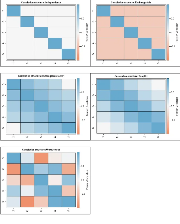
Here we present five basic correlation structures (see Figure 7.1-1 in the appendix for illustration).

Independence

The most basic structure is independence, where each observation within a subject is uncorrelated with another observation. An example of a 4x4 correlation matrix with independence structure is the following

𝑅_𝐼𝑁 = ( 1 0 01 00 00 0 0 00 10 01 ), where 𝐶𝑜𝑟(𝑌_𝑖𝑗, 𝑌_𝑖𝑘) = {1, 𝑖𝑓 𝑗 = 𝑘_{0, 𝑖𝑓 𝑗 ≠ 𝑘} Exchangeable

In exchangeable correlation structure, responses are assumed to be equally correlated within an individual. 𝑅_𝐸𝑋 = ( 1 𝛼 𝛼 1 𝛼𝛼 𝛼𝛼 𝛼 𝛼 𝛼𝛼 𝛼1 𝛼 1 ), where 𝐶𝑜𝑟(𝑌_𝑖𝑗, 𝑌_𝑖𝑘) = {1, 𝑖𝑓 𝑗 = 𝑘_{𝛼, 𝑖𝑓 𝑗 ≠ 𝑘}

(10)

10

Autoregressive AR-1

Two observations closer in time are correlated more than two observations more further in time. This structure is often used in longitudinal designs.Note that 𝑛_𝑖 in this example is 4. 𝑅_𝐴𝑅−1 = ( 1 _𝛼 _𝛼2 _𝛼3 𝛼 𝛼2 𝛼3 1 𝛼 𝛼2 𝛼 1 𝛼 𝛼2 𝛼 1 ), where 𝐶𝑜𝑟(𝑌_𝑖𝑗, 𝑌_{𝑖,𝑗+𝑡}) = 𝛼𝑡, 𝑓𝑜𝑟 𝑡 = 0, . . , 𝑛_𝑖 − 𝑗. Toeplitz

Correlation is the same for any two observations that have the same distance in time. Note that 𝑛_𝑖 in this example is 4.

𝑅𝑇𝑂𝐸𝑃 = ( 1 𝛼₁ 𝛼11 𝛼₂ 𝛼₁ 𝛼𝛼3₂ 𝛼2 𝛼₃ 𝛼𝛼1₂ 𝛼11 𝛼1 1 ), where 𝐶𝑜𝑟(𝑌𝑖𝑗, 𝑌𝑖,𝑗+𝑡) = {_𝛼1, 𝑖𝑓 𝑡 = 0 𝑡, 𝑖𝑓 𝑗 = 1, . . , 𝑛𝑖 − 𝑡 Unstructured

There is no assumption made about any two observations within a subject, so correlation can take a value between -1 and 1. This type of correlation is the most flexible one, but the number of parameters can become too high very quickly.

𝑅𝑈𝑁= ( 1 𝛼₁₂ 𝛼112 𝛼₁₃ 𝛼₂₃ 𝛼𝛼14₂₄ 𝛼₁₃ 𝛼₁₄ 𝛼𝛼23₂₄ 𝛼134 𝛼₃₄ 1 ), where 𝐶𝑜𝑟(𝑌𝑖𝑗, 𝑌𝑖𝑘) = {_𝛼1, 𝑖𝑓 𝑗 = 𝑘 𝑗𝑘, 𝑖𝑓 𝑗 ≠ 𝑘

(11)

11

2.5 Estimation of parameters

The GEE estimator is the solution of the system

∑𝑁𝑖=1𝐷𝑖𝑇𝑉𝑖−1𝑆𝑖 = 0,

where 𝑆_𝑖 = 𝑌_𝑖 − 𝜇_𝑖 with 𝜇_𝑖 = (𝜇_𝑖1, … , 𝜇_𝑖𝑛_𝑖)𝑇 and 𝐷_𝑖 =𝜕𝜇_𝜕𝛽𝑖. Equations reduce to quasi-likelihood equations when there is only one measurement for the outcome variable (𝑛_𝑖 =

1) for each subject. Since estimating equations depend on 𝛽 and correlation parameter 𝛼, and generally have no closed-form solution, solving is based on a two-stage iterative method. (Zeger & Liang 1986)

Parameters of 𝛽 are estimated by solving the equation starting with 𝜙 = 1 and 𝑅_𝑖 as an identity matrix. Estimates are used in calculating fitted values 𝜇̂_𝑖 = 𝑔−1(𝑋_𝑖𝑇𝛽) and residuals 𝑦_𝑖 − 𝜇̂_𝑖. These are used to estimate 𝐴_𝑖, 𝑅_𝑖 and 𝜙. Then these steps are repeated to improve 𝛽̂ until convergence.

One of the properties of GEE estimator is that the estimate of 𝛽 is consistent even when assumed correlation structure among repeated measurements is not correct. That is, 𝛽̂ has the property of being close to the true parameter 𝛽 in large samples. The unbiasedness of the parameter estimates only depends on the correct specification of the model for mean response.

2.6 Sandwich estimator

The following section is based on (Fitzmaurice et al. 2004).

In the GEE context, usual standard errors of 𝛽 are not valid when correlation structure among repeated measurements is misspecified (even though the estimate of 𝛽 is consistent). The variance of the GEE estimator of 𝛽 can be made robust to the misspecification of correlation structure (in a sense that it provides valid standard errors when correlation structure is not correct) by incorporating the empirical variance estimator, called “sandwich” covariance estimator (Diggle et al. 2002). The robustness of sandwich variance estimator is asymptotic meaning that it is a large sample property.

(12)

12

If the sample size is large, the sampling distribution of 𝛽̂ is multivariate normal distribution with mean 𝛽 and covariance in the form of

𝐶𝑜𝑣(𝛽̂) = 𝐵−1_𝑀𝐵−1

where 𝐵−1 = (∑𝑁_𝑖=1𝐷_𝑖𝑇𝑉_𝑖−1𝐷_𝑖)−1 and 𝑀 = ∑𝑁_𝑖=1𝐷_𝑖𝑇𝑉_𝑖−1𝐶𝑜𝑣(𝑌_𝑖)𝑉_𝑖−1𝐷_𝑖. The covariance of 𝛽̂ can be estimated by the “sandwich” estimator

Σ̂_𝑆∶=𝐶𝑜𝑣̂(𝛽̂)=(∑𝑁𝑖=1𝐷̂𝑖𝑇𝑉̂𝑖−1𝐷̂𝑖) −1 ∑𝑖=1𝑁 𝐷̂𝑖𝑇𝑉̂𝑖−1(𝑌𝑖− 𝜇̂_𝑖)(𝑌𝑖− 𝜇 ̂_𝑖)𝑇𝑉̂𝑖−1𝐷̂𝑖(∑𝑁𝑖=1𝐷̂𝑖𝑇𝑉̂𝑖−1𝐷̂𝑖) −1 ,

where 𝛼, 𝜙 and 𝛽 have been replaced by their estimates in 𝐵 and 𝑀, and 𝐶𝑜𝑣(𝑌𝑖) has been replaced with (𝑌_𝑖− 𝜇̂_𝑖)(𝑌_𝑖 − 𝜇̂_𝑖)𝑇 in 𝑀.

The model-based covariance estimator is

𝐶𝑜𝑣̂ (𝛽̂) = 𝐵̂−1_{= (∑} _𝐷_̂ 𝑖𝑇𝑉̂𝑖−1 𝑁 𝑖=1 𝐷̂𝑖) −1

and it yields valid standard errors when the working correlation is correctly specified. The use of sandwich estimator ensures that parameter estimates are consistent even though the working correlation structure may not be correct. However, a correct structure can increase efficiency (Burton et al. 1998). It has been shown that misspecification of the correlation structure can reduce efficiency and inflate variance estimates (Wang & Carey 2003). Therefore, it is important to try to choose the structure which is close to the true correlation matrix 𝑅_𝑖(𝛼). Since one of the aims of fitting a model is to estimate the parameters which describe the correlation structure, one should choose it before the analysis (Burton et al. 1998).

GEE approach assumes data to be missing completely at random (MCAR, (Rubin 1976), (Laird n.d.)), meaning that the missingness does not depend on observed or unobserved responses. If the data are missing at random (MAR), then GEE method can lead to biased results.

(13)

13

2.7 Model inference and interpretation of parameters

Interpretation of regression coefficients depend on the link function used in modelling. Since within-subject correlation is estimated from residuals, parameter estimates are interpreted in a population-average manner. Formal inferences (statistical significance tests) and parameter estimates’ confidence intervals are based upon Wald test. Regression coefficient estimates are divided by their robust (empirical) standard error and the results are treated as Normal standardized deviates (Z statistic). (Burton et al. 1998). It can underperform when sample size is small. Contrasts for a type III test of hypothesis can be tested with generalized score tests.

2.8 Quasi-likelihood Information Criterion (QIC)

Well-known model selection criteria such as Akaike Information Criterion (AIC) or Bayesian Information Criterion (BIC) cannot be applied here since these are likelihood-based and full multivariate likelihood is not used in GEE modelling. However, there is a criterion proposed by (Pan 2001) which is based on AIC but with quasi-likelihood approach, constructed under independence working correlation structure. This quasi-likelihood information criteria (QIC) for GEE models is in the form of

𝑄𝐼𝐶(𝑅) = −2𝑄(𝛽̂(𝑅), 𝐼, ∆) + 𝑡𝑟(Σ̂_{𝑀(𝐼𝑁)}−1 _Σ̂ 𝑆(𝑅)),

where 𝑄(𝛽̂(𝑅), 𝐼, ∆) is the quasi-likelihood under the assumption of working correlation matrix 𝑅, Σ̂_{𝑀(𝐼𝑁)}−1 is the model-based covariance estimator under independence working correlation structure assumption, Σ̂𝑆(𝑅) is the sandwich covariance estimator under the working correlation structure 𝑅 and 𝑡𝑟 is the notation for matrix trace. (Jang 2011) Different models are comparable in the same way as when using AIC – model with smaller QIC value is preferred.

(14)

14

2.9 Summary of GEE

In summary, the GEE approach is a widely used method of estimation in longitudinal designs. Instead of modelling the covariance among repeated measurements, GEE treats it as a nuisance and models the mean response. Covariances and standard errors are valid under the assumption of data missing completely at random.

The GEE has many appealing properties and is often the preferred method for the following reasons. Firstly, even when within-subject correlation structure is not close to the true underlying correlation structure, the GEE estimator 𝛽̂ still gives a consistent estimate. Secondly, the usual standard errors are not valid when correlation structure is misspecified, therefore sandwich estimator of 𝐶𝑜𝑣(𝛽̂) can be used to get valid standard errors. Finally, it is not crucial to assume multivariate normal or any other distribution for the outcome. One needs to specify only the first two moments. The validity of GEE estimates, 𝛽̂, rely only on specifying the correct model for mean response.

(15)

15

3. Using GEE method of estimation in SAS

In this section, two procedures for estimating parameters with GEE in SAS: PROC GENMOD and PROC GLIMMIX are presented. The following chapter is based on SAS User’s Guide(SAS Institute Inc. 2011), where more options are available.

3.1 PROC GENMOD

The GENMOD procedure fits generalized linear models, where it is needed to specify the link function and the probability distribution of the response variable. The following example code will be discussed in detail.

PROCGENMODDATA=data DESCENDING;

CLASS x1(REF='1') id /PARAM=ref;

MODEL y=x1 x2 x1*x2 /LINK=identity DIST=normal TYPE3WALD;

REPEATEDSUBJECT=id /WITHINSUBJECT=timepoints TYPE=ar(1) CORRWCORRB;

RUN;

Note that 𝑦 is the response variable, 𝑥1 and 𝑥2 are the covariates. Each distinct value of the subject-effect (𝑖𝑑) identifies a different subject and each distinct value of the within subject-effect (𝑡𝑖𝑚𝑒𝑝𝑜𝑖𝑛𝑡𝑠) defines a different outcome for the same subject.

PROC GENMOD statement invokes the procedure. DESCENDING option sorts the response variable from highest to lowest (useful with binary and multinomial outcomes). CLASS statement lists all categorical variables and must be before the MODEL statement. PARAM=REF and REF=’level’ need to be specified to be able to use a custom reference level.

MODEL statement specifies the response variable (numeric or character) and covariates (also numeric or character). An intercept is added to the model by default. LINK states the link function and DIST states the probability distribution to be used for 𝑌 in the model. If those are omitted, the model defaults to normal distribution with identity link function. TYPE3 computes generalized score statistics for GEEs and WALD calculates Wald statistics for Type III contrasts (only computed when TYPE3 is specified as well) using empirical (robust) variance estimators.

(16)

16

REPEATED statement invokes the GEE method and specifies the covariance structure of repeated measurements in the model. SUBJECT can be a single effect, interaction or nested and must be listed in the CLASS statement. WITHINSUBJECT defines an effect that specifies an order of repeated measurements. If for example there are some missing values, then specifying WITHINSUBJECT effect, the repeated measurements are ordered in a correct way (missing values are not assumed to be the last measurements). TYPE is used to specify the working correlation matrix. CORRW displays the estimated working correlation matrix and CORRB displays the regression parameter estimates’ correlation matrix (empirical and model-based matrices are presented).

To address the missing completely at random assumption of GEE-type models, the GENMOD procedure can estimate the working correlation by using all available pairs method, and the obtained covariances and standard errors are valid under the MCAR assumption. (SAS User guide). There is an option to use weighted GEE method available in PROC GEE (in SAS version 13) which provides consistent estimates when data are missing at random (MAR)(SAS Institute Inc. 2014).

3.2 PROC GLIMMIX

This procedure can also fit GEE-type models, but there is an additional option to incorporate random effects. An example of GEE approach in the GLIMMIX procedure:

PROCGLIMMIXDATA=data EMPIRICAL;

CLASS x1 id x3;

MODEL y=x1 x2 x1*x2 /LINK=identity DIST=normal SOLUTION;

RANDOM timepoints /SUBJECT=id TYPE=ar(1) RESIDUAL;

RANDOM intercept /SUBJECT=id(x3);

RUN;

PROC GLIMMIX invokes the procedure. The EMPIRICAL option requests the sandwich estimator to be used in calculating covariances for fixed effects.

CLASS statement like in the previous example lists all the categorical variables and must be before the MODEL statement.

MODEL statement names the response variable and covariates. An intercept is added by default. Adding the option SOLUTION produces the scale parameter and parameter estimates for fixed effects.

(17)

17

RANDOM statement invokes the GEE when used with RESIDUAL option. The

𝑡𝑖𝑚𝑒𝑝𝑜𝑖𝑛𝑡𝑠 effect is specified when there’s a need to order the columns of covariance structure by the time variable. SUBJECT option identifies the subjects in the model. All subjects are assumed to be independent from each other. Adding the subject effect nests all the other effects in the RANDOM statement within the subject effect. TYPE specifies the covariance structure in the same way as in the GENMOD procedure.

To incorporate random effects in to the model, one needs to specify it with another RANDOM statement, for example if a variable 𝑥3 is a random effect, specifying

RANDOM intercept /SUBJECT=id(x3);

will treat 𝑥3 as a random effect and assumes subjects are nested within the random effect. Note that with the EMPIRICAL option, adding any random effects requires that data are grouped by subjects.

For the differences between PROC GENMOD and PROC GLIMMIX, refer to appendix 7.2.

(18)

18

4. Analysis of the IndiMed trial

This section will give an overview of IndiMed study design, some descriptive statistics of the data and results of analysis using GEE method of estimation.

4.1 IndiMed study design

The following section is a summary from an article (Meren et al. 2015).

Cardiovascular diseases (CVD) are the number one cause of death in Estonia. One of the risk factors of cardiovascular diseases is an increased arterial blood pressure which is most often caused by hypertension (HT). The incidence rate of HT has been 1400-1500 per 100 000 persons in Estonia from 2010-2013. Incidence of the disease is significantly higher after turning 35 years old and highest in 45-64-year old men.

HT is treatable by medication when good adherence can be achieved. Unfortunately, 25%-60% of HT patients will stop taking medication within the first 6 months of treatment. Low treatment adherence may be caused by disease’s long asymptomatic period, complicated treatment scheme, ignorance of the disease, scepticism of treatment efficacy and high price of medications.

The heritability of cardiovascular disease mortality is estimated to be 38-57%, being different for males and females. Genetic markers tied to risks of CVD have been identified and different risk scores have been calculated using those markers. Results of analysis of the data from the Estonian Genome Center of University of Tartu have been shown that those risk scores are usable in Estonian population. For example, male gene donors in high risk score group have been shown to have 1.9 (95% CL 1.5-2.5) times higher risk for ischemic heart disease than in low risk score group.

It is not known how information about personal genetic risks affect HT patients’ behaviour. The primary objective of IndiMed study is to estimate the effect of personal genetic risk information to patients’ medication adherence and treatment efficiency. The study is based on comparison of two groups – intervention and control. Control group consists of patients who get HT treatment and counselling in the standard way, according to the national guidelines. The intervention group patients get the same treatment as

(19)

19

control group, but additionally they receive information about their genetic risks of four diseases (type 2 diabetes, coronary artery disease, stroke, atrial fibrillation) according to the genetic risk scores. The information is communicated to them by their physician. After treatment start, data on treatment adherence, effectiveness of treatment, body weight and smoking habits are collected from both groups. The difference between systolic and diastolic blood pressure in two groups will be used to draw conclusions about effectiveness of receiving information on genetic risks.

This study is cluster-randomized and there was no blinding of patient and physician. The clusters are physicians who were randomized to intervention and control. Informing patients about their personal risk scores was thought to affect physician’s behaviour towards the patients who did not receive risk score information and therefore decrease the differences of the study groups. For this reason, all of the patients in a physician’s care are in the same study group (intervention or control).

The subjects are 18 to 65-year-old males with 1st or 2nd grade hypertension who did not get medications for HT in the past two months (before entering the study). Duration of patient’s participation in the study is 12 months which includes 5 visits. See appendix 7.3 for the study design figure, including the timeline of the visits and what was measured. Patient’s blood sample was taken during the first visit. From the blood sample, DNA was separated and genotyped in EGCUT lab using real-time PCR method. Using known genetic markers (according to published large-scale Genome-Wide Association Studies, GWAS), personal risk scores were calculated for the following diseases: type 2 diabetes, coronary artery disease, stroke and atrial fibrillation (arrhythmia). For each disease state a patient was classified into one of the two categories: high genetic risk group (highest 10% of risk scores) or an average genetic risk group. The choice of these diseases was motivated by the fact that patients with HT are at high risk for these conditions and also by the existing knowledge on genetic markers affecting the risk.

During the next visits, treatment adherence was evaluated using Morisky Medication Adherence Scale (Morisky et al. 1986) and Brief Medication Questionnaire (Svarstad et al. 1999) allowed to describe the problems encountered while taking medication. Change in arterial systolic blood pressure during the study measured treatment effectiveness. Patient’s health behaviour change was evaluated from body weight and smoking habits

(20)

20

(number of cigarettes per day). The difference in study groups come from visits 2 and 4 where the physician gave information about personal risk scores (intervention group received risk information on 2nd visit and control on 4th visit). The purpose of last (5th) visit was to evaluate long-term changes in patient’s risk behaviours.

4.2 Descriptive statistics

There were 240 patients of whom 127 were in intervention group and 113 were in control group (Table 4.2-1). There were in total 34 doctors of whom 76% had 6 or fewer patients.

Table 4.2-1 Number of patients in intervention and control group.

Group N %

Intervention 127 52.9 Control 113 47.1 Total 240 100.0

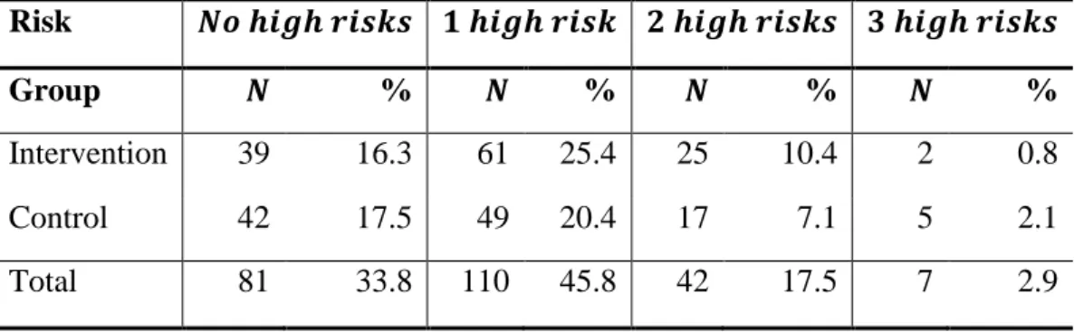
Most of the patients (45.8%) belong to the high risk group for one of the four diseases (Table 4.2-2, note that per cents are based on total 𝑁). On the other hand, nobody had the high risk for all four diseases.

Table 4.2-2 Number of conditions with high genetic risk among subjects by study group.

Risk 𝑵𝒐 𝒉𝒊𝒈𝒉 𝒓𝒊𝒔𝒌𝒔 𝟏 𝒉𝒊𝒈𝒉 𝒓𝒊𝒔𝒌 𝟐 𝒉𝒊𝒈𝒉 𝒓𝒊𝒔𝒌𝒔 𝟑 𝒉𝒊𝒈𝒉 𝒓𝒊𝒔𝒌𝒔

Group 𝑵 % 𝑵 % 𝑵 % 𝑵 %

Intervention 39 16.3 61 25.4 25 10.4 2 0.8

Control 42 17.5 49 20.4 17 7.1 5 2.1

Total 81 33.8 110 45.8 42 17.5 7 2.9

All subjects were between 18 to 65 years old at the time of the first visit with mean weight of 94.3 kilograms, mean height of 179.4 centimeters and mean Body Mass Index (BMI, calculated as 𝐵𝑀𝐼 =_{ℎ𝑒𝑖𝑔ℎ𝑡}𝑤𝑒𝑖𝑔ℎ𝑡₂_/100) of 29.2 (Table 4.2-3Table 4.2-3).

(21)

21

Table 4.2-3 Descriptive statistics for subjects’ age, weight, height and BMI. Age Weight (kg) Height (cm) BMI

N 240 240 239 239 Mean 41.5 94.3 179.4 29.2 Median 42 92 179 28 SD∗ 12.15 17.51 7.70 4.67 Min 18 56 161 20 Max 65 155 202 43

∗_{Standard deviation calculated as}_{𝑆𝐷 = √} 1

𝑁−1∑ (𝑥𝑖− 𝑥̅)2 𝑁

𝑖=1 , where 𝑁 is the number of nonmissing

values of 𝑥.

For blood pressure related studies, risk factors are typically age, BMI and smoking. It is known that regularly smoking increases blood pressure and for this reason smoking is considered as a risk factor. Most of the patients (61.25%) were non-smokers (Table 7.4-1 in the appendix). Blood pressure could be associated with education level, meaning that subjects with higher education level are following the treatment more carefully and therefore have lower blood pressure by the end of the study. Education is also added into the models in the analysis section. Frequencies of patients’ completed education level by study group is displayed in Table 7.4-2 in the appendix.

The following figures (Figure 4.2-1 and Figure 4.2-2) present systolic and diastolic blood pressure box plots by each visit for intervention and control group. In Figure 4.2-1, mean systolic blood pressure in intervention group drops noticeably with three visits. Variability is quite high in both study groups. In Figure 4.2-2, variability and mean diastolic blood pressure in intervention group seem to be a bit smaller than in the control group.

(22)

22

Figure 4.2-1 Box plots of systolic blood pressure by study group and visit. Note that + and Ο inside the boxes display the means and outside the boxes display outliers.

Figure 4.2-2 Box plots of diastolic blood pressure by study group and visit. Note that + and Ο inside the boxes display the means and outside the boxes display outliers.

(23)

23

Response variables, which are systolic and diastolic blood pressures, are assumed to be normally distributed in the population. However, IndiMed data are a sample of subjects with higher blood pressure than in the general population, therefore the distribution is skewed to the right as depicted below.

Figure 4.2-3 Distribution of systolic blood pressure over all visits and subjects. Transforming the response variable may help to fix the skewedness. After log-transformation, systolic blood pressure is approximately normally distributed (Shapiro-Wilk statistic p-value 0.23) as shown in Figure 7.5-1in the appendix.

For diastolic blood pressure (see Figure 7.5-2), neither log or square root transformations were successful according to the Shapiro-Wilk statistic. However, Box-Cox test, which helps to find a power transformation gave log-transformation as the best candidate. Therefore, we will also use log-transformed diastolic blood pressure in analysis (see Figure 7.5-3 for the shape of distribution).

(24)

24

4.3 Analysis

One of the aims of the analysis is to assess the effect of receiving genetic risk information on blood pressure. For this part, intervention and control groups are compared. The hypothesis is that for at least one blood pressure measure (systolic or diastolic), intervention and control groups are statistically different.

Secondly, is there a difference in blood pressure depending on whether the patients who got feedback on genetic risks actually had a high risk for one or more diseases? For this part, intervention group subjects are divided into two groups by the genetic risk: a) no diseases with high genetic risk, b) at least one disease with high genetic risk. The third group will be all patients in the control group. The hypothesis is that there is a difference in mean blood pressure between those three groups.

Since the patients are clustered by doctors, ideally the model should capture a random effect of the doctor, because we want to assume the doctors are randomly chosen from the whole population of doctors. To focus on GEE rather than GEE with additional random effects, the main analysis here will be done assuming a fixed doctor effect by using the GENMOD procedure in SAS. After that, assuming a random doctor effect, the GLIMMIX procedure which allows to add random effects together with GEE, is used. Taking into account the characteristics of the data and how it is collected, AR-1 type of correlation structure between repeated measurements is assumed. Note that other (independent, exchangeable and Toeplitz) correlation structures were tested, but overall AR-1 gave lower QIC.

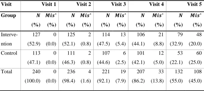
The GEE assumes missing values in data to be missing completely at random. There are many subjects with the last visit information missing at the time of the analysis (Table 7.4-3 in the appendix) and therefore only first four visits are used. The procedure GENMOD assumes MCAR data, but the data are more likely to be missing at random. Therefore, the estimates may be biased.

All models are fit for both systolic and diastolic blood pressures, where these variables are log-transformed beforehand to fix skewedness of the distribution.

(25)

25

Let’s present an example of a log-linear (response is log-transformed and covariates are in the original scale) model’s interpretation of parameter estimates.

Let the model for the blood pressure and estimated parameters be in the form of

𝑙𝑜𝑔(𝐵𝑃) = 4.49 − 0.03 ∙ 𝑔𝑟𝑜𝑢𝑝(𝑖𝑛𝑡𝑒𝑟𝑣𝑒𝑛𝑡𝑖𝑜𝑛) − 0.08 ∙ 𝑣𝑖𝑠𝑖𝑡(2) − 0.10 ∙ 𝑣𝑖𝑠𝑖𝑡(3) − 0.11 ∙ 𝑣𝑖𝑠𝑖𝑡(4)

Then the interpretation of mean blood pressure depends on the reference levels. Here the reference levels are 𝑔𝑟𝑜𝑢𝑝 = 𝑐𝑜𝑛𝑡𝑟𝑜𝑙 and 𝑣𝑖𝑠𝑖𝑡 = 1. The (geometric) mean blood pressure at the reference levels is 𝑒4.49 = 89.12. Mean blood pressure at visit 1 for intervention group is 𝑒(4.49−0.03)= 86.5. The means are different for intervention and control depending on the visits, but the ratio stays the same and is 𝑒𝑒𝑓𝑓𝑒𝑐𝑡 = 𝑒(−0.03)=

0.97. It is convenient to interpret the differences between the two groups in terms of relative change. In this example, switching from control to intervention, the mean blood pressure is expected to decrease by about 3%.

Lastly, we have to consider multiple comparison since we are testing both systolic and diastolic blood pressures. Using Bonferroni correction, the significance level of parameter estimates is at 𝛼 = 0.025 (0.05/2 = 0.025). However, it can be argued that for systolic and diastolic blood pressures this correction is too strict because there is a strong correlation among the response variables (𝐶𝑜𝑟(𝑠𝑦𝑠𝑡𝑜𝑙𝑖𝑐, 𝑑𝑖𝑎𝑠𝑡𝑜𝑙𝑖𝑐) = 0.71).

4.3.1 Intervention vs control group

The following three types of models (of form in section 2.3) for log-transformed systolic and diastolic blood pressures were fitted. Note that group variable is always included in the models, even if nonsignificant, because hypotheses are based on that variable.

1) 𝑙𝑜𝑔(𝑌)~𝑔𝑟𝑜𝑢𝑝

This model compares the overall mean blood pressure (across all visits) of the two study groups. For diastolic blood pressure (DBP), the parameter estimates are in the table below.

(26)

26

Table 4.3-1 Analysis of GEE parameter estimates, diastolic blood pressure, model

𝑙𝑜𝑔(𝑌)~𝑔𝑟𝑜𝑢𝑝.

Response Parameter Estimate SE Z p-value

Diastolic Intercept 4.4890 0.0072 625.89 <.0001 Group (Intervention) -0.0297 0.0094 -3.18 0.0015

According to the analysis, there is a significant difference in control and intervention group (𝑝 = 0.0020, see in Table 7.6-3). The geometric mean of the diastolic blood pressure in the control group is 𝑒4.4890 = 89.03 and for the intervention group it is

𝑒4.4890−0.0297_{= 𝑒}4.4593 _{= 86.43}_{(over all 4 visits). If the patient receives genetic risk} information, we see about 2.9% lower geometric mean of the diastolic blood pressure. For the systolic blood pressure (see Table 7.6-1 and Table 7.6-2), the group variable is nonsignificant at 𝛼 = 0.025 level (𝛽̂ = −0.0136, 𝑝 = 0.0878).

2) 𝑙𝑜𝑔(𝑌)~𝑔𝑟𝑜𝑢𝑝 + 𝑣𝑖𝑠𝑖𝑡 + 𝑑𝑜𝑐𝑡𝑜𝑟

This model assumes the mean blood pressure depends on the groups, visits and doctors. In the model with diastolic blood pressure as response (Table 7.6-6 and Table 7.6-7), the group variable (𝑝 = 0.2694) is nonsignificant. The effect of visit as well as that of the doctor are significant. Compared to visit 1, we see about 8.1% decrease in the geometric mean of diastolic blood pressure in visit 2 and about 10.5% decrease in blood pressure in visit 4.

For systolic blood pressure (Table 7.6-4 and Table 7.6-5), the doctor’s effect (𝑝 =

0.5121) and group’s effect (𝑝 = 0.0559) were nonsignificant.

3) 𝑙𝑜𝑔(𝑌)~𝑔𝑟𝑜𝑢𝑝 + 𝑣𝑖𝑠𝑖𝑡 + 𝑑𝑜𝑐𝑡𝑜𝑟 + 𝐵𝑀𝐼 + 𝑎𝑔𝑒 + 𝑠𝑚𝑜𝑘𝑖𝑛𝑔 + 𝑒𝑑𝑢𝑐𝑎𝑡𝑖𝑜𝑛

This model is similar to the above one, but also including some additional risk factors. These are added to account for the associations which may distort the real relationship between response variable and covariates. When modelling blood pressure, often the risk

(27)

27

factors are BMI and age because higher BMI and older age refer to higher risk of HT. In addition, risk of HT can increase due to smoking. It is possible that patients at higher education level are following the treatment better than patients at lower education level and therefore have lower blood pressure by last visits. For this reason, education level is also included as a covariate.

This model will be fit first by treating doctor as a fixed effect and then treating it as a random effect. Note that the other risk factors are not removed from the model, even if nonsignificant, because we want to control for them.

In the model for diastolic blood pressure (Table 7.6-10 and Table 7.6-11), group is again nonsignificant (𝑝 = 0.2045), therefore there is no evidence for mean blood pressure difference between intervention and control groups. Education is also nonsignificant. BMI, smoking and age all have positive parameter estimates, meaning that high BMI, older age and smoking increase mean blood pressure. For visits the effects are very similar to the previous model 2).

In the random effect model for diastolic blood pressure (Table 7.6-14 and Table 7.6-15), education is nonsignificant as in the above model. However, there is a significant group effect (𝑝 = 0.0024). Parameter estimates for visit are very similar to the fixed effect model.

In systolic blood pressure model (Table 7.6-8 and Table 7.6-9), there is no difference in mean blood pressure between intervention and control. Only visit and BMI are significant with p-values of < 0.0001 and 0.0004 respectively. Visit effects are similar to the above model 2) and higher BMI has a positive parameter estimate which means that higher BMI refers to higher mean blood pressure.

In random effect model for systolic blood pressure (Table 7.6-12 and Table 7.6-13, group is nonsignificant as it is in the fixed effects model. In addition to visit and BMI, education and age are significant variables.

(28)

28

4.3.2 Comparison of intervention group individuals with high genetic risk to individuals at low risk and to the control group

In the next section, mean blood pressure is assessed in subgroups. The following model is fitted:

𝑙𝑜𝑔(𝑌)~𝑠𝑢𝑏𝑔𝑟𝑜𝑢𝑝. The subgroup variable used in the model has a value:

 0, if patient is in control group,

 1, if patient is in intervention group and has no high genetic risks reported,  2, if patient is in intervention group and has high genetic risk for at least one

disease reported.

Table 4.3-2 Subgroup comparison for diastolic blood pressure. Model

𝑙𝑜𝑔(𝑌)~𝑠𝑢𝑏𝑔𝑟𝑜𝑢𝑝.

Diastolic Intercept 4.4890 0.0072 625.81 <.0001 Subgroup (1) -0.0471 0.0117 -4.02 <.0001 Subgroup (2) -0.0217 0.0104 -2.08 0.0371

For diastolic blood pressure (Table 4.3-2 above), subgroup effect is significant (𝑝 =

0.0010, see Table 7.6-17 in the appendix). Compared to control, intervention subgroup 2 does not have statistically different mean diastolic blood pressure. We see about 4.7% decrease in mean blood pressure if the patient receives information on having no high genetic risks for any of the diseases. For subgroup 2, the decrease is about 2.2%. This model has a higher QIC than in model 1) in section 4.3.1 (QICs are 910.8 and 909.1 respectively).

(29)

29

Table 4.3-3 Subgroup comparison for systolic blood pressure. Model

𝑙𝑜𝑔(𝑌)~𝑠𝑢𝑏𝑔𝑟𝑜𝑢𝑝.

Systolic Intercept 4.9561 0.0061 815.90 <.0001 Subgroup (1) -0.0333 0.0102 -3.28 0.0010 Subgroup (2) -0.0044 0.0087 -0.51 0.6109

For systolic blood pressure (Table 4.3-3 above and Table 7.6-16 in the appendix), subgroup effect is significant (𝑝 = 0.0079). The lowest mean systolic blood pressure is (as in the same model with diastolic blood pressure) for patients who received genetic risk information and had no high risks. Compared to control group patients, their mean blood pressure is decreased by about 3.3%. The difference between mean blood pressure between control group and subjects in intervention group who had at least one high disease risk, is nonsignificant. This model also does not have a better fit with the data than model 1) in section 4.3.1 (QIC 908.7 and 907.6 respectively), so it seems that whether or not one receives genetic risk information counts more than what their genetic risks are.

In conclusion for this section, the model which estimates the mean blood pressure for intervention and control group is a better fit to the data than the model where the number of high genetic risks in the intervention group is also taken into account.

(30)

30

4.4 Discussion

The mean blood pressure for intervention and control was not statistically different in most of the fitted models, so it implies that overall, it does not matter whether a patient knows or does not know if they have some high risks for the four diseases (type 2 diabetes, coronary artery disease, stroke and atrial fibrillation). It might be that at first, patients who know their personal risks, are worried and will take medication carefully, but after a while will accept it (or simply do not care) and the effect will fade in time. However, for diastolic blood pressure the effect is significant for model 1 in section 4.3.1. It is intriguing that systolic and diastolic blood pressures seem to respond differently.

Subgroup analysis results indicate that control group (all subjects) and intervention group with at least one high disease risk do not have statistically different mean blood pressures. However, the effect between control and intervention (patients with no high risks) is statistically significant. This is surprising and the reasoning behind that needs further research. It might be that patients who know they have many high disease risks are trying to change their lifestyle and carefully follow medication, but have higher blood pressure for some other reason (for example they are less respondent to treatment or have genetically higher blood pressure). It would also be interesting to know whether mean blood pressures are different for a specific disease risk.

In the near future, when all 5 visits have happened for all patients (at the time of the analysis not all patients had had their last visit), treatment adherence should also be analysed alongside with when and why the subject discontinued the study.

Finally, one should notice that the sample size for this pilot study is rather small. The initial number of patients desired was 300, but only 240 patients joined the study. It is possible that the intervention had an effect, but it was too small to be discovered in this trial. Also the point estimates of the parameters in this study suggest a possibility of a beneficial effect of the intervention. Larger study is necessary to confirm the usefulness of genetic feedback.

(31)

31

5. Conclusion

This thesis gave an overview of Generalized Estimating Equations, which is a method of estimation that accounts for correlations among repeated measurements and is widely used in longitudinal analysis. It has many appealing properties, mainly the robustness to misspecification of correlation structure between the repeated measurements. The validity of GEE parameter estimates and standard errors rely only on specifying the correct model for mean response.

The general guidelines of how to implement GEE-type models was presented in section 3 using SAS procedures PROC GENMOD and PROC GLIMMIX.

The final section implemented GEE-type models on a cluster-randomized study called IndiMed, using data from the Estonian Genome Center of University of Tartu. The clusters are doctors who were randomized to intervention or control group and subjects are men with high blood pressure. All subjects in one cluster are either in intervention (received genetic risk information on the 2nd visit) or control group (received risk information on the 4th visit). Systolic and diastolic blood pressures were compared for the two study groups. Autoregressive AR-1 correlation structure was assumed for the repeated measurements of response variables.

The mean blood pressure was not statistically significant for the two study groups in most of the fitted models which indicates there is no difference if the patient received personal risk information or not. The mean blood pressure was statistically different for patients in control group and patients in intervention group who had no high risks. Control group and intervention group patients with at least one high risk did not have statistically different means for blood pressure. These findings are quite surprising and suggest further analysis should be done. Future research can provide answers to questions whether there are some important factors which determine the blood pressure regarding if patient knows or does not know their risks for diseases.

(32)

32

6. References

Burton, P., Gurrin, L. & Sly, P., 1998. Extending the simple linear regression model to account for correlated responses: an introduction to generalized estimating

equations and multi-level mixed modelling. Statistics in medicine, 17(11), pp.1261–91. Available at: http://www.ncbi.nlm.nih.gov/pubmed/9670414 [Accessed April 9, 2016].

Diggle, P.J. et al., 2002. Analysis of Longitudinal Data Second edi., New York: Oxford University Press.

Fitzmaurice, G.M., Laird, N.M. & Ware, J.H., 2004. Applied Longitudinal Analysis, Hoboken, New Jersey: John Wiley & Sons.

Jang, M.J., 2011. Working correlation selection in generalized estimating equations. University of Iowa. Available at: http://ir.uiowa.edu/etd/2719 [Accessed April 9, 2016].

Laird, N.M., Missing data in longitudinal studies. Statistics in medicine, 7(1-2), pp.305– 15. Available at: http://www.ncbi.nlm.nih.gov/pubmed/3353609 [Accessed May 9, 2016].

Liang, K.-Y. & Zeger, S.L., 1986. Longitudinal Data Analysis Using Generalized Linear Models. Biometrika, 73(1), pp.13–22. Available at:

http://links.jstor.org/sici?sici=0006-3444%28198604%2973%3A1%3C13%3ALDAUGL%3E2.0.CO%3B2-D [Accessed April 9, 2016].

Meren, Ü.H. et al., 2015. The Effect of the Risk Related Personal Genetic Data on Adherence to and Effectiveness of Hypertension Treatment on Estonian Patients: an Overview of the Methodology of the Randomised Study. Eesti Arst, (94), pp.118–122.

Morisky, D.E., Green, L.W. & Levine, D.M., 1986. Concurrent and predictive validity of a self-reported measure of medication adherence. Medical care, 24(1), pp.67– 74. Available at: http://www.ncbi.nlm.nih.gov/pubmed/3945130 [Accessed May 4, 2016].

(33)

33

Pan, W., 2001. Akaike’s Information Criterion in Generalized Estimating Equations. Biometrics, 57(1), pp.120–125. Available at: http://links.jstor.org/sici?sici=0006-341X%28200103%2957%3A1%3C120%3AAICIGE%3E2.0.CO%3B2-Q [Accessed April 29, 2016].

Rubin, D.B., 1976. Inference and Missing Data. Biometrika, 63(3), pp.581–592. SAS Institute Inc., 2014. SAS/STAT® 13.2 User’s Guide, Cary, NC: SAS Institute Inc.

Available at:

http://support.sas.com/documentation/cdl/en/statug/67523/PDF/default/statug.pdf. SAS Institute Inc., 2011. SAS/STAT® 9.3 User’s Guide, Cary, NC: SAS Institute Inc.

Available at:

https://support.sas.com/documentation/cdl/en/statug/63962/PDF/default/statug.pdf. Svarstad, B.L. et al., 1999. The Brief Medication Questionnaire: a tool for screening

patient adherence and barriers to adherence. Patient education and counseling, 37(2), pp.113–24. Available at: http://www.ncbi.nlm.nih.gov/pubmed/14528539 [Accessed May 4, 2016].

Wang, Y.-G. & Carey, V., 2003. Working correlation structure misspecification, estimation and covariate design: Implications for generalised estimating equations performance. Biometrika, 90(1), pp.29–41. Available at:

http://biomet.oupjournals.org/cgi/doi/10.1093/biomet/90.1.29 [Accessed May 9, 2016].

Zeger, S.L. & Liang, K.-Y., 1986. Longitudinal Data Analysis for Discrete and Continuous Outcomes. Biometrics, 42(1), p.121. Available at:

(34)

34

7. Appendix

7.1 Correlation structures

Figure 7.1-1 Examples of Independence, exchangeable, autoregressive(1), Toeplitz and unstructured correlation structures.

(35)

35

7.2 PROC GLIMMIX contrasted with PROC GENMOD

The following is from SAS user guide (SAS Institute Inc. 2011).

SAS procedures GENMOD and GLIMMIX can both fit GEE-type models. However, GENMOD does not allow to add random effects with GEE models (with REPEATED statement).

The GEE estimation in GENMOD procedure uses only R-side covariances whereas GLIMMIX has R-side covariances and also G-side random effects. There is a difference in estimating the covariance parameters: GENMOD estimates these by the method of moments and GLIMMIX by likelihood-based methods.

(36)

36

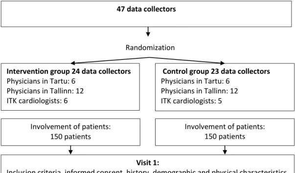
7.3 IndiMed study design and timeline

Figure 7.3-1 Study design, explanations are in text.

47 data collectors

Randomization Intervention group 24 data collectors

Physicians in Tartu: 6 Physicians in Tallinn: 12 ITK cardiologists: 6

Control group 23 data collectors Physicians in Tartu: 6 Physicians in Tallinn: 12 ITK cardiologists: 5 Involvement of patients: 150 patients Involvement of patients: 150 patients Visit 1:

Inclusion criteria, informed consent, history, demographic and physical characteristics, RR, blood sample for DNA, prescription of treatment

Visit 2 (1.5 months after visit 1): Physical characteristics, RR, evaluation of medication compliance, treatment correction if necessary,

explaining DNA test results

Visit 2 (1.5 months after visit 1): Physical characteristics, RR, evaluation of medication compliance, treatment correction if necessary

Visit 3 (3.5 months after visit 1):

Physical characteristics, RR, evaluation of medication compliance, treatment correction if necessary

Visit 4 (6 months after visit 1): Physical characteristics, RR, evaluation of medication compliance, treatment correction if necessary

Visit 4 (6 months after visit 1): Physical characteristics, RR, evaluation of medication compliance, treatment correction if necessary,

explaining DNA test results Visit 5 (12 months after visit 1):

Physical characteristics, RR, evaluation of medication compliance, treatment correction if necessary

(37)

37

7.4 Tables of descriptive statistics

Table 7.4-1 Distribution of patients’ smoking by study group.

Smoking N %

Yes 93 38.75

No 147 61.25

Total 240 100.0

Table 7.4-2 Subjects’ completed level of education by study group. Level of education Primary school Middle school High or vocational school Bachelor’s degree Scientific degree MSc/PhD Missing Group N (%) N (%) N (%) N (%) N (%) N (%) Intervention 2 (0.8) 17 (7.1) 72 (30.0) 29 (12.1) 5 (2.1) 2 (0.8) Control 0 (0.0) 19 (7.9) 62 (25.8) 26 (10.8) 5 (2.1) 1 (0.5) Total 2 (0.8) 36 (15.0) 134 (55.8) 55 (22.9) 10 (4.2) 3 (1.3)

Table 7.4-3 Missing values for blood pressure by visit and study group.

Visit Visit 1 Visit 2 Visit 3 Visit 4 Visit 5

Group 𝑵 (%) 𝑴𝒊𝒔∗ (%) 𝑵 (%) 𝑴𝒊𝒔∗ (%) 𝑵 (%) 𝑴𝒊𝒔∗ (%) 𝑵 (%) 𝑴𝒊𝒔∗ (%) 𝑵 (%) 𝑴𝒊𝒔∗ (%) Interve-ntion 127 (52.9) 0 (0.0) 125 (52.1) 2 (0.8) 114 (47.5) 13 (5.4) 106 (44.1) 21 (8.8) 79 (32.9) 48 (20.0) Control 113 (47.1) 0 (0.0) 111 (46.3) 2 (0.8) 107 (44.6) 6 (2.5) 101 (42.1) 12 (5.0) 53 (22.1) 60 (25.0) Total 240 (100.0) 0 (0.0) 236 (98.4) 4 (1.6) 221 (92.1) 19 (7.9) 207 (86.2) 33 (13.8) 132 (55.0) 108 (45.0) ∗_{Mis: Missing}

(38)

38

7.5 Distribution of systolic and diastolic blood pressures

Figure 7.5-1 Distribution of log-transformed systolic blood pressure over all visits and subjects.

(39)

39

Figure 7.5-3 Distribution of log-transformed diastolic blood pressure over all visits and subjects.

(40)

40

7.6 Tables of analysis results

Model 1. 𝒍𝒐𝒈(𝒀)~𝒈𝒓𝒐𝒖𝒑

Table 7.6-1 Analysis of GEE parameter estimates, systolic blood pressure, model

Systolic Intercept 4.9562 0.0061 816.17 <.0001 Group (Intervention) -0.0136 0.0079 -1.72 0.0859

Table 7.6-2 Score statistics for Type III GEE analysis, systolic blood pressure, model

Response Parameter DF ChiSq p-value Systolic Group 1 2.91 0.0878

Table 7.6-3 Score statistics for Type III GEE analysis, diastolic blood pressure, model

Response Parameter DF ChiSq p-value Diastolic Group 1 9.59 0.0020

(41)

41

Model 2. 𝒍𝒐𝒈(𝒀)~𝒈𝒓𝒐𝒖𝒑 + 𝒗𝒊𝒔𝒊𝒕 + 𝒅𝒐𝒄𝒕𝒐𝒓

𝑙𝑜𝑔(𝑌)~𝑔𝑟𝑜𝑢𝑝 + 𝑣𝑖𝑠𝑖𝑡 + 𝑑𝑜𝑐𝑡𝑜𝑟. Note that rows for doctor are omitted.

Systolic Intercept 5.0336 0.0183 274.71 <.0001 Group (Intervention) 0.0584 0.0106 5.29 <.0001 Visit (2) -0.1024 0.0066 -15.43 <.0001 Visit (3) -0.1228 0.0068 -17.97 <.0001 Visit (4) -0.1201 0.0070 -17.15 <.0001

𝑙𝑜𝑔(𝑌)~𝑔𝑟𝑜𝑢𝑝 + 𝑣𝑖𝑠𝑖𝑡 + 𝑑𝑜𝑐𝑡𝑜𝑟. Response Parameter DF ChiSq p-value

Systolic Group 1 3.65 0.0559

Visit 3 150.64 <.0001 Doctor 33 32.09 0.5121

𝑙𝑜𝑔(𝑌)~𝑔𝑟𝑜𝑢𝑝 + 𝑣𝑖𝑠𝑖𝑡 + 𝑑𝑜𝑐𝑡𝑜𝑟. Note that rows for doctor are omitted.

Response Parameter Estimate SE Z p-value

Diastolic Intercept 4.5724 0.0190 241.22 <.0001 Group (Intervention) -0.0397 0.0315 -1.26 0.2068 Visit (2) -0.0842 0.0062 -13.54 <.0001 Visit (3) -0.1006 0.0069 -14.52 <.0001 Visit (4) -0.1112 0.0071 -15.73 <.0001

(42)

42

𝑙𝑜𝑔(𝑌)~𝑔𝑟𝑜𝑢𝑝 + 𝑣𝑖𝑠𝑖𝑡 + 𝑑𝑜𝑐𝑡𝑜𝑟. Response Parameter DF ChiSq p-value Diastolic Group 1 1.22 0.2694 Visit 3 139.47 <.0001 Doctor 33 66.98 0.0004

(43)

43

Model 3. 𝐥𝐨𝐠 (𝒀)~𝒈𝒓𝒐𝒖𝒑 + 𝒗𝒊𝒔𝒊𝒕 + 𝒅𝒐𝒄𝒕𝒐𝒓 + 𝑩𝑴𝑰 + 𝒂𝒈𝒆 + 𝒔𝒎𝒐𝒌𝒊𝒏𝒈 +

𝒆𝒅𝒖𝒄𝒂𝒕𝒊𝒐𝒏

𝑙𝑜𝑔(𝑌)~𝑔𝑟𝑜𝑢𝑝 + 𝑣𝑖𝑠𝑖𝑡 + 𝑑𝑜𝑐𝑡𝑜𝑟 + 𝐵𝑀𝐼 + 𝑎𝑔𝑒 + 𝑠𝑚𝑜𝑘𝑖𝑛𝑔 + 𝑒𝑑𝑢𝑐𝑎𝑡𝑖𝑜𝑛. Note that rows for doctor are omitted.

Systolic Intercept 4.8569 0.0370 131.15 <.0001 Group (Intervention) 0.0129 0.0248 0.52 0.6020 Visit (2) -0.1018 0.0067 -15.30 <.0001 Visit (3) -0.1211 0.0068 -17.88 <.0001 Visit (4) -0.1196 0.0071 -16.83 <.0001 BMI 0.0035 0.0009 3.84 0.0001 Smoking (yes) 0.0101 0.0084 1.21 0.2269 Education (middle) 0.0163 0.0151 1.08 0.2801 Education (high) -0.0028 0.0096 -0.29 0.7724 Education (BSc) -0.0116 0.0128 -0.90 0.3675 Education (MSc/PhD) -0.0524 0.0205 -2.56 0.0106 Age 0.0008 0.0004 1.96 0.0495

𝑙𝑜𝑔(𝑌)~𝑔𝑟𝑜𝑢𝑝 + 𝑣𝑖𝑠𝑖𝑡 + 𝑑𝑜𝑐𝑡𝑜𝑟 + 𝐵𝑀𝐼 + 𝑎𝑔𝑒 + 𝑠𝑚𝑜𝑘𝑖𝑛𝑔 + 𝑒𝑑𝑢𝑐𝑎𝑡𝑖𝑜𝑛. Response Parameter DF ChiSq p-value

Systolic Group 1 0.23 0.6304 Visit 3 147.53 <.0001 BMI 1 12.59 0.0004 Smoking 1 1.45 0.2291 Doctor 33 26.33 0.7881 Education 4 7.80 0.0991 Age 1 3.78 0.0517

(44)

44

𝑙𝑜𝑔(𝑌)~𝑔𝑟𝑜𝑢𝑝 + 𝑣𝑖𝑠𝑖𝑡 + 𝑑𝑜𝑐𝑡𝑜𝑟 + 𝐵𝑀𝐼 + 𝑎𝑔𝑒 + 𝑠𝑚𝑜𝑘𝑖𝑛𝑔 + 𝑒𝑑𝑢𝑐𝑎𝑡𝑖𝑜𝑛. Note that rows for doctor are omitted.

Diastolic Intercept 4.4737 0.0526 84.98 <.0001 Group (Intervention) -0.0608 0.0435 -1.40 0.1625 Visit (2) -0.0845 0.0063 -13.45 <.0001 Visit (3) -0.1004 0.0070 -14.27 <.0001 Visit (4) -0.1109 0.0072 -15.46 <.0001 BMI 0.0032 0.0011 2.86 0.0042 Smoking (yes) 0.0196 0.0084 2.33 0.0196 Education (middle) -0.0299 0.0333 -0.90 0.3696 Education (high) -0.0234 0.0320 -0.73 0.4641 Education (BSc) -0.0309 0.0327 -0.94 0.3457 Education (MSc/PhD) -0.0313 0.0374 -0.84 0.4031 Age 0.0008 0.0004 2.34 0.0194

𝑙𝑜𝑔(𝑌)~𝑔𝑟𝑜𝑢𝑝 + 𝑣𝑖𝑠𝑖𝑡 + 𝑑𝑜𝑐𝑡𝑜𝑟 + 𝐵𝑀𝐼 + 𝑎𝑔𝑒 + 𝑠𝑚𝑜𝑘𝑖𝑛𝑔 + 𝑒𝑑𝑢𝑐𝑎𝑡𝑖𝑜𝑛. Response Parameter DF ChiSq p-value

Diastolic Group 1 1.61 0.2045 Visit 3 136.02 <.0001 Doctor 33 55.61 0.0082 BMI 1 7.15 0.0075 Smoking 1 5.24 0.0220 Education 4 1.45 0.8355 Age 1 5.14 0.0234

Generalized Estimating Equations: an overview and application in IndiMed study

Maia Arge

Generalized Estimating Equations: an overview and

application in IndiMed study

Mathematical statistics

Master’s thesis (30 EAP)

Table of contents

1.

Introduction

2.

Generalized Estimating Equations (GEE)

2.1

Introduction to Generalized Estimating Equations

2.2

Quasi-likelihood estimator

2.3

Marginal models

2.4

Correlation structures

2.5

Estimation of parameters

2.6

Sandwich estimator

2.7

Model inference and interpretation of parameters

2.8

Quasi-likelihood Information Criterion (QIC)

2.9

Summary of GEE

3.

Using GEE method of estimation in SAS

3.1

PROC GENMOD

3.2

PROC GLIMMIX

4.

Analysis of the IndiMed trial

4.1

IndiMed study design

4.2

Descriptive statistics

4.3

Analysis

4.4

Discussion

5.

Conclusion

6.

References

7.

Appendix

7.1

Correlation structures

7.2

PROC GLIMMIX contrasted with PROC GENMOD

7.3

IndiMed study design and timeline

7.4

Tables of descriptive statistics

7.5

Distribution of systolic and diastolic blood pressures

7.6

Tables of analysis results