International High Performance Buildings
Conference
School of Mechanical Engineering
2014
Improving HVAC Performance Through
Spatiotemporal Analysis of Building Thermal
Behavior
Michael Vincent Georgescu
University of California, Santa Barbara, United States of America, [email protected]
Igor Mezic
University of California, Santa Barbara, United States of America, [email protected]
Follow this and additional works at:
http://docs.lib.purdue.edu/ihpbc
This document has been made available through Purdue e-Pubs, a service of the Purdue University Libraries. Please contact [email protected] for additional information.
Complete proceedings may be acquired in print and on CD-ROM directly from the Ray W. Herrick Laboratories athttps://engineering.purdue.edu/ Herrick/Events/orderlit.html
Georgescu, Michael Vincent and Mezic, Igor, "Improving HVAC Performance Through Spatiotemporal Analysis of Building Thermal Behavior" (2014).International High Performance Buildings Conference.Paper 154.
Improving HVAC Performance Through Koopman Mode Analysis of Building
Data
Michael Georgescu
1*, Igor Mezic
21
Department of Mechanical Engineering
University of California, Santa Barbara
Santa Barbara, California, USA
email: [email protected]
2
Department of Mechanical Engineering
University of California, Santa Barbara
Santa Barbara, California, USA
email: [email protected]
* Corresponding Author
ABSTRACT
In this work, an energy audit case study of a LEED silver university building is performed by decomposing building data into spatial-temporal modes known as Koopman modes. Koopman modes are influenced by heat loads, from internal and external sources, that a building is subject to, and analysis of these modes provides greater understanding of a building's thermal behavior. In the presented application of this framework, examples of energy waste are identified including faulty equipment operation, unnecessary equipment usage, and HVAC operating conditions requiring high energy to maintain. Through addressing the issues discovered, energy usage of the case study building is reduced by 13% with no side effects seen in building comfort. Koopman mode analysis has previously been used to study the thermal behavior of building models, but has seen only limited implementation using actual building data.
1. INTRODUCTION
Commercial buildings have a significant impact on energy use as they account for 18% of the total primary energy consumption in the United States DOE (2008). As this percentage rises from the construction of new buildings, energy efficiency is becoming increasingly emphasized in all stages of the building life cycle. Despite the efforts of designers and owners to increase energy efficiency, many cases of underachievement are documented for both new and existing buildings.
Examples of buildings performing below expectations can be seen in the works Torcellini et al. (2006) and Copeland (2012) although numerous examples exist throughout building literature. From these works, and others, it would seem that building underperformance is not limited to new or existing buildings, and that even buildings designed with energy efficiency in consideration routinely fail to meet performance goals. In the case studies mentioned, a common reason for inefficiencies is insufficient monitoring during building management where equipment is not maintained properly or is operated differently from the original design intent. Because space heating and cooling accounts for approximatley 40% of commercial building energy consumption DOE (2008), and HVAC operational faults from insufficient monitoring can lower system efficiency by 20% Wiggins and Brodrick (2012), the increase in energy consumption due to faulty operation can be considerable. In Energy Center of Wisconsin (1998), it is estimated that up to 80 percent of buildings have inefficiency problems.
To help resolve these issues, improvements are needed in building monitoring, but a typical building, with a modern building management system, produces between several thousand and million data points per day depending on the level of instrumentation. On the other hand, a building operator usually has few key questions that they would like answered from this data; is the building comfortable, functioning normally, and is energy wasted in the operation of the building? In a scenario where a building operator is managing multiple buildings, these questions can remain
unanswered unless a major problem is encountered. Tools are necessary to quickly and easily aggregate data from building management systems to help answer these questions.
Within literature, research exists on advanced monitoring techniques and sensor data aggregation. In Meyers et al. (1996), several visualization techniques are demonstrated where data is visualized in three-dimensional carpet-plot images which show the evolution of a building sensor measurement over a year long time scale. A similar approach is used in Raftery and Keane (2011) where contour plots are used to compare a statistic to two uncorrelated axes (e.g. hour of day and day of week) emphasizing the effect of external influences (such as occupancy) to a measurement (temperature, energy consumption, etc...). Other works exist on transformations performed on data to extract features which are useful for building HVAC fault detection and diagnostics (See House et al. (2001); Schein et al. (2006) and references).
In this work, the thermal behavior rooms are monitored using an approach based on the Koopman operator and the concept of Koopman modes: the Koopman operator is an infinite-dimensional, linear operator that captures nonlinear, finite-dimensional dynamics. Using properties of the operator, building data can be decomposed into spatial-temporal modes revealing features of the data which occur at different time scales. When this approach is applied using room level building data (e.g room temperatures), Koopman modes can be visualized on a plan view of a building allowing the data to be represented spatially. Visualizing these modes allows a practitioner to quickly inspect the behavior of rooms and HVAC components and determine if they are operating correctly. Using this technique, forms of energy waste can be identified including faulty equipment operation, unnecessary equipment usage, and HVAC operating conditions requiring high energy to maintain.
The notion of Koopman modes was first introduced in Mezic (2005) and later applied in the study of fluid dynamics Rowley et al. (2009) and power grid instabilities Susuki and Mezic (2010). The Koopman operator approach has also previously been used to study the thermal behavior buildings; in Eisenhower et al. (2010), an EnergyPlus model of a building was partially calibrated to measured data by comparing the modes produced by the model to that from measured space temperature data, and in Georgescu et al. (2012), Koopman modes are used to validate modeling practices used in the ASHRAE 90.1 modeling appendix ASHRAE (2010). This paper is based on the analysis of Eisenhower et al. (2010) where Koopman modes are calculated from measurements of room temperature. This paper extends the previous analysis to the study of Koopman modes calculated from measurements of HVAC quantities (ex. flows, discharge / supply temperature, ...).
The remainder of this paper is organized as follows: in the next section, an overview of the Koopman operator is given. Then in section 3, the case study building is introduced. In section 4, Koopman modes of a building data are calculated and analyzed. The paper is concluded with a discussion of the achieved energy savings and directions for future research.
2. THE KOOPMAN OPERATOR
In the analysis of dynamical systems, understanding the structure of systems plays a considerable role. Because the equations describing a system, such as that of a building heat transfer and energy consumption, can be of a high dimension and incapable of being expressed analytically, methods are required which are measurement, or data-based, to study such systems. In this context, properties of the Koopman operator are applicable, and can be applied to buildings for the analysis and visualization of these systems. By projecting the time-evolution of sensor measurements onto eigenfunctions of the operator, spatial features of a system being studied can be extracted.
To introduce the Koopman operator, consider the evolution of a nonlinear dynamical system given by
x(t+1)=F(x(t)) (1)
wherex∈Mare the state space variables belonging to a finite, but multi-dimensional spaceM, andF∶M→Mmaps the variables at timetto timet+1. The Koopman operatorUis a linear operator that acts onMin the following manner: forg∶M→R, wheregis a function describing observations of the state space variables,Umapsgto a new function
Ug(x)=g(F(x(t)))=g(x(t+1)). (2) Although the dynamical system may be nonlinear and evolve on a finite-dimensional space, the Koopman operator is linear, but infinite-dimensional.
The Koopman operator describes the evolution of an observable one step in time, and iterative application of the operator describes the trajectory of the observable. Because the Koopman operator is linear, its eigenfunctions and eigenvalues are defined as follows: for eigenfunctionψk∶M→Cand constant eigenvaluesλk∈C
Uψk(x)=λkψk(x). k=1,2, ... (3) Observables can be expressed as projections onto the eigenfunctions of the Koopman operator by
g(x)=
∞
∑
k=1
λkψk(x)vk. (4)
In the analysis of building data, observables are often vector valued (e.g. temperature of multiple rooms). When this is the case, vector-valued observables,G∶M→Rm, can similarly be expressed by
G(x)= ⎡⎢ ⎢⎢ ⎢⎢ ⎣ g(x)1 ... g(x)n ⎤⎥ ⎥⎥ ⎥⎥ ⎦ (5)
In Eq.4,{vk}∞k=1 are a set of vectors called Koopman modes, and are coefficients of the projections of observables onto the eigenfunctions of the operator. Koopman modes describe the dynamics of observables at different frequencies (proportional toλk), and will be the basis for the analysis of building data described later in this paper.
We assumeg(x)is in the span of eigenfunctions. When this is the case, Koopman modes ofg(x)can be computed by calculating Fourier averages,g∗ω(x)∈C, of the form:
g∗ω(x)= lim n→∞ 1 n n−1 ∑ j=0 ei2πjωg(x(j)). (6)
Ifg∗ωis nonzero, the observable,g(x), has a nonzero component within a Koopman mode of frequencyω. The notion of Koopman modes was introduced in Mezic (2005), and this relationship between Fourier analysis and Koopman modes is first identified. There are several methods available for calculating Koopman modes such as using the Arnoldi algorithm Susuki and Mezic (2010), or by using Fourier averages of the spatial field Mezic (2005). When observables are periodic, the decomposition can be computed using discrete Fourier transformation Rowley et al. (2009). For more information about data decompositions using the Koopman operator, refer to the references above and review paper of Budisic et al. (2012).
3. CASE STUDY BUILDING
The Student Resources Building (SRB) was constructed in 2007 at the University of California, Santa Barbara. The building is a hub for campus organizations and student services.
The 68,000 sqft. floor plan contains three above ground floors and is separated into northern and southern halves by a 4 story 5500 sqft. atrium acting as a divider between these halves. The building includes several areas of different
Figure 1:(Color Online) Exterior views of the university building studied. Northern entrance of the SRB (left), and southern entrance (right).
space utilization including offices, classrooms, child daycare, and auditorium / theater, as well as common areas were student groups can assemble.
Energy saving features of the building design include extensive use of natural ventilation throughout the building floor space. The atrium and offices in the perimeter of the building are naturally ventilated with baseboard heaters while rooms in the core of the buildings are conditioned by one of six air handling units. Mechanically ventilated rooms are conditioned by either variable air volume units with terminal reheat or constant air volume units. Fan coil units condition unoccupied rooms that contain electrical or telecommunications equipment which require continuous space cooling. HVAC chilled water is provided by district cooling from a campus chilled water loop while heating for hot water is generated by a gas fired boiler located in the plant of the building.
Because of the coastal setting, cool offshore winds flow perpendicular to the length of the atrium. Using motors along the perimeter of the atrium, vents can be opened allowing hot air to advect from the atrium ceiling while cool outdoor air is drawn through vents located on the ground floor of the building.
3.1 DATA COLLECTION
For the building studied, data was collected from an SQL server containing archived building management system (BMS) data. From the BMS, measurements of space temperature, HVAC equipment temperatures (i.e. discharge and supply), and HVAC equipment flows were collected. Because some areas of the building are normally unoccupied (e.g. the building plant, closets, etc...) certain rooms are not measured by the BMS.
4. KOOPMAN MODE ANALYSIS OF THE SRB
Koopman modes can be calculated from spatially distributed measurements such as space temperature, discharge air temperature or flows (of HVAC end-devices), and can be used to analyze spatial-temporal features of a building's thermal response. Because Koopman modes are defined on the complex set of numbers, each mode has an associated amplitude and phase. The amplitude and phase of Koopman modes are related to measured quantities by:
xm(t)=
∞
∑
k=1
∥Vk,m∥sin(ωkt+ ∠Vk,m), (7)
whereωkis the frequency corresponding to the k-th Koopman mode.
The magnitude and phase of Koopman modes calculated from building data are a result of oscillatory inputs (energy demands such as plug loads, lighting, HVAC, etc...) that the building is subject to. The calculated Koopman modes
Figure 2:Visualizations of building data using the Koopman operator method: Koopman spectrum (section A), Koop-man mode magnitude (section B), and KoopKoop-man mode phase (section C). Temperature measurements of rooms circled in red and blue in the magnitude and phase plot are shown in Section D highlighting how features of a time-series are captured by Koopman modes.
capture these effects and represent the impact of these inputs on the dynamics of building energy consumption at various time-scales.
Figure 2 is an example of the various ways that building data can be represented in this framework. In section A, the spectrum of the Koopman operator calculated from measurements of room temperature is shown. Each column of the spectrum corresponds to a Koopman mode at a particular frequency and each row represents the temperature response of a room. Horizontal bands in the spectrum signify that the temperature behavior of a particular room has spectral content across multiple Koopman modes while vertical bands indicate that a large group of rooms behave collectively at a time scale such that their response is captured by a Koopman mode of appropriate frequency. Because building data contains many periodicities, the Koopman operator approach effectively captures these patterns. For example, the magnitude and phase of the 24 hour Koopman mode are shown in sections B and C. This mode is the largest in magnitude within the spectrum, and it reflects the overall temperature behavior of rooms within the building at the daily time scale. When visualized against a plan view of the building, features of the temperatures response of rooms can quickly be interpreted keeping in mind the relationship between Koopman mode magnitude and phase to time-series measurements in equation 7. As an example, two rooms with a difference in magnitude and phase are circled, with their respective time series shown in section D. The room circled in blue has a larger Koopman mode magnitude (larger daily temperature oscillations) and a Koopman mode phase corresponding to peak temperature occurring at about 6PM while the room circle in red has a smaller Koopman mode magnitude and a Koopman mode phase corresponding to
Figure 3:Koopman spectrum (top) calculated from measurements of VAV discharge air temperature. Within the spec-trum, the response of two VAVs are circled which exhibit unstable oscillatory behavior. The time-series measurements of these two VAVs are shown on bottom.
peak temperature occurring at about 6AM. Through visualization of the spectrum of the Koopman operator and the magnitude and phase of Koopman modes, a practitioner can quickly examine the behavior of different sets of building sensors to determine building comfort or detect faulty behavior. Examples of different types of inefficient building behavior identified with this approach on the case study building will now be discussed.
4.1 IDENTIFIED INEFFICIENCIES
Using the framework of analyzing the Koopman spectrum and Koopman modes, several building faults occurring at the room and VAV level can be identified can be identified. For the analysis in this section, Kooman modes were calculated from the discharge air temperature of VAVs as they correspond to the control action of a VAV controller. The following are examples of two types of commonly discovered issues.
Figure 4: 24 hour Koopman mode phase (top) calculated from measurements of VAV discharge air temperature. Circled rooms denote an area where adjacent VAVs have a phase difference ofπ. This phase difference corresponds competing VAVs exhibiting opposite control action. Time-series measurements of these two VAVs are shown below where one VAV is continuously cooling and the other is continuously heating.
VAV Behavior Tuning: As a first example, we investigate data corresponding to VAV discharge air temperature (DAT) and notice that in the Koopman spectrum , shown in Figure 3, two rooms have spectral content across multiple Koopman
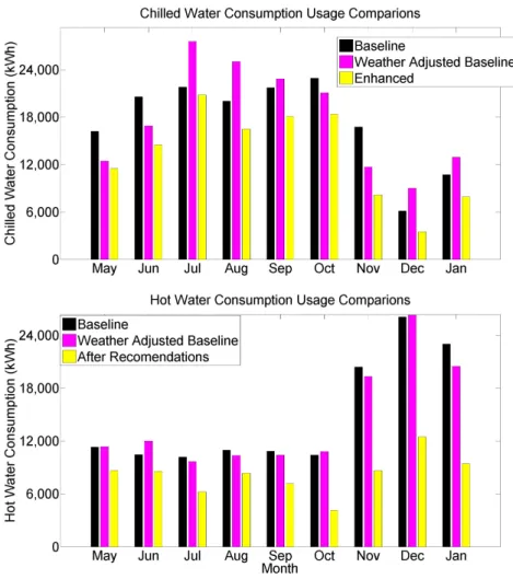
Figure 5:Comparison of chilled water and natural gas consumption before and after building operational changes are made. Models based on degree day methodology illustrate that savings are not due to differences in weather in the time periods considered.
modes. The appearance of horizontal bands in the spectrum corresponds to oscillatory DAT behavior and is generally undesirable in control loops since it produces instability. The time series in the bottom of Figure 3 confirms this observation as the measured DAT of two VAVs shown quickly oscillate between heating and cooling multiple times a day. As it turns out, this issue was caused by a narrow deadband temperature set-point in each VAV's control loop causing the action of each controller to alternate between heating and cooling.
Simultaneous Heating and Cooling: In a second example, we again investigate the behavior of VAV DAT by looking at the 24 hour Koopman mode phase. When VAV DAT is examined, the 24 hour Koopman mode phase, shown in Figure 4, relates to the ratio of heating to cooling that a VAV provides to a room. Rooms with a phase of±πare continuously heating while rooms with a phase of 0 are continuously cooling. Rooms with a intermediate phase experience some combination of heating and cooling within the daily time scale. Circled in the Figure 4 are several rooms which are adjacent but have a difference in phase ofπ. Because many of these rooms are connected by breezeways, this corresponds to simultaneous heating and cooling of adjacent rooms which can cause significant energy waste. This type of issue was found to be caused by large differences in the temperature set-point of the adjacent rooms. For the areas circled, rooms with a phase of 0 had a temperature set-point of 74○F while rooms with a phase of±π had a temperature set-point of 68○F.
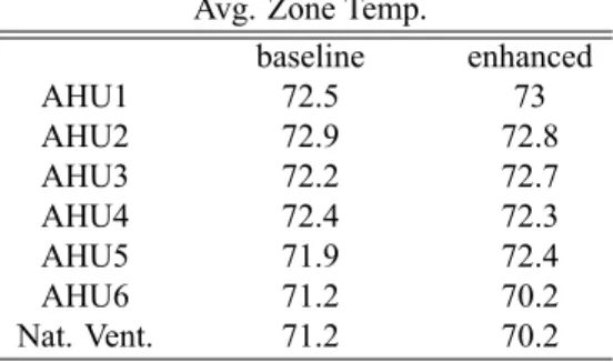
Table 1:Change in average room temperature (during occupied hours) before and after implementation of performance measures.
Avg. Zone Temp.
baseline enhanced AHU1 72.5 73 AHU2 72.9 72.8 AHU3 72.2 72.7 AHU4 72.4 72.3 AHU5 71.9 72.4 AHU6 71.2 70.2 Nat. Vent. 71.2 70.2
5. RESULTS
Thus far, features of the Koopman operator spectrum and Koopman modes have been connected to characteristics of time series data. This approach was applied to study building data and identify instances of inefficient HVAC operation. Through the use of Koopman mode analysis, features of the thermal behavior of the building were visualized and several types of VAV faults were identified. From this study, building data from the SRB was analyzed over a 9 month period from May 2010 - February 2011. During the time-period, the discussed HVAC faults were documented, and measures were implemented to resolve them. Solutions took the form of set-point adjustments of HVAC components to eliminate simultaneous heating, controller oscillations, and increase/maintain comfort in areas of the building through adjustment of HVAC schedules.
From the information gathered, overnight boiler usage was eliminated as it was observed that baseboard heating was not utilized. Because baseboard heating is not measured, this conclusion was made from analysis of Koopman modes of room temperature in naturally ventilated spaces. Also, AHU supply air temperature was increased from 55 degrees to 60 degrees to make greater usage of AHU economizers. Based on the usage of VAV reheat and temperature of adjacent naturally ventilated rooms, it was believed that this change would not adversely affect building comfort. Individual rooms, and pairs of rooms, exhibiting controller issues (simultaneous heating and cooling, or oscillatory behavior) had their thermostat set-points changed to eliminate the issues.
To quantify energy savings, building energy consumption was compared from the baseline nine month period (May 2010 - February 2011) to the same time-period one year later after all savings measures had been enacted. Using re-gression analysis based on the cooling degree day and heating degree day methodology, statistical models were created, correlating building energy consumption to outdoor air temperature, to account for changes in environmental condi-tions between the time periods considered. The comparison of actual building energy consumption as well as predicted consumption from the normalized regression models are shown in Figure 5. Savings were determined by comparing the period of enhanced building performance (May 2011 - February 2012) to the baseline (May 2010 - February 2011) in conjunction with predictions produced by the regression models. In this comparison, energy consumption in the enhanced operation scenario was considerably less then the baseline. Between the two time periods which were mon-itored, consumption of chilled water (HVAC cooling) and natural gas (HVAC heating) decreased by 25% and 44 % respectively. Because the amount of electric consumption due to HVAC loads is small compared to the total electric consumption of the building, no changes in electrical consumption were measured. From the measures enacted, the total energy consumption of the building reduced by 13% while weather normalized models reveal similar reductions and show that the energy savings are not due to changes in weather between the two time periods considered. Because measures consisted of changing room temperature set-points and HVAC schedules of operation, one expecta-tion would be to see a decrease in the comfort of building spaces. Although a full analysis of the changes in comfort is outside the scope of this paper, Table 1 compares the average measured temperature of rooms between the time periods monitored. For all air handling units and naturally ventilated rooms, the changes in average temperature was within a 1○F during periods of building occupancy. Although a comparison of average temperature is a simplified approach, major improvements in comfort were noticed through elimination of space overheating. Also, occupant complaints of discomfort reduced lending to the belief that the measures had no negative effect on comfort.
6. CONCLUSIONS
In this paper, an energy audit of a university building was carried out and based on examining Koopman modes calcu-lated from building data. Koopman mode analysis of building temperature data revealed VAV discharge temperatures uncovered issues such as simultaneous heating and cooling of adjacent building spaces, and controller instabilities caus-ing high frequency oscillations of space temperatures. Additionally, Koopman mode analysis of space temperatures provided information on the whole-building temperature behavior of the SRB and provided confidence that relaxing set-points and schedules would not adversely affect comfort.
From the analysis and measured enacted, the net building energy consumption was reduced by 13% which have been shown to not be a result of changes in weather from the time periods considered. This was accomplished without any noticeable changes to building comfort. The focus of this paper is to demonstrate Koopman mode analysis on building management system data, and to connect characteristics of the observed Koopman modes to features of the temper-ature behavior of building spaces and HVAC components. Future work will be in extending this approach through a quantitative evaluation of Koopman modes. With this, potential applications of Koopman mode analysis include fault detection and integration into building energy management systems for advanced energy monitoring.
NOMENCLATURE
F nonlinear functionx state space variables
xi i-th state space variable
M high dimension manifold
R set of real numbers
U Koopman operator
g observation function
G vector-valued observation function (G=(g1, ...,gm)T)
ψk k-th Koopman eigenfunction
λk k-th Koopman eigenvalue
vk k-th Koopman mode of observable
Vk k-th Koopman mode of vector-valued observable (Vk(G)=(vk,1, ...,vk,m)T)
k eigenvalue/eigenfunction index
C set of complex number
REFERENCES
(2008). Building energy data book. U.S. Department of Energy.
ASHRAE (2010). ASHRAE Standard 90.1:Energy Standard for Buildings Except Low-Rise Residential Build-ings.https://www.ashrae.org/standards-research--technology/standards--guidelinesAccessed: 7/15/2013.
Budisic, M., Mohr, R., and Mezic, I. (2012). Applied koopmanism.Chaos: An Interdisciplinary Journal of Nonlinear Science, 22(4):047510.
Copeland, C. C. (2012). Improving energy performance of nyc's existing office buildings. ASHRAE Journal, pages 28--38.
Eisenhower, B., Maile, T., Fischer, M., and Mezic, I. (2010). Decomposing buildig system data for model validation and analysis using the koopman operator. InBuilding Simulation, 2010. Proceedings. Fourth National Conference
of the International Building Performance Simulation Association, pages 434 --441.
Energy Center of Wisconsin (1998).Building Commissioning: Survey of Attitudes and Practices in Wisconsin. Energy Center of Wisconsin.
Georgescu, M., Eisenhower, B., and Mezić, I. (2012). Creating zoning approximations to building energy models using the koopman operator. InSimBuild 2010. Proceedings. Fifth National Conference of International Building
Per-formance Simulation Association-USA, pages 40 -- 47. http://www.ibpsa.us/simbuild2012/Papers/SB12_
TS01b_3_Georgescu.pdfAccessed: 7/15/2013.
House, J. M., Vaezi-Nejad, H., and Whitcomb, J. M. (2001). An expert rule set for fault detection in air-handling units.
Transactions-American Society of Heating Refrigerating and Air Conditioning Engineers, 107(1):858--874.
Meyers, S., Mills, E., Chen, A., and Demsetz, L. (1996). Building data visualization for diagnostics.ASHRAE journal, 38(6):8.
Mezic, I. (2005). Spectral properties of dynamical systems, model reduction and decompositions.Nonlinear Dynamics, 41:309--325.
Raftery, P. and Keane, M. (2011). Visualizing patterns in building performance data. In12th Conference of International
Building Performance Simulation Association, Sydney.
Rowley, C., Mezic, I., Bagheri, S., Schlatter, P., and Henningson, D. (2009). Spectral analysis of nonlinear flows.
Journal of Fluid Mechanics, 641:115--127.
Schein, J., Bushby, S. T., Castro, N. S., and House, J. M. (2006). A rule-based fault detection method for air handling units.Energy and Buildings, 38(12):1485--1492.
Susuki, Y. and Mezic, I. (2010). Nonlinear koopman modes of coupled swing dynamics and coherency identification.
InPower and Energy Society General Meeting, 2010 IEEE, pages 1 --8.
Torcellini, P. A., Pless, S., Deru, M., Griffith, B., Long, N., and Judkoff, R. (2006).Lessons learned from case studies
of six high-performance buildings. National Renewable Energy Laboratory.
Wiggins, M. and Brodrick, J. (2012). Hvac fault detection. ASHRAE Journal, pages 78--80.
ACKNOWLEDGMENTS
The authors would like to acknowledge Valerie Eacret and Erika Eskenazi for their contributions, as well as Kazimir Gasljevic and UC Santa Barbara Facilities Management. This work was partially funded by Army Research Office Grant W911NF-11-1-0511, with Program Manager Dr. Sam Stanton.