University of Wollongong University of Wollongong
Research Online
Research Online
Centre for Statistical & Survey Methodology
Working Paper Series Faculty of Engineering and Information Sciences 2011
Evaluating the volatility forecasting performance of best fitting GARCH
Evaluating the volatility forecasting performance of best fitting GARCH
models in emerging asian stock markets
models in emerging asian stock markets
Chaiwat KosapattarapimUniversity of Wollongong, [email protected] Yan-Xia Lin
University of Wollongong, [email protected] Michael McCrae
University of Wollongong, [email protected]
Follow this and additional works at: https://ro.uow.edu.au/cssmwp
Recommended Citation Recommended Citation
Kosapattarapim, Chaiwat; Lin, Yan-Xia; and McCrae, Michael, Evaluating the volatility forecasting performance of best fitting GARCH models in emerging asian stock markets, Centre for Statistical and Survey Methodology, University of Wollongong, Working Paper 13-11, 2011.
https://ro.uow.edu.au/cssmwp/87
Research Online is the open access institutional repository for the University of Wollongong. For further information contact the UOW Library: [email protected]
Copyright © 2008 by the Centre for Statistical & Survey Methodology, UOW. Work in progress, no part of this paper may be reproduced without permission from the Centre.
Centre for Statistical & Survey Methodology, University of Wollongong, Wollongong NSW
Centre for Statistical and Survey Methodology
The University of Wollongong
Working Paper
13-11
Evaluating the Volatility Forecasting Performance of Best Fitting
GARCH Models in Emerging Asian Stock Markets
Evaluating the Volatility Forecasting Performance of Best
Fitting GARCH Models in Emerging Asian Stock Markets
Chaiwat Kosapattarapim1 Yan-Xia Lin2 Michael McCrae3
Center for Statistical and Survey Methodology
School of Mathematics and Applied Statistics , University of Wollongong Wollongong, NSW 2522, AUSTRALIA
Abstract
Problem statement : While modeling the volatility of returns is essential for many
areas of finance, it is well known that financial return series exhibit many non-normal characteristics that cannot be captured by the standard GARCH model with a normal error distribution. But which GARCH model and which error distribution to use is still open to question, especially where the model that best fits the in-sample data may not give the most effective out-of-sample volatility forecasting ability which we use as the criterion for the selection of the most effective model from among the alternatives. Approach:
In this study, six simulated studies in GARCH (p,q) with six different error distributions (normal, skewed normal, student-t, skewed student-t, generalized error distribution and skewed generalized error distribution) are carried out. In each case, we determine the best fitting GARCH model based on the AIC criterion and then evaluate its out- of-sample volatility forecasting performance against that of other models. The analysis is then carried out using the daily closing price data from Thailand (SET), Malaysia (KLCI) and Singapore (STI) stock exchanges. Results : Our simulations show that although the best fitting model does not always provide the best future volatility estimates the differences are so insignificant that the estimates of the best fitting model can be used with confidence. The empirical application to stock markets also indicates that a non normal error distribution tends to improves the volatility forecast of returns in the presence of heavy-tailed, leptokurtic and skewness. Conclusion : The volatility forecast estimates of the best fitted model can be reliably used for volatility forecasting. Moreover, the empirical studies demonstrate that a skewed error distribution outperforms other error distributions in terms of out-of-sample volatility forecasting.
Key words: GARCH-models,stock market indices and volatility forecasting
1 Email address: [email protected]. 2 Email address: [email protected] 3 Email address: [email protected]
1
Introduction
The general properties of financial time series that are called stylized characteristics become very important in applied economic analysis (Liu and Hung, 2010). Cont (2001) examined stylized statistical properties of asset returns, common to a wide set of financial assets, such as heavy tails, leptokurtic distribution, volatility clustering, absence of autocorrelations and leverage effect. The Autoregressive Conditional Heteroskedasticity (ARCH) model with nor-mal innovations first introduced by Engle (1982) captured some of stylized characteristics of financial assets. Later generalized ARCH model (GARCH) by Bollerslev (1986) further im-proved the modeling process. But, traditionally, stock returns were modeled by time series with normal errors. Unfortunately, such models still failed to sufficiently capture the main stylized characteristics of financial time series, i.e. the heavy tails, leptokurtic and skewness.
A number of papers have investigated the performance of GARCH models with non-normal error distribution in mature stock markets. Hansen (1994) considered a GARCH model with skewed-student-t distribution to capture the skewness and the excess kurtosis. Liu and Hung (2010), and Bali (2007) proposed GARCH models with skewed generalized error distribution (SGED). Gokcan (2000) compared the performance on volatility forecasting of GARCH(1,1) model versus EGARCH(1,1) model using the the monthly stock market returns of seven emerg-ing countries. It found that the GARCH(1,1) model outperforms the EGARCH model, even if the stock market return series exhibit skewed distributions. Chuang et al. (2007) inves-tigated the volatility forecasting performance of GARCH (1,1) model with various distribu-tional assumptions on stock market indices and exchange markets. Their results show that a GARCH(1,1) model combined with the logistic distribution, the scaled student’s distribution or the Riskmetrics model is preferable both in stock markets and foreign exchange markets. Curto and Pinto (2009) considered ARMA-GARCH(1,1) models driven by Normal, Student’s t and stable Paretian distributional assumptions. They found that a ARMA-GARCH(1,1) model with stable Paretian error fits returns better than normal distribution and slightly better than the Student’s t distribution.
Some researchers also applied GARCH models to daily closing price data from South East Asian emerging stock markets. Shamiri and Isa (2009) examined the relative efficiency of several different types of GARCH models in terms of their volatility forecasting performance. They compared the performance of symmetric GARCH, asymmetric EGARCH and non-linear asymmetric NAGARCH models with six error distributions (normal, skew normal, student-t, skew student-t, generalized error distribution and normal inverse Gaussian). Komain (2007)
fitted stock market index in the stock exchange of Thailand (SET) by ARMA-GARCH(1,1) to examine the behaviour of stock prices. However, these previous investigations into the volatility forecasting performance of GARCH models in the emerging stock markets of South East Asia are reported mainly on the different types of GARCH model with order p=1 and q=1. Those investigation did not mention if higher order of model had been investigated or not. In this paper, we investigate whether it is more appropriate to use higher order GARCH model to fit some indices. Therefore, we are interested if the conclusion given by previous research is still holds for GARCH models without presetting their orders.
Several extensions of the traditional symmetric GARCH(p,q) model have been introduced to increase the flexibility of the original GARCH model such as asymmetric and non-linear asym-metric GARCH model which consist of various GARCH models, for example the exponential GARCH(EGARCH), GJR GARCH of Glosten Jagannathan and Runkle (1993), the quadratic GARCH of Sentana (1995) and the threshold GARCH (TGARCH) of Zakoian (1994). To sim-plify the analysis, we restrict our study to GARCH(p,q) and compare the volatility forecasting performance of models with different error distributions, including Normal(N), Skewed Nor-mal (SN), Student-t (STD), Skewed Student-t (SSTD), Generalized Error Distribution (GED) and Skewed Generalized Error Distribution (SGED). The main reason for choosing these six types of error distributions is to take into account the skewness, excess kurtosis and heavy-tails of return distributions. It is clear that Student-t and GED distributions exhibit heavy-tails. Moreover, Skewed Student-t and SGED distributions also allow various type of skewness and heavy-tails.
The main objective is to investigate whether the best fitting model, in terms of the Akaike information criterion (AIC) also provides the best volatility forecasts of the underlying series in terms of the Mean Squared Error (MSE) criteria and the Mean Absolute Error (MAE).
Since emerging stock markets in South East Asia are of empirical interest to both of indi-vidual and institutional investors, three emerging stock markets in South East Asia, Thailand (SET), Kuala Lumpur Composite Index (KLCI) from Malaysia and Straits Time Index (STI) from Singapore are studied in this paper.
The paper is organized as follows. The next section describes the data used in this paper, methodology, the distributions of error in GARCH models and measurements used to evaluate forecast performance. The results of simulation to find the best fitted model and the best fore-casting model are reported in Section 3. The studies on real data and the volatility forefore-casting performance of different models given by real data are presented in Section 4 . The last section
gives our conclusions.
2
Data and Methodology
2.1
Data and GARCH models
The data employed in this study comprise 6,536 daily closing price on SET covering the period 4/01/1982 to 11/08/2008 ; 3,880 daily closing price on KLCI covering the period 3/12/1993 to 21/08/2009 and 5,407 daily closing price on STI covering the period 28/12/1987 to 21/08/2009. Each data set is divided into two subsets. The first subset is called in-sample data set used to build up a model for underlying data and the second subset is called out-sample data set used to investigate the performance of volatility forecasting.
The in-sample period for SET starts from 4/01/1982 to 14/05/1996 with 3,535 daily obser-vations ; for KLCI starts from 3/12/1993 to 23/12/1999 with 1,500 daily obserobser-vations and for STI starts from 28/12/1987 to 19/01/1998 with 2,500 daily observations. The out-sample pe-riod starts from 15/05/1996 to 11/08/2008 for SET; from 24/12/1999 to 21/08/2009 for KLCI and from 28/12/1987 to 21/08/2009 for STI.
Logarithm of daily return is defined as follows :
rt =ln[pt/pt−1]
is considered in this study, where pt denotes the closing price index at time t. The statistical
package used in this study is R version 2.11.1.
A GARCH (p,q) model for time series rt is defined as follows :
rt = µ+εt, εt = ηt p ht , ht = ω+ p X i=1 αiε2t−i+ q X j=1 βjht−j ,
where µ is constant parameter; ηt are i.i.d with E(ηt) = 0 and V ar(ηt) = 1; ηt is independent
of ht; ω> 0, αi≥ 0 and βj≥ 0 are non-negative constants with
Pp
i=1αi+
Pq
j=1βj<1 to ensure
the positive of conditional variance and stationarity as well. If q = 0 the model reduces to an Autoregressive Conditional heteroscedasticity (ARCH) model.
kurtosis and heavy-tailed) of underlying time series but various non-normal error distributions have been suggested. Hansen (1994) used the skewed t distribution to capture the skewness and the excess kurtosis. Lee and Pai (2010) applied the student-t and SGED distributions to investigate the volatility prediction of the GARCH model. In order to capture leptokurtic of
rt, non-normal distribution for εt is suggested. For the purpose of this study, six types of error
distributions are considered. The standard process is followed in this study to identify the order of a GARCH(p,q) model and AIC criterion is used to determine the best fitted GARCH model.
2.2
The distribution of error
ε
tSix different types of error distributions are considered in this paper.
1. Normal Distribution
f(z) = √1
2πe
−z2
2 , −∞< z < ∞,
2. Skewed Normal Distribution 1
f(z) = 1 ωπ e −(z−ξ)2 2ω2 Z αz−ξ ω −∞ e−2t2 dt, −∞< z <∞,
where ξ denotes the location ; ω denotes the scale and α denotes the shape of density.
3. Student-t Distribution 2 f(z) = Γ( ν+1 2 ) √ νπΓ(ν 2) (1 + z2 ν ) −(ν+1 2 ), −∞< z <∞,
where ν denotes the number of degrees of freedom and Γ denotes the Gamma function.
4. Skewed Student-t Distribution 3
f(z;µ, σ, ν, λ) = bc(1 + 1 ν−2( b(z−σµ)+a 1−λ )2)− ν+1 2 , if z <−a b, bc(1 + 1 ν−2( b(z−σµ)+a 1+λ )2)− ν+1 2 , if z≥ −a b,
1See Shamiri and Isa (2009) 2See Shamiri and Isa (2009) 3See Bali (2007)
whereν is a shape parameter with 2< ν <∞andλ is a skewness parameter with−1< λ <1. The constants a,b and c are given below
a= 4λc(ν−2 ν−1) , b= 1 + 3λ 2−a2 and c= p Γ(ν+12 ) π(ν−2)Γ(ν 2) . µand σ2 are the mean and variance of the skewed student-t distribution.
5. Generalized Error Distribution (GED) 4
f(z;µ, σ, ν) = σ
−1νe(−0.5|(z−σµ)/λ|ν)
λ2(1+(1/ν))Γ(1/ν) , 1< z <∞,
ν >0 is the degrees of freedom or tail -thickness parameter and
λ=
q
2(−2/ν)Γ(1/ν)/Γ(3/ν).
If ν = 2, the GED yields the normal distribution. If ν < 1, the density function has thicker tails than the normal density function, whereas for ν > 2 it has thinner tails.
6. Skewed Generalized Error Distribution 5
f(z;ν, ξ) = ν[2θΓ(1/ν)]−1exp(− |z−δ| ν [1−sign(z−δ)ξ]νθν) where θ = Γ(1/ν)0.5Γ(3/ν)−0.5S(ξ)−1, δ = 2ξAS(ξ)−1, S(ξ) = p1 + 3ξ2−4A2ξ2, A = Γ(2/ν)Γ(1/ν)−0.5Γ(3/ν)−0.5,
whereν >0 is the shape parameter controlling the height and heavy-tail of the density function while ξ is a skewness parameter of the density with −1< ξ <1.
In simulation studies in Section 3, all parameters in the above distribution are the default values in R package, location, scale and skewness parameter are equal to 0, 1 and 1.5
respec-4See Bali (2007) 5See Lui et al (2009)
tively. Shape parameter is equal to 5 for student-t and skewed student-t distribution and equal to 2 for GED and skewed GED distribution.
2.3
Evaluation of volatility forecasts
While there are several different measurements for evaluating volatility forecasting perfor-mances, the mean absolute error (MAE) and the mean square error (MSE) (See Lui et al, 2009) are used in this study. When the true underlying volatility process is unobservable, we adopt Awartani and Corradi’s (2005) suggestion to use (rt−r¯)2 as a proxy for latent volatility in this
scenario. The MAE and MSE for n step ahead forecast are defined as follows :
MAE(n) = 1 N N X t=1 |(rt+n−r¯)2−ˆht(n)| , (2.1) MSE(n) = 1 N N X t=1 [(rt+n−r¯)2−ˆht(n)]2 , (2.2) where
rt+n : the return over horizon n steps ahead at current time t ,
¯
r : the mean of return , ˆ
ht(n) : the forecasted conditional variance over horizonn steps ahead at current time t.
For simplicity, we will drop n from MAE(n) and MSE(n).
3
Simulation studies
Shamiri and Isa (2009) showed that the best fitted model based on AIC criterion is not necessarily a model that is able to provide the best forecast of volatility in terms of MSE and MAE. Their conclusion is made based on the study on KLCI fitted by GARCH(1,1), EGARCH(1,1) and NAGARCH(1,1). For some financial data sets, a higher order GARCH is more appropriate than a GARCH(1,1). Thus, we are interested to see if Shamiri and Isa’s statement is still valid when the underlying best fitted model is a higher order GARCH model. We use the data simulated from the following two models to carry out our study. The two models are defined as follows :
GARCH(1,3) model :
ht = 0.00007 + 0.02354ε2t−1+ 0.05387ht−1+ 0.00127ht−2 + 0.18574ht−3 ; (3.3)
GARCH(2,1) model :
ht = 0.00008 + 0.05334ε2t−1+ 0.06147ε2t−2+ 0.08599ht−1. (3.4)
Both of models are higher order of GARCH models. The coefficients in (3.3) and (3.4) were borrowed from the fitted models with normal error distribution for SET and STI in Section 2.1 respectively.
We simulated 6,536 and 5,407 observations from (3.3) and (3.4) respectively. Six types of error distributions, Normal, Skewed normal, Student-t, Skewed student-e, GED and Skewed GED are considered for εt in this study. Each data set are divided into two parts. The first
part is for in-sample observations which is used to estimate the coefficients in the fitted model, (3,535 and 2,500 observations for GARCH(1,3) and GARCH(2,1) model respectively). The second part is served as out-sample observations used for investigating the volatility forecasting performance.
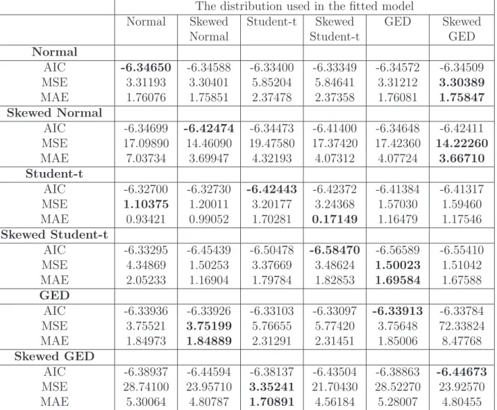
We fit each data set by the same order of the GARCH model where the data were simulated from, with six different error distributions respectively. Then compare the values of AIC given by each fitting and determine which model is the best fitted model for the underlying data set. We also evaluate the out-of-sample 1 step ahead forecasting on conditional volatility and compare the performance of each GARCH model with different error distributions measured by MSE and MAE. The results are shown in Tables 1 and 2.
From Tables 1 and 2, we can see that the true model is always the best fitted model in terms of the AIC criterion but the true model does not necessarily provide the minimum values of MSE and MAE and might not produce the best performance of forecasting volatility. For this particular sample, our simulation study shows that the statement “the best fitted model does not necessarily provide the best forecast on volatility” also holds for higher order of GARCH models.
Shamiri and Isa (2009) argue that there are several plausible models that we can select to use for our forecast and we should not be fooled into thinking that the one with the best fit is the one that will forecast the best. However, how much difference between the best forecast and the forecast given by the best fitted model? To investigate this question, for each of the six
different distribution of εt we independently simulated 100 samples from (3.3). Each sample
has size 6,536. The first 3,535 observations were considered as in-sample data and the remains were considered as out-sample data. For each set of simulated data, we fit the data by models with the six different error distributions respectively, and then calculate the value of MSE and MAE. We carry out pair t-test on the following hypothesis :
H0 : µa−µb = 0
H1 : µa−µb >0
where
µa denotes the mean of MSE (MAE) given by the best fitted model
µb denotes the mean of MSE (MAE) given by the best performance model
The reason to carry out this test is to check if the mean of MSE and MAE from the best fitted model are statistically significantly larger than the mean of MSE and MAE from the best performance model. If the null hypothesis cannot be rejected, it will mean that statistically the best performance model will not provide better volatility forecast than the best fitted model in terms of MSE(MAE) value. The P-values of the positive one tail paired t-test for 1-step and 10-step ahead forecast are shown in Table 3.
Table 1: AIC, MSE and MAE for Simulated Data from GARCH(1,3) The distribution used in the fitted model
Normal Skewed Student-t Skewed GED Skewed
Normal Student-t GED
Normal AIC -6.39728 -6.39673 -6.38562 -6.38507 -6.39678 -6.39622 MSE 33.27150 33.19940 39.41210 39.40620 32.80390 32.73420 MAE 5.76153 5.75527 6.27168 6.27122 5.72081 5.71471 Skewed Normal AIC -6.46464 -6.52380 -6.45955 -6.51125 -6.46409 -6.52332 MSE 1.69244 1.96543 2.58870 0.74882 1.69292 1.92887 MAE 1.24786 1.36565 1.56406 0.80091 1.24806 1.35239 Student-t AIC -6.35970 -6.36029 -6.47920 -6.47864 -6.46384 -6.46331 MSE 0.06376 0.07311 0.07454 4.53249 6.78319 6.73794 MAE 0.13589 0.21205 0.21138 2.11192 2.59203 2.58324 Skewed Student-t AIC -6.37249 -6.49380 -6.53352 -6.60656 -6.57894 -6.57441 MSE 0.18411 22.03428 1.32608 2.91688 0.17645 0.17655 MAE 0.28982 4.68293 1.09884 1.67549 0.28451 0.28541 GED AIC -6.38848 -6.38847 -6.37966 -6.37958 -6.38870 -6.38831 MSE 50.33190 50.40620 6.83721 47.55250 50.10220 50.18850 MAE 7.08312 7.08836 2.58594 6.88431 7.06691 7.07302 Skewed GED AIC -6.44193 -6.50376 -6.43582 -6.49304 -6.44138 -6.50432 MSE 7.06841 12.10115 7.69763 49.95989 7.13673 12.16423 MAE 2.63916 3.46648 2.75687 7.06309 2.65211 3.47556
Notes: MSE (×10−10) and MAE (×10−5) . Bold value in each row is the minimum value
Table 3 shows that all the tests are not significant. It indicates that, although based on the outcomes in Tables 1 and 2, the best fitted GARCH model does not provide the best volatility forecast. Therefore, the best fitted model is still able to make the reasonable forecast on volatility.
4
Empirical studies
Our simulation studies in previous section indicated that sometimes the best fitted model might not necessarily provide the minimum values of MSE and MAE and might not necessarily produce the best performance of forecasting volatility. However, the best fitted model is still able to provide a reasonable forecast on volatility. In this section, we want to further find out
Table 2: AIC, MSE and MAE for Simulated Data from GARCH(2,1) The distribution used in the fitted model
Normal Skewed Student-t Skewed GED Skewed
Normal Student-t GED
Normal AIC -6.34650 -6.34588 -6.33400 -6.33349 -6.34572 -6.34509 MSE 3.31193 3.30401 5.85204 5.84641 3.31212 3.30389 MAE 1.76076 1.75851 2.37478 2.37358 1.76081 1.75847 Skewed Normal AIC -6.34699 -6.42474 -6.34473 -6.41400 -6.34648 -6.42411 MSE 17.09890 14.46090 19.47580 17.37420 17.42360 14.22260 MAE 7.03734 3.69947 4.32193 4.07312 4.07724 3.66710 Student-t AIC -6.32700 -6.32730 -6.42443 -6.42372 -6.41384 -6.41317 MSE 1.10375 1.20011 3.20177 3.24368 1.57030 1.59460 MAE 0.93421 0.99052 1.70281 0.17149 1.16479 1.17546 Skewed Student-t AIC -6.33295 -6.45439 -6.50478 -6.58470 -6.56589 -6.55410 MSE 4.34869 1.50253 3.37669 3.48624 1.50023 1.51042 MAE 2.05233 1.16904 1.79784 1.82853 1.69584 1.67588 GED AIC -6.33936 -6.33926 -6.33103 -6.33097 -6.33913 -6.33784 MSE 3.75521 3.75199 5.76655 5.77420 3.75648 72.33824 MAE 1.84973 1.84889 2.31291 2.31451 1.85006 8.47768 Skewed GED AIC -6.38937 -6.44594 -6.38137 -6.43504 -6.38863 -6.44673 MSE 28.74100 23.95710 3.35241 21.70430 28.52270 23.92570 MAE 5.30064 4.80787 1.70891 4.56184 5.28007 4.80455 Notes: MSE (×10−10) and MAE (×10−5), Bold value in each row is the minimum value
Table 3: The P-values of Paired Test result between the best fitted model and the best perfor-mance model given by samples from GARCH(1,3)
1-step 10-step The best fitted MSE MAE MSE MAE
model N 0.3254 0.2517 0.3452 0.3543 SN 0.5871 0.9945 0.9845 0.9541 STD 0.8124 0.2641 0.9802 0.9678 SSTD 0.1934 0.3454 0.3546 0.2276 GED 0.0842 0.1104 0.1489 0.2978 SGED 0.3891 0.4512 0.3845 0.3312
whether the best fitted is appropriate to be used for forecast on volatility based on the real data.
4.1
Descriptive statistics
The summary statistics of return seriesrt for SET, KLCI and STI are presented in Table 4.
It shows that the mean of the returns for SET is slightly larger than the means of the returns for KLCI and STI markets. Both of the return series for SET and KLCI display negative skewness while the STI shows the positive skewness. All return series are leptokurtic and normality test for all return series are firmly rejected by the Jarque-Bera statistics. All return series have non-normal distributions.
Table 4: Summary Statistics for returns
Sample Mean (×10−3) Standard Deviation Skewness Excess Kurtosis Jarque-Bera
SET 6,536 0.289 0.01562 -0.06808 7.9577 17220∗∗∗
KLCI 3,880 -0.030 0.01554 -0.43354 40.7329 267574∗∗∗
STI 5,407 -0.200 0.01331 0.11628 8.3077 15526∗∗∗
SET daily return
SET 0 1000 3000 5000 −0.15 −0.10 −0.05 0.00 0.05 0.10
KLCI daily return
KLCI 0 1000 2000 3000 4000 −0.2 −0.1 0.0 0.1 0.2
STI daily return
STI 0 1000 3000 5000 −0.10 −0.05 0.00 0.05 0.10
Figure 1: The daily return of SET, KLCI and STI
Figure 1 shows the time series plots of the daily returns for SET, KLCI and STI respec-tively. Volatility clustering phenomenon are clearly observed from the plots. It indicates that GARCH models may be appropriate models for explaining these data.
4.2
In-sample parameter estimation and model diagnostics
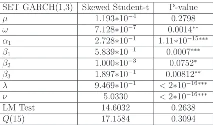
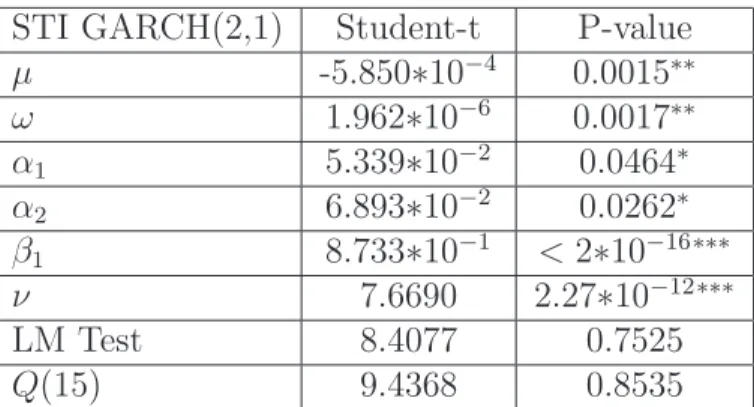
R package “Garch” is used to find the best fitted GARCH model among the models with different error distributions for in sample data and the estimation of parameters in the model. According to the results of sensitivity analysis, we found that changing error distributions does not change the order of the best fitted GARCH model (the reports are missing from this paper). Therefore, to save time in analysis processes, the orders of the best fitted model with different error distributions are chosen as the best fitted model with normal distribution. It was found that GARCH (1,3), GARCH(1,1) and GARCH(2,1) are appropriate for SET, KLCI and STI respectively. Then we apply GARCH(1,3), GARCH(1,1) and GARCH(2,1) to SET, KLCI and STI respectively, by assigning the six different distributions to the error in the models. The AIC values given by different models with different error distributions are reported in Table 5. Based on AIC criterion, GARCH(1,3) with error distribution SSTD is the best fitted GARCH model for SET, GARCH(1,1) with GED for KLCI and GARCH(2,1) with STD for STI.
Table 5: The AIC values given by models with different error distributions
AIC Normal Skewd normal Student-t Skewed Student-t GED Skewed GED SET -6.4703 -6.4749 -6.5421 -6.5432 -6.5376 -6.5409 KLCI -6.9142 -6.9137 -6.9583 -6.9575 -6.9608 -6.9596 STI -6.0739 -6.0735 -6.1104 -6.1100 -6.1061 -6.1058
Tables 6-8 show the estimates of parameters in each of the best fitted GARCH models, as well as the test statistics given by Lagrange Multiplier Test (LM test) and Ljung-Box Q
statistic.
Table 6: Estimated parameters and diagnostic of GARCH(1,3)-SSTD model for SET SET GARCH(1,3) Skewed Student-t P-value
µ 1.193∗10−4 0.2798 ω 7.128∗10−7 0.0014∗∗ α1 2.728∗10−1 1.11∗10−15∗∗∗ β1 5.839∗10−1 0.0007∗∗∗ β2 1.000∗10−3 0.0752∗ β3 1.897∗10−1 0.00812∗∗ λ 9.469∗10−1 <2∗10−16∗∗∗ ν 5.0330 <2∗10−16∗∗∗ LM Test 14.6032 0.2638 Q(15) 17.1584 0.3094
Table 7: Estimated parameters and diagnostic of GARCH(1,1)-GED model for KLCI KLCI GARCH(1,1) GED P-value
µ -5.005∗10−4 0.0004∗∗∗ ω 8.607∗10−7 0.0259∗ α1 1.136∗10−1 1.11∗10−7∗∗∗ β1 8.809∗10−1 <2∗10−16∗∗∗ ν 1.3110 <2∗10−16∗∗∗ LM Test 15.2401 0.2286 Q(15) 15.3440 0.4269
Table 8: Estimated parameters and diagnostic of GARCH(2,1)-STD model for STI STI GARCH(2,1) Student-t P-value
µ -5.850∗10−4 0.0015∗∗ ω 1.962∗10−6 0.0017∗∗ α1 5.339∗10−2 0.0464∗ α2 6.893∗10−2 0.0262∗ β1 8.733∗10−1 <2∗10−16∗∗∗ ν 7.6690 2.27∗10−12∗∗∗ LM Test 8.4077 0.7525 Q(15) 9.4368 0.8535
All parameters in GARCH(1,3), GARCH(1,1) and GARCH (2,1) for SET, KLCI and STI respectively are significant at 5% level. For each index data set, LM test supports the absence of ARCH effect in the residuals and the value of Q statistic is not significant. It shows that all the best fitted GARCH models are sufficient to correct the serial correlation of the returns series in the conditional variance equation (Liu and Hung 2010).
4.3
The performance of volatility forecasting
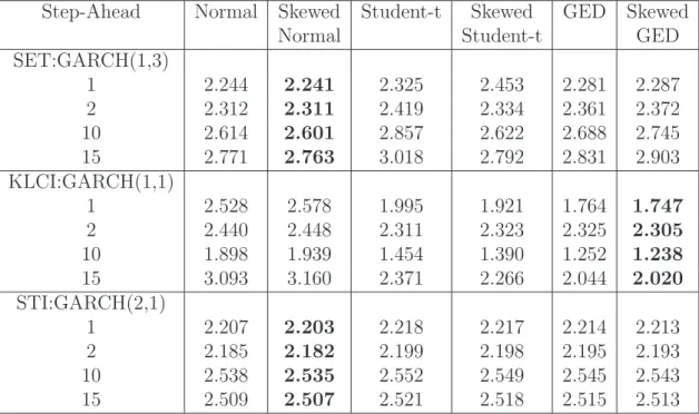
In this section, we adopt the best fitted models for SET, KLCI and STI in Section 4.2. By taking the same order of model and replacing the error distribution by other distributions mentioned in Section 2.2, we obtain six different fitted models for each index. Then we use each of these models to make out-sample forecasts. The performances of 1,2,10 and 15 steps ahead forecasts are evaluated and reported in Tables 9 and 10.
Table 9: Out-of-sample volatility forecasting evaluated by MSE
Step-Ahead Normal Skewed Student-t Skewed GED Skewed
Normal Student-t GED
SET:GARCH(1,3) 1 2.561 2.551 2.560 2.553 2.557 2.543 2 2.534 2.524 2.546 2.539 2.539 2.525 10 2.995 2.992 3.139 3.011 3.033 3.058 15 2.985 2.982 3.207 3.004 3.028 3.084 KLCI:GARCH(1,1) 1 6.847 7.105 4.390 4.096 3.471 3.468 2 1.050 1.051 1.032 1.032 1.035 1.027 10 3.614 3.771 2.126 1.942 1.561 1.544 15 9.586 5.001 5.639 5.153 4.122 4.096 STI:GARCH(2,1) 1 1.929 1.922 1.926 1.934 1.933 1.929 2 1.927 1.918 1.933 1.929 1.928 1.924 10 2.694 2.688 2.710 2.708 2.703 2.701 15 2.629 2.624 2.644 2.643 2.637 2.636
Notes: The reported value is multiplied by (×10−7). The minimum value of MSE in the same raw is in bold.
Table 10: Out-of-sample volatility forecasting evaluated by MAE
Step-Ahead Normal Skewed Student-t Skewed GED Skewed
Normal Student-t GED
SET:GARCH(1,3) 1 2.244 2.241 2.325 2.453 2.281 2.287 2 2.312 2.311 2.419 2.334 2.361 2.372 10 2.614 2.601 2.857 2.622 2.688 2.745 15 2.771 2.763 3.018 2.792 2.831 2.903 KLCI:GARCH(1,1) 1 2.528 2.578 1.995 1.921 1.764 1.747 2 2.440 2.448 2.311 2.323 2.325 2.305 10 1.898 1.939 1.454 1.390 1.252 1.238 15 3.093 3.160 2.371 2.266 2.044 2.020 STI:GARCH(2,1) 1 2.207 2.203 2.218 2.217 2.214 2.213 2 2.185 2.182 2.199 2.198 2.195 2.193 10 2.538 2.535 2.552 2.549 2.545 2.543 15 2.509 2.507 2.521 2.518 2.515 2.513
Notes: The reported value is multiplied by (×10−7). The minimum value of MAE in the same raw is in bold.
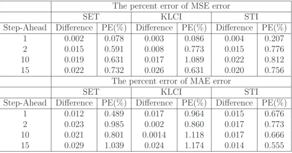
Table 11: The percent error of MSE and MAE given by the best fitted model and the best performance model
The percent error of MSE error
SET KLCI STI
Step-Ahead Difference PE(%) Difference PE(%) Difference PE(%)
1 0.002 0.078 0.003 0.086 0.004 0.207
2 0.015 0.591 0.008 0.773 0.015 0.776
10 0.019 0.631 0.017 1.089 0.022 0.812
15 0.022 0.732 0.026 0.631 0.020 0.756
The percent error of MAE error
SET KLCI STI
Step-Ahead Difference PE(%) Difference PE(%) Difference PE(%)
1 0.012 0.489 0.017 0.964 0.015 0.676
2 0.023 0.985 0.002 0.860 0.017 0.773
10 0.021 0.801 0.0014 1.118 0.017 0.666
15 0.029 1.039 0.024 1.174 0.014 0.555
provide the best volatility forecasts in terms of the values of MSE and MAE. To investigate the different of the values of MSE(MAE) given by the best fitted model and the best performance model, we evaluate the Percent Error (PE) of MSE(MAE) for each underlying cases where PE is defined as follows :
P E = A−B
A ×100% ,
where
A denotes MSE (MAE) given by the best fitted model
B denotes MSE (MAE) given by best performance model
The PE values are reported in Table 11. It shows that the majority of PE values are small and less than 1.2%. It indicates that MSE(MAE) given by the best fitted model is not statistically different from that given by the best performance model. In practical situations, we still can use the best fitted model for volatility forecasting.
5
Conclusion
This paper investigates the volatility forecasting capability of GARCH(p,q) models with six different type of error distributions and apply them to three South East Asian emerging stock
markets. Our results show that a GARCH(p,q) model with non-normal error distributions tends to provide better out-of-sample forecast performance than a GARCH(p,q) model with normal error distribution.
Simulation and empirical studies show that MSE(MAE) given by the best fitted model is insignificantly different from that given by the best forecast performance model. Since it is not practicable to identify the best performance model in practice, this study clearly demonstrates that it is reliable to use the best fitted model for volatility forecasting.
References
[1] Awartani, B.M.A. and V. Corradi. (2005). Predicting the volatility of the S&P-500 stock index via GARCH models: the role of asymmetries.International Journal of Forecasting,
21, 167-183.
[2] Bali, T.G. (2007). Modeling the dynamics of interest rate volatility with skewed fat-tailed distribution.Annals of Operations Research, 151, 151-178.
[3] Bollerslev, T. (1986). Generalized autoregressive conditional heteroskedasticity. Journal of Econometrics, 31, 307-321.
[4] Chuang, Y., J.R. Lu and P.H. Lee (2007). Forecasting volatility in the financial markets: a comparison of alternative distributional assumptions.Applied Financial Economics, 17, 1051-1060.
[5] Cont, R. (2001). Empirical properties of asset returns: stylized facts and statistical issues.
Quantitative Finance, 1, 223-236.
[6] Curto, J.D. and J.C. Pinto (2009). Modeling stock markets’volatility using GARCH mod-els with Normal,Student’s t and stable Paretian distributions. Staistical Papers,50, 311-321.
[7] Engle, R.F.(1982). Autoregressive conditional heteroskedasticity with estimates of the variance of U.K. Inflation. Econometrica, 50 ,987-1007.
[8] Glosten, L.R., R. Jagannathan and D.E. Runkle. (1993). On the relation between ex-pected value and the volatility of the normal excess return on stocks.Journal of Finance,
48, 1779-1801.
[9] Gokcan, S. (2000). Forecasting volatility of emerging stock market: linear versus non-linear GARCH models. Journal of Forecasting, 19 , 499-504.
[10] Hansen, B.E. (1994). Autoregressive conditional density estimation. International Eco-nomic Review, 35, 730-750.
[11] Komain, J. (2007). Behavior of stock market index in the stock exchange of Thailand.
[12] Lee, Y.H. and T.Y. Pai. (2010). REIT volatility prediction for skew-GED distribution of the GARCH model.Expert Systems with Applications, 37, 4737-4741.
[13] Liu, H.C. and J.C. Hung. (2010). Forecasting S&P-100 stock index volatility: The role of volatility asymmetry and distributional assumption in GARCH models. Expert Systems with Applications, 37, 4928-4934.
[14] Liu, H.C., Y.H. Lee and M.C. Lee. (2009). Forecasting China stock markets volatility via GARCH models under skewed-GED distribution.Journal of Money, Investment and Banking, 7, 5-15.
[15] Sentana, E. (1995). Quadratic ARCH models.Review of Economic Studeis, 62, 639-661.
[16] Shamiri, A. and Z. Isa (2009). Modeling and forecasting volatility of Malaysian stock markets. Journal of Mathematics and Statistics, 3, 234-240.
[17] Zakoian, J.M. (1994). Threshold Heteroskedastic Models.Journal of Economic Dynamics and Control, 18, 931-955.