Some Practical Issues Related to the Integration of Data from Sample Surveys

Some Practical Issues Related

to the Integration of Data

from Sample Surveys

1

Poznań University of Economics, al. Niepodległości 10, Poznań, Poland. E-mail: [email protected].

2

I.e. demographic cross sections within a small geographical area (i.e. NUTS 4).

Abstract

Th e users of offi cial statistics data expect multivariate estimates at a low level of aggregation. However, due to fi nancial restrictions it is impossible to carry out studies on a sample large enough to meet the demand for low-level aggregation of results. At the same time, respondents’ burden prevents creation of long question-naires covering many aspects of socio-economic life.

Statistical methods for data integration seem to provide a solution to such problems. Th ese methods involve fusion of distinct data sources to be available in one set, which enables joint observation of variables from both fi les and estimations based on the sample size being the sum of sizes of integrated sources.

Keywords

Data fusion, data integration, multiple imputation, quality assessment, statistical matching, sample survey

JEL code

C02, C18, C31, C63, C83

INTRODUCTION

Offi cial statistics institutions conduct many sample surveys in order to respond to the demand for in-formation reported by a number of diff erent public and private institutions. Th e substantive content of the surveys derives not only from the needs of the recipients, but also from international commit-ments enabling comparative analysis of diff erent socio-economic phenomena in the European Union. At the same time due to the very high costs a sample size in the studies does not allow for generalization of the results in the detailed cross-sections, while the respondent burden which results in refusals and missing data enforces design of relatively short questionnaires. Hence, a statistical inference for small domains2 is impossible (due to large sampling error) and none of the studies cover all the aspects of the socio-economic phenomena. For these reasons the current process of modernization of the statistical infrastructure includes increasing the effi ciency of reporting systems through the integration of statisti-cal information from available data sources (Leulescu, Agafi tei, 2013).

Statistical data integration methods can provide a response to the problems of disjoint observation of variables in the sample surveys, and also allow for the estimation of better quality for small domains. For several years they are considered the subject of public statistics, and Eurostat in particular. Th e projects

like CENEX-ISAD (CENEX 2006) or Data Integration (ESSnet on Data Integration 2011) improved and disseminated the methodology of the statistical data integration.

Statistical matching (data fusion) is a methodological approach that provides a joint observation of variables not jointly observed in two (or more) datasets. Potential benefi ts of this approach lies in the possibility of increasing the analytical capacity of existing data sources without increasing the cost of research and the burden on respondents.

Th e scope of this paper is to identify some practical issues related to the integration of data from sam-ple surveys with statistical matching method like in Raessler (2002) and D’Orazio et al. (2006). In fi rst section the statistical matching framework will be described with particular emphasis on combining the microdata sets. Th e next section will deal with the methodology of merging two sample survey data fi les with some practical remarks. Especially approaches to harmonizing and concatenation of datasets will be shown as well as methods of the missing data imputation. In the third section integration of data from two sample surveys – Household Budget Survey (HBS) and European Union Statistics on Income and Living Conditions (EU-SILC) – will be presented with particular emphasis on the quality and effi -ciency of the algorithms used. At the end the general conclusions will be presented.

1 STATISTICAL MATCHING OVERVIEW

Statistical matching is a group of statistical methods for the integration of two (or more) data sources (usually originating from sample surveys) referring to the same target population. Th e aim of the inte-gration is the joint observation of variables not jointly observed in any of the sources and the possibility to make inference on their joint distribution.

1.1 Matching scheme

In each of the input datasets (labeled A and B) a vector of variables of the same (or similar) defi nitions and categories is available. Th ese are so called common variables (labeled as x). Dataset A contains also a vector of variables which is observed only in this dataset (labeled y) and, analogically, dataset B contains also a vector of variables which is observed only in this dataset (labeled z). Variables y and z are called distinct (or target) variables. Since the probability of selection the same unit to two (or more) samples simultaneously is close to zero, it is assumed that the input datasets are disjoint.

(x,y,z) are random variables with the density function f(x,y,z). It is assumed that x=(X1 ,…, XP)', y=(Y1 ,…,YQ ), z=(Z1 , …, ZR) are random variables vectors of a size P, Q and R respectively. It is also as-sumed that A and B are two independent samples consisting of nA and nB independently drawn units (Di Zio, 2007).

Vector (xaA , yaA ) = (xaA 1 ,... , x aA P ; yaA ,..., yaA Q), a =1,…,na, consists of the observed values of variables for units in dataset A. Analogically, vector (xbB , zbB ) = (xbB 1,... , x bB P ; zbB ,..., ybB R), where b=1,…,nb, consists of the ob-served values of variables for units in dataset B (see Scheme 1).

Both A and B datasets should contain information about the same target population. Hence, the type of statistical/observation unit should also be the same (i.e. person, household etc.). Th e reference pe-riods also ought to be similar. Should any of mentioned conditions failed, harmonization needs to be performed. If it is impossible to harmonize datasets (diff erent populations, inconsistent unit types etc.), integration is impossible to conduct.

Th e statistical matching algorithm is initialized with the choice of target variables. Th ese are variables selected from vector of distinct variables y (and z) which are going to be merged with data in set B (A). Th e dataset to which, in particular integration step, variables are being matched is called recipient, while the dataset which variables are being matched from is called donor. Th e choice of the target variables is usually dictated by the information needs, and depending on the nature of the variables used, set of rules and methods of integration is used.

In the next step a vector of common variables x is identifi ed. From that vector, according to particu-lar target variables, a set of matching variables is being chosen xM x. Usually variables that explain

the most of the variance of the target variable are being chosen. Th e relationship between common and target variables is usually not one-dimensional. Hence, the matching variables are usually being chosen using multidimensional methods like stepwise regression, cluster analysis or classifi cation and regres-sion trees (CART).

1.2 Conditional Independence Assumption

Since variables y and z are not jointly observed in any sources, in the estimation of the relationship between these characteristics it is usually assumed that y and z are conditionally independent given x (Raessler, 2004, D’Orazio et al., 2006, Moriarity, 2009). It is called conditional independence assumption

(CIA) and under CIA the density function of (x, y, z) has the following property:

, (1) where f(Y | X) is a conditional density function of y given x, f Z | X is a conditional density function of z given

x, and fX is a marginal density of x. When the assumption of conditional independence is true,

informa-tion about marginal distribuinforma-tion of x and about relainforma-tionships between x and y as well as x and z is suf-fi cient to estimate (1). Th at information can be derived from A and B datasets.

It is worth underlining that the veracity of the CIA cannot be tested using information from AB

solely. False assumption may lead to biased estimates. In order to obtain a point density estimate f(x,y,z) it is necessary to refer to external sources of information. Singh et al. (1993) determined two types of such sources:

– third database C in which (x, y, z) or (y, z) are jointly observed, – reliable values of unknown relations between (y, z|x) or (y, z). Scheme 1 Initial data in statistical matching

Dataset A ǥ … ǥ ǥ ǥ ǥ ǥ ǥ ǥ ǥ ǥ ǥ ǥ ǥ ǥ ǥ ǥ ǥ ǥ ǥ … … Dataset B ǥ ǥ ǥ ǥ ǥ ǥ ǥ ǥ _{ǥ ǥ} ǥ ǥ ǥ ǥ ǥ ǥ ǥ ǥ Source: Di Zio (2007) ǡǡൌ ȁȁ ȁȁ , ׊ אǡאǡא

In practice, many problems with the dataset C may occur. It may be inconsistent with A and B in terms of population, defi nitions or reference period. Conducting a new study in order to obtain joint observa-tion of (x, y, z) or (y, z) raises problems of economical (cost and time to carry out research) and statisti-cal (new dataset can be characterized by missing data and random and/or non-random errors) nature.

When additional data sources are unavailable, uncertainty analysis is being performed (D’Orazio et al. 2006) which is a kind of interval estimation for unknown characteristics, such as correlation matrix of (y,z). Th e narrower the estimated intervals are, the better quality of the integrated data sets charac-teristics are. Th e product of application of statistical matching methods using interval estimation are, for microdata sets, family of synthetic datasets created by using a variety of reliable parameters used in the integration model.3

In conclusion, data fusion can be performed using (i) conditional independence assumption, (ii) aux-iliary (additional) data sources, (iii) uncertainty analysis.

In the works, among others, of Kadane (1978), Paas (1986) and Singh et al. (1993) it is showed that the integration with the conditional independence assumption usually leads to estimates of suffi cient quality. Th e conditional independence assumption is most commonly used because of the ease of appli-cation and, as practice shows, a good quality of integration.

2 MATCHING ALGORITHM 2.1 Datasets harmonization

Harmonization is laborious but a necessary initial step in the integration. It allows, among others, com-parison of distributions of variables from various sources and subsequent evaluation of the results of the integration. According to van der Laan (2000) 8 steps of harmonization can be distinguished (see also Scanu, 2008):

1. units defi nition harmonization; 2. reference periods harmonization; 3. population completeness analysis; 4. variables harmonization;

5. variables categories harmonization; 6. measurement error correction; 7. handling missing data; 8. creation of derivative variables.

Without loss of generality, the above mentioned steps can be grouped into 2 categories: (i) compat-ibility of the population and units (1–3), (ii) harmonization of variables (4–8).

Th e integration of the two data sources is justifi ed when: (i) reference periods of the surveys are con-sistent, (ii) populations in the surveys are the same or diff erent but overlapping.

In the case of non-consistent reference periods, they should be corrected (i.e. by performing demo-graphic projections).

If the populations are diff erent but overlapping, in the integrated datasets (labeled as A i B) subsets

A1 and B1 must be extracted, in such a way that they contain a common part of the population. It has to be verifi ed whether the obtained subsamples are representative for the surveyed population (Scanu, 2008). If the verifi cation is successful, subsets A1 and B1 can be integrated.

When the two datasets refer to two diff erent (disjoint) populations, none of the methods will be proper.

3

Another approach is solely an estimate of specifi c relations (e.g. correlation, regression coeffi cients, contingency table) between vectors of variables Y and Z, without creating a synthetic microdata set – the so-called macro approach (D’Orazio et al., 2006).

Common variables should be fully consistent. It means that both defi nitions and distributions ought to be at least very similar. In the datasets from diff erent sources meeting both of these conditions in full may be diffi cult. Th e most common problems which can be encountered here are the following:

– diff erent defi nitions of variables and occurrence of diff erent categories, – missing data,

– distribution of the same variables among populations.

In the case of non-consistent defi nitions and/or categories of common variables, there are three types of variables:

1. Th e variables for which there is no possibility for harmonization

Such variables should not be regarded as ‘common’ and therefore they should not be considered as matching variables at all. Th is situation happens quite oft en, especially when the datasets come from diff erent institutions.

2. Th e variables that can be harmonized by modifi cation of their categories

Qualitative characteristics oft en contain many variants. Th eir harmonization is usually done by aggrega-tion in such a way that derivative variants are created. Th ese are consistent in both datasets (i.e. education ‘primary’ and ‘no education’ can be aggregated to ‘primary or no education’). Aggregation of categories can lead to loss of information, though.

3. Th e derivative variables

In the absence of appropriate common variables or their insuffi cient number, new variables can be cre-ated by transforming other available variables. If the derived variables meet certain criteria (qualitative and defi nitional), they can be used as matching variables.

Th e common variables should also show appropriate quality. It means, among others, that they shouldn’t contain missing data. Unit non-response results in the removal of the unit from the dataset. In the case of item non-response, two ways can be distinguished: (i) using variables without missing data only, (ii) impute missing data.

Th e third issue concerns the compatibility of distributions of variables. Th is is due to the assumption that input datasets refer to the same population. In situations where the distributions of the common variables are very diff erent, it might be suspected that populations are non-consistent. More frequent situation is that the diff erences in the distributions of common variables arise from the variation of the sample.

Diff erences in the distributions can be examined by commonly used statistical tests (i.e. chi-squared test for goodness of fi t, Kolmogorov–Smirnov test, etc.). However, for large samples formal statistical tests tend to reject the hypothesis of equality of distributions or fraction even at very small diff erences. Also, most of the ‘classical’ statistical tests were constructed for a simple randomized sampling scheme, while the input datasets oft en come from studies of complex sampling scheme.

Scanu (2008) suggested so called ‘empirical approach’. Its essence is to compare the distributions of appropriate variables using visual methods and the use of some simple measures:

– for continuous variables – comparison of histograms;

– for qualitative variables – comparing fraction diff erences of the particular categories: – for ‘big’ fractions – diff erences lower than 5% are acceptable,

– for ‘small’ fractions – diff erences lower than 2% are acceptable; – for both scale and qualitative variables – total variation distance:

, (2) where wA,i and wB,i are i-th (i=1,…, k) relative frequencies of a particular variable in the integrated data-sets. In practice, it is accepted that distributions are "acceptably" compatible when Δ ≤ 6%;

– for scale variables it is possible to compare estimates of population parameters, . 2.2 Matching methods

Taxonomy of integration methods is described in detail in D’Orazio et al. (2006). For the purpose of integration of microdata sets, three frameworks are distinguished: (1) parametric, (2) non-parametric, (3) mixed. In the parametric framework, generally two techniques are used: (1) regression imputation, (2) stochastic regression.

Th e regression imputation in statistical matching is a fairly simple approach. Two models Y(X) and

Z(X) are being estimated. Th en predicted values are being imputed to B and A respectively. Th is process consists of three steps:

1. Predicted values resulting from a model:

, (3) are imputed to A.

2. Predicted values resulting from a model:

. (4) are imputed to B.

3. Datasets A and B are concatenated: S = AB; nS = nA + nB.

Th e advantage of this approach is its simplicity. Th e disadvantage is the fact that it is a single imputa-tion and the predicted values lie on the regression line.

Little and Rubin (2002) suggested to use a stochastic imputation in the statistical matching. It consists on drawing residual values for regression models obtained in such a way that:

, (5) where ea~N(0, σ ̂Z |X), and

, (6) where eb~N(0, σ ̂Y |X).

Development of the stochastic imputation method is a multiple imputation, suggested by Raessler (2002) to be used in the statistical matching framework. For the purpose of the multiple imputation m models are created. Each of the models is created using the stochastic regression method. Drawing residuals re-fl ects the sample variability and allows to perform point and interval estimation for the unknown values of missing data (which is also a pro-solution for the problem of uncertainty, as described in section 1.2).

Th e imputation estimator for each of t (t=1,2,…,m) models is , where Uobs are observed values, and are imputed missing data (Raessler 2002). Th e variance of the estimator is formulated as . Th e point estimate of the multiple imputations is an arithmetic mean:

. (7)

“Between-imputation” variance is estimated by formula:

(8) ̂ሺሻൌ"#൅$%, ൌ ͳǡʹǡ ǥ ǡ i.e. , , #ሺሻൌ"#൅$% , ൌ ͳǡʹǡ ǥ ǡ ̃ሺሻൌ̂ሺሻ൅(ൌ"#൅$% ൌ_# ∑ሺ./ െ./!"ሻ ./ሺሻ_{ൌ./ሺ0 ǡ0} ሺሻሻ 0ሺሻሻ 123 ./ ൌ123ሺ./ሺ0 ǡ0ሺሻሻሻ ./!"ൌ∑./ ൌ_# ∑ሺ./ െ./!"ሻ

and “within-imputation” variance is estimated by:

. (9) Total variance is a sum of between- and within-variance modifi ed by m + 1, to refl ect the uncertainty about the true values of imputed missing data: m

. (10)

Interval estimates are based on t-distribution:

(11)

with degrees of freedom:

. (12) Th e main advantage of the parametric approach is the ‘economy’ of the model – a small number of predictors explains a large part of the variance of the target variables. Among the disadvantages a need of model specifi cation can be mentioned. Poorly constructed imputation model can generate results with poor quality. In addition, the imputed values are artifi cial, i.e. resulting solely from the model, not having their counterparts in reality. Th is problem is usually solved by the use of a mixed approach.

Th e non-parametric framework in data fusion is related to hot deck imputation methods (Singh et al., 1993). In practice, two groups of methods are most commonly used: (1) random imputation, (2) near-est neighbor matching.

Random imputation includes random draws of values of Z(Y) variables from dataset B(A) to A(B). To maintain maximum distribution compliance of target variables, datasets are divided into many ho-mogeneous groups, on the basis of categories of chosen common variables xG x. Random matching

proceeds within the designated groups.

Nearest neighbor method involves choosing for each record in the set A(B) most similar record of the set B(A). ‘Similarity’ is measured as the distance between the values of matching variables:

. (13)

Hot deck imputation methods are commonly used in practice. Th eir main advantage is that imputed values are ‘life’ – they are empirically observed. Also, the non-parametric methods do not need a model specifi cation and are quite simple in use. Main disadvantages is computational burden (each record in one dataset is compared to each record in the other dataset4) as well as only single values are being imputed.

Th e mixed methods combine advantages of parametric and non-parametric methods and alleviate their disadvantages. Most commonly (D’Orazio et al., 2006) mixed methods are described as a two-step algorithm:

1. multiple imputation with draws based on conditional predictive distribution;

2. empirical values with the shortest distance from the imputed values are matched: dab(z̃a , zb). Such an approach ensures that the imputed values are real as well as the multiple imputation provides possibility of uncertainty analysis. Commonly used method is predictive mean matching (Landerman et. al., 1997). 4ൌ∑ 123 ./ 5ൌ4൅$ ./!"െ-%ǡ√5൏.൏./!"൅-%ǡ√5 1ൌ ሺ,െ ͳሻሺͳ ൅ & ሺ$ሻሻ 7 ൌ!Ǥǡ!Ǥ 4

2.3 Integration of data from complex sample surveys

In sample surveys carried out by the offi cial statistics most frequently complex (multi-stage) sampling schemes are used. Rubin (1986) proposed a solution taking into account the sampling schemes of in-tegrated studies. Th e idea is to transform inclusion probabilities of particular units in such a way that integrated repository refl ects the size of the population (N).

Th e inclusion probability of each -th unit in the integrated dataset is the sum of the inclusion prob-abilities in and surveys minus the probability of selecting the units for both surveys simultaneously:

. (14) Since normally sample size is a very small percentage of the size of the entire population, and, in addi-tion, the institutions carrying out the measurement, ensuring that respondents were not overly burdened with obligations arising from the study, tend not to take into account one unit in several studies over a given period, equation (1) can be simplifi ed as:

. (15) Resulting from the sampling scheme survey weight is the inverse of inclusion probability. In an inte-grated dataset it will have the form:

. (16)

In practice, however, generally the inclusion probability is not available in the fi nal dataset, but it con-tains computed weights (e.g. calibrated due to missing data). For the synthetic data set corresponded to the size the target population, the transformation of weights by the following formula is made:

, (17) where:

– harmonized analytical weight for i-th unit in the integrated data set, – original analytical weight,

N – population size.

Before matching procedure is performed, datasets are concatenated (S = AB; nS = nA + nB) and an imputation model, which takes into account survey weights is specifi ed.

2.4 Quality assessment

Quality assessment of joint distribution of variables never jointly observed is a non-trivial task. Barr and Turner (1990) as well as Rodgers (1984) suggested relatively simple measures of quality assessment of integrated dataset S = AB – a comparison of basic statistics (mean, standard deviation etc.) in donor and integrated datasets.

Raessler (2002) proposed a more complex way of the quality evaluation, called an ‘integration valid-ity’. It consist of a verifi cation of four ‘validity levels’:

1. A reproduction of true, unknown values of Z(Y) in the recipient fi le – in result a ‘hit ratio’ coef-fi cient can be calculated. When a true value is replicated, a is noted. Th e coeffi cient is a ratio be-tween number of ‘hits’ and the number of imputed values.

2. A joint distribution preservation – a true unknown joint distribution of (x,y,z) is preserved in an integrated dataset.

3. A covariance structure c͠ov(x,y,z) = cov(x,y,z) is refl ected in the integrated dataset as well as mar-ginal distribution f̃XY = fXY and f̃XZ = fXZ are copied.

8׫ǡൌ8ǡ൅8ǡെ8תǡ 8׫ǡ؆8ǡ൅8ǡ _׫ൌ₍ ׫ǡ ′ ׫ൌ )_׫ ∑)׫) ′ ׫ )_׫

All above mentioned ‘levels’ can be evaluated only by the simulation study. Empirical evaluation, in the situation of no joint observation of target variables, is impossible.

4. Marginal distribution of Z(Y) as well as joint distribution of x and z (x and y) of the donor fi le should be similar in the integrated dataset.

In practice, most commonly used is the one suggested by German Association of Media Analysis (Raessler, 2002):

1. comparing the empirical distribution of target variables included in the integrated fi le with the one in the recipient and the donor fi les,

2. comparing the joint distribution fX,Z (fX,Y) observed in donor fi le with the joint distribution f̃X,Z

(f̃X,Y) observed in the integrated fi le.

3. EMPIRICAL STUDY

In this research the issues of empirical verifi cation of selected statistical methods for data integration, evaluation of the quality of a combination of various sources, integrated data quality assessment and compliance and accuracy of the estimation are carried out.

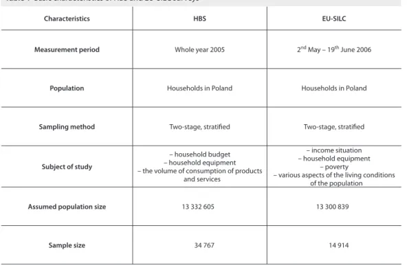
Due to the availability of data, as well as the content, the empirical study was conducted using sets of the Household Budget Survey (2005) and the European Union Statistics on Income and Living Condi-tions (2006).5

5

A dataset of 2006 was used due to the fact that the reference period of households’ income in the EU-SILC survey was set in the year preceding the survey. It was assumed that the other variables like household equipment, living conditions and socio-demographic characteristics are less volatile in time than fi nancial categories. In this way, eff orts were made to maintain compliance of common variables of EU-SILC with HBS.

Characteristics HBS EU-SILC

Measurement period Whole year 2005 2nd _{May – 19}th _{June 2006}

Population Households in Poland Households in Poland

Sampling method Two-stage, stratifi ed Two-stage, stratifi ed

Subject of study

– household budget – household equipment – the volume of consumption of products

and services

– income situation – household equipment

– poverty

– various aspects of the living conditions of the population

Assumed population size 13 332 605 13 300 839

Sample size 34 767 14 914

Table 1 Basic characteristics of HBS and EU-SILC surveys

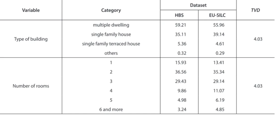
Aft er performing harmonization, the similarity of distribution of the harmonized common variables in the integrated datasets was done. For qualitative variables of total variation distance (TVD) coeffi -cient was used (see section 2.1; see Table 3). Variables with the value greater than 6% were rejected. For the quantitative variables a ratio between basic distribution parameters was calculated (see Table 4). Th e closer the value of the coeffi cient is to one, the more similar the distributions are.

For the purposes of empirical study it was decided to merge households expenditures (to EU-SILC) dataset and head of household incomes6 (to HBS fi le). Th e extension of the substantive scope of the es-timates contained among others estimation of the unknown correlation coeffi cient between household expenditure and heads of households income. Hence, the integration leads to the extension of the sub-stantive scope of the estimates. Integration includes information on households (see Table 1).

3.1 Datasets harmonization

A very important aspect is to harmonize the datasets before the integration. In both repositories variables with the same or similar defi nitions existed. Categories, however, were oft en divergent and aggregation was required to harmonize variants to the same defi nition (see Table 2). Both studies were carried out by the same institution, similar aims were guided and measurement was subject to a very similar areas of socio-economic life. It seems, therefore, that the defi nitions of their variants should be consistent not only for data integration but primarily for comparative purposes. It seems that discrepancies occurring in both studies arise from specifi c international obligations and the need for comparisons with other analogous studies carried out in other European countries.

6

As an example of a personal income of a household member which was not measured in HBS.

Table 2 Harmonization of categories of selected common variables

Variables HBS categories EU-SILC categories Harmonized categories

Type of building

1 ‘multiple dwelling’ 1 ‘detached house’ 1 ‘multiple dwelling’

2 ‘single family terraced house’ 2 ‘terraced house’ 2 ‘single-family house’

3 ‘single family detached house’ 3 ‘apartment or fl at in a building

with less than 10 dwellings’ 3 ‘single family terraced house’

4 ‘other’ 4 ‘apartment or fl at in a building

with 10 or more dwellings’ 4 ‘other’

Number of rooms

Scale variable with min=1 and

max=12 1 1

2 2

3 3

4 4

5 5

6 ‘6 and more’ 6 ‘6 and more’

Table 3 Distribution compliance assessment for selected qualitative common variables (in %) Variable Category Dataset TVD HBS EU-SILC Type of building multiple dwelling 59.21 55.96 4.03

single family house 35.11 39.14

single family terraced house 5.36 4.61

others 0.32 0.29 Number of rooms 1 15.93 13.41 4.03 2 36.56 35.34 3 29.43 29.14 4 9.86 11.07 5 4.98 6.19 6 and more 3.24 4.85

Source: Own study

Variable Statistics

Dataset _{Ratio of sample} parameters HBS EU-SILC Disposable income Mean 2 155.7 2 286.3 0.943 Variance 3 451 099.9 3 266 838.2 1.056 Standard deviation 1 857.7 1 807.4 1.028

Equivalised disposable income

Mean 1 222.8 1 288.6 0.949

Variance 991 775.5 828 935.2 1.196

Standard deviation 995.9 910.5 1.094

Table 4 Distribution compliance assessment for selected quantitative common variables

Source: Own study

3.2 Choice of matching variables

Among the common variables, for each of the target variables as the dependent variable, selection of variables was performed using the CART method. Following variables were chosen:

– for variable household expenditures: if the household has a private bathroom, if the household has a fl ushable toilet, if the household has a car, number of rooms, type of building, equivalised dis-posable income, disdis-posable income, household size;

– for variable income of head of household: if the household has a fl ushable toilet, if the household has a washing machine, if the household has a car, if the household has a TV, number of rooms, type of building, legal title to occupied apartment, equivalised disposable income, disposable income, household size.

3.3 Integration results

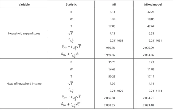
One hundred imputations were performed based on a linear regression models. Residuals were drawn us-ing Markov Chain Monte Carlo method (MCMC) (IBM SPSS Missus-ing Values 20 2011). Rubin’s approach was used to harmonize analytical weights. Both multiple imputation (MI) and mixed approach were used.

For the selected methods of integration consistent results were achieved (see Table 5 and Table 6). Designated confi dence intervals had a low spread. Additionally, through the use of interval estimation

it was possible to estimate the uncertainty of the true unknown values in the integrated dataset (assess-ment veracity of the CIA in terms of the integrated sets was impossible).

Table 5 Assessment of estimators of the arithmetic mean of variables in an integrated data set

Variable Statistic MI Mixed model

Household expenditures B 8.14 32.25 W 8.80 10.06 T 17.03 42.64 4.13 6.53 2.2414093 2.2414031 1 950.86 2 005.29 1 969.36 2 034.56

Head of household income

B 35.20 5.23 W 14.68 11.88 T 50.23 17.17 7.09 4.14 2.2414029 2.2414114 2 006.58 2 004.91 2 038.35 2 023.48 √ െǡ√ ൅ǡ√ _ǡ √ െ_ǡ √ ൅ǡ√ _ǡ

Source: Own study

Table 6 Assessment of estimators of the correlation coeffi cient of not jointly observed variables in an integrated dataset

Variable Statistic MI Mixed model

Correlation coeffi cient

ሺ ሺሻ_ሻ B 0.00006 0.00013 W 2E–15 2E–15 T 0.00006 0.00013 0.01 0.01 2.2760035 2.2760035 0.5611 0.5534 0.5849 0.5884 √ െǡ√ ൅ǡ√ _ǡ

Note: – ztransformed ρ estimate: has a normal distribution with the constant variance . The confi

dence intervals are given for ̑ρ (marked grey).

ሺ ሺሻ_{ሻ ൌ}

ೊೋሺ೟ሻ

ೊೋሺ೟ሻ

;

Source: Own study

Also, a joint observation of variables not jointly observed in any of the input databases was achieved (see Figure 1).

Figure 1 Diagram of correlation between variables not jointly observed in input sets 30 000 25 000 20 000 15 000 10 000 5 000 0 -5 000

Head of the household inc

ome

0 5 000 10 000 15 000 20 000 25 000 30 000

Total expenditure of household Note: For a convenience of illustration range of variables in the graph was reduced.

Source: Own study

Variable Region (NUTS1) HBS EU-SILC integrated x̅ S ( x̅) CV x̅ S ( x̅) CV x̅ S (x ̅) CV Household _expenditur es central 1 916 16.40 0.86 2 130 29.48 1.38 2 024 14.95 0.74 0.088 south 2 008 16.44 0.82 2 072 27.59 1.33 2 040 14.45 0.71 0.121 east 1 970 19.27 0.98 2 040 29.12 1.43 2 005 16.19 0.81 0.160 north-west 1 973 18.20 0.92 2 147 37.72 1.76 2 061 18.11 0.88 0.005 south-west 2 138 27.10 1.27 2 121 44.00 2.07 2 130 23.27 1.09 0.141 north 2 058 21.28 1.03 1 994 27.64 1.39 2 026 16.51 0.82 0.224 Head of household inc ome central 1 831 18.40 1.00 2 270 34.05 1.50 2 052 17.16 0.84 0.168 south 2 005 21.04 1.05 2 097 42.49 2.03 2 051 20.63 1.01 0.041 east 1 928 18.61 0.97 2 017 26.84 1.33 1 972 15.27 0.77 0.198 north-west 2 000 20.86 1.04 2 092 38.55 1.84 2 046 19.31 0.94 0.095 south-west 2 111 34.24 1.62 2 134 37.40 1.75 2 122 24.96 1.18 0.275 north 2 108 25.16 1.19 1 990 30.51 1.53 2 049 18.99 0.93 0.223 1 – ࢏࢔࢚ ࢋ࢓࢖

Note: Note: grey – estimates based on the imputed values, the gain measure is defi ned as: or . _{ͳ െ}೔೙೟̅ ಹಳೄ̅ ͳ െ

೔೙೟̅

ಶೆషೄ಺ಽ಴̅ Source: Own study

Table 7 Estimation of average values of matched variables [in PLN] by region with an assessment of the precision of estimate

Joint observation of variables not jointly observed was not the only gain achieved through data fusion. Th anks to the dataset concatenation approach the integrated dataset contained 49681 units (the sum of sample sizes of input datasets, see Table 1). Enlarged sample size allows to reduce the sampling error (see Table 7). Th at can be a contribution to the use of statistical data integration methods in small area estimation.

3.4 Quality assessment

Th e quality of integration was performed using German Association of Media Analysis approach (see section 2.4). Th e empirical distributions were compared by analysis of characteristics of distribution of integrated variables.

Table 8 Comparison of marginal distributions of appending variables in input and integrated datasets Variable Dataset

MI Mixed

Mean Median Std. Dev. Skewness Mean Median Std. Dev. Skewness

HH expenditures HBS 1 954.20 1 602.67 1 507.15 5.22 1 954.20 1 602.67 1 507.15 5.22 EU-SILC (imp.) 1 966.02 1 697.63 1 282.89 10.33 2 085.71 1 825.76 1 162.18 2.45 Integrated 1 960.11 1 653.46 1 399.59 7.23 2 019.92 1 720.77 1 347.46 4.4 Head of HH income HBS (imp.) 1 979.49 1 644.79 1 755.34 3.03 1 962.96 1 558.36 1 553.94 4.55 EU-SILC 2 065.48 1 566.00 1 773.33 3.13 2 065.48 1 566.00 1 773.33 3.13 Integrated 2 022.46 1 613.19 1 764.87 3.08 2 014.19 1 560.80 1 667.98 3.74

Source: Own study

Analysis of the basic distribution characteristics shows that both methods retain the essential charac-teristics of the distribution in a good manner.7 Th e statistics in the integrated dataset are always located between the values coming from input sets (see Table 8). Also the imputed with described methods values retain similar to the empirical values. It should also be noted that the MI method returns better results when one imputes from smaller to larger dataset and mixed method seems better otherwise.

Table 9 Comparison of joint distribution (correlation coeffi cient) with selected common variables in input and integrated datasets Variable Dataset MI Mixed Disposable income Equivalent income Disposable income Equivalent income HH expenditures HBS 0.588 0.484 0.588 0.484 EU-SILC (imp.) 0.855 0.677 0.872 0.675 Integrated 0.707 0.568 0.706 0.562 Head of HH income HBS (imp.) 0.965 0.937 0.873 0.834 EU-SILC 0.887 0.854 0.887 0.854 Integrated 0.926 0.896 0.877 0.839

Source: Own study

7

Formal statistical tests, due to the large sample size, always lead to the rejection of the null hypothesis. Comparison of basic characteristics as a measure of the goodness of integration was proposed by D’Orazio et al. (2006).

Analysis of selected joint distributions with chosen common variables indicates that the most consist-ent results were obtained using the mixed method (see Table 9).

It has to be noted that imputation using mixed model from EU-SILC, which has much smaller sample size, to HBS could disrupt the continuity of the variable since one record can be used more than once. In such case the MI approach seem to be better.

CONCLUSIONS

Conducted empirical study showed that the creation of the integrated data set allows to extend the sub-stantive scope compared to the input datasets. At the same time, estimation accuracy was verifi ed based on the integrated socio-economic dataset. Th e quality of the integration as well as compliance of joint and marginal distributions of target variables was assessed in the integrated dataset.

Th e integrated data repository contains information about the joint household fi nancial characteris-tics. Among others, correlation coeffi cient between two distinct variables was possible to estimate. Such characteristics was not possible to estimate in any of the input datasets. Concatenation of the input data-sets gave the opportunity to create estimates with greater accuracy

At the same time, the results of empirical research enabled the formulation of conclusions of more general nature:

harmonization of defi nitions and categories of matching variables usually comes down to creation of derivative variables with aggregated (to ‘the lowest common denominator’) categories, which naturally reduces the amount of information coming from the variable,

– without access to additional information, it is possible to construct high-quality estimators in the integrated dataset using conditional independence assumption,

– each target variable and should be analyzed separately by, among others, selection of appropriate matching variables and integration model.

In fi nal conclusion it should be assumed that the statistical method of data integration will be in-creasingly used in statistical studies. Th is is due to two main reasons. First, rising costs of conducting surveys, increasing burden on respondents resulting to missing data, may force the entities to design studies with shorter questionnaires for their subsequent integration. Second, the increase in demand for detailed information on the low level of aggregation will enforce the fusion of information from diff erent sources to increase the eff ective sample size. Statistical data integration is an opportunity to greatly enrich the methodological workshop of statistical institution in meeting the needs of recipients of information. ACKNOWLEDGMENT

Th e author gratefully acknowledges the support of the National Research Council (NCN) through its grant DEC-2011/02/A/HS6/00183.

References

BARR, R. S., TURNER, J. S. Quality issues and evidence in statistical fi le merging [w:] Data Quality Control: Th eory and

Pragmatics. New York: Marcel Dekker, 1990.

CENEX. Description of the action2006. CENEX Statistical Methodology Area “Combination of survey and administrative data”. D’ORAZIO, M., DI ZIO, M., SCANU, M. Statistical Matching. Th eory and Practice. John Wiley & Sons Ltd., England, 2006. DI ZIO, M. What is statistical matching. Course on Methods for Integration of Surveys and Administrative Data, Budapest,

Hungary, 2007.

ESSnet on Data Integration. Report on WP1. State of the art on statistical methodologies for data integration2011. ESSnet on

Data Integration, Rome.

IBM SPSS Missing Values 20. IBM White Papers, 2011.

KADANE, J. B. Some statistical problems in merging data fi les [w:] Department of Treasury, Compendium of Tax Research. Washington, DC: US Government Printing Offi ce, 1978.

LANDERMAN, L., LAND, K., PIEPER, C. An Empirical Evaluation of the Predictive Mean Matching Method for Imputing

Missing Values. Sociological Methods Research August 1997, Vol. 26, No. 1.

LEULESCU, A., AGAFITEI, M. Statistical matching: a model based approach for data integration [online]. Eurostat Meth-odologies and Working Papers, 2013. < http://epp.eurostat.ec.europa.eu/cache/ITY_OFFPUB/KS-RA-13-020/EN/KS-RA-13-020-EN.PDF>.

LITTLE, R. J. A., RUBIN, D. B. Statistical Analysis with Missing Data. Wiley, 2002.

MORIARITY, C. Statistical Properties of Statistical Matching. Data Fusion Algorithm. Saarbrucken: VDM Verlag Dr. Mueller, 2009.

PAAS, G. Statistical match: evaluation of existing procedures and improvements by using additional information [w:]

Micro-analytic Simulation Models to Support Social and Financial Policy. Amsterdam: Elsevier Science, 1986.

RAESSLER, S. Statistical Matching. A Frequentist Th eory, Practical Applications, and Alternative Bayesian Approaches. New York, USA: Springer, 2002.

RAESSLER, S. Data fusion: identifi cation problems, validity, and multiple imputation. Austrian Journal of Statistics, 2004, 33 (1–2).

RODGERS, W. L. An evaluation of statistical matching. Journal of Business and Economic Statistics, 1984, 2.

RUBIN, D. B. Statistical matching using fi le concatenation with adjusted weights and multiple imputations. Journal of

Busi-ness and Economic Statistics, 1986, 4.

SCANU, M. Some preliminary common aspects for record linkage and matching [w:] Report of WP2. Recommendations on

the use of methodologies for the integration of surveys and administrative data. CENEX-ISAD, 2008.

SINGH, A. C., MANTEL, H., KINACK, M., ROWE, G. Statistical matching: Use of auxiliary information as an alternative

to the conditional independence assumption. Survey Methodology 19, 1993.

VAN DER LAAN, P. Integrating administrative registers and household surveys. Netherlands Offi cial Statistics, Vol. 15, Summer 2000, Special Issue: Integrating administrative registers and household surveys, Statistics Netherlands, Voorburg/Heerlen.