Modeling and simulation of nanofluid transport via elastic sheets

n a n ofl ui d t r a n s p o r t vi a e l a s ti c

s h e e t s

U d di n , MJ, S o h a il, A, B e g , OA a n d Is m a il, AIM

h t t p :// dx. d oi.o r g / 1 0 . 4 0 1 5 / S 1 0 1 6 2 3 7 2 1 8 5 0 0 3 3 3

T i t l e M o d eli n g a n d si m ul a ti o n of n a n ofl ui d t r a n s p o r t vi a el a s ti c s h e e t s

A u t h o r s U d di n , MJ, S o h ail, A, B e g , OA a n d I s m ail, AIM

Typ e Ar ticl e

U RL T hi s v e r si o n is a v ail a bl e a t :

h t t p :// u sir. s alfo r d . a c . u k /i d/ e p ri n t/ 4 6 8 8 3 /

P u b l i s h e d D a t e 2 0 1 8

U S IR is a d i gi t al c oll e c ti o n of t h e r e s e a r c h o u t p u t of t h e U n iv e r si ty of S alfo r d . W h e r e c o p y ri g h t p e r m i t s , f ull t e x t m a t e r i al h el d i n t h e r e p o si t o r y is m a d e f r e ely a v ail a bl e o nli n e a n d c a n b e r e a d , d o w nl o a d e d a n d c o pi e d fo r n o

n-c o m m e r n-ci al p r iv a t e s t u d y o r r e s e a r n-c h p u r p o s e s . Pl e a s e n-c h e n-c k t h e m a n u s n-c ri p t fo r a n y f u r t h e r c o p y ri g h t r e s t r i c ti o n s .

BIOMEDICAL ENGINEERING

Editor- in- Chief

Prof. Dr. S.V. Selishchev, National Research University of Electronic Technology, Moscow, Russia. Publisher: Springer

ISSN: 0006-3398 (print version)

ISSN: 1573-8256 (electronic version)

Journal no.

10527

Accepted: April 16th _{2018 (in press)}

MODELING AND SIMULATION OF NANOFLUID

TRANSPORT VIA BIO-ELASTIC SHEETS

M.J. Uddin a, *, A. Sohail b, O. Anwar Bég c , A.I.Md. Ismail d

a American International University–Bangladesh, Banani, Dhaka 1213, Bangladesh b Department of Mathematics, COMSATS Institute of Information Technology, Lahore, Pakistan c Fluid Mechanics and Propulsion, Aeronautical and Mechanical Engineering, Room G77, Newton Building, School of Computing, Science and Engineering (CSE), University of Salford, M54WT, UK

d School of Mathematical Sciences, Universiti Sains Malaysia, 11800 Penang, Malaysia

ABSTRACT: The field of bio-nanofluidics research has spanned over the past decade with a variety of promising applications. We investigate the ``laminar boundary layer flow’’ of a Newtonian nanofluid past a moving extendable/contractable horizontal plate with surface velocity and thermal slip effects. The passively controlled nanofluid model (PCM) is considered. Such models are physically more realistic as compared to the “actively controlled models” (ACM). Using Lie symmetry group method, the governing equations are reduced by a set of highly coupled nonlinear ODE’s with thermo-solutal coupled boundary conditions. The reduced equations are solved numerically by a generalized collocation method. The influences of the emerging parameters on the local skin friction factor and the local Nusselt number are depicted numerically. The skin friction is decreased as the thermo-phoresis and buoyancy ratio parameters are decreased. The heat transfer rates reduce with thermophoresis and buoyancy ratio parameters. Velocity slip also leads to a rise in wall temperature gradient. This study is relevant to near-wall flows in nanofluid fuel cells, nano-materials processing etc.

Keywords: Passively controlled nanofluid model, Slip flow; Lie symmetry group, Collocation method;

Boundary layer; Bio-elastic sheets.

1. INTRODUCTION

There has been immense progress in the improvement of energy-proficient heat transfer fluids

over the last two decades. In this quest, nanofluids have attracted significant attention due to

their ability to enhance thermal conductivity very substantially in many different scenarios.

Choi (1995) discussed heat transfer nanofluids with more efficient thermal conductivity results

as compared to the conventional heat transfer fluids.Nanofluids are a homogenous mixture of

base fluid and nanoparticles. On the other hand some commonly used nanoparticles are

particles of metals, nitrides and carbides etc. An inspection of the current scientific literature,

nanofluids can be used in aircraft, automobiles, fuel cells and many engineering systems. Due

to nanometer sized materials nanofluids have unique physical and chemical properties.

Nanofluids are implemented in many industries e.g. in petroleum reservoir flooding (e.g.

Suleimenov et al. (2014) who showed a reduction of surface tension on an oil boundary is

attained with nanofluids), cooling of nuclear reactors, melt-spinning and manufacture of plastic

and rubber sheets. They are further known to be employed in the extrusion of a polymer sheet

from a die and crystal growth, refrigeration (e.g. Coumaressin and Palaniradja (2014),

wherein evaporator heat transfer coefficient is shown to increase with the use of nanoparticles

e.g. copper oxide), hybrid fuel cells, sterilization of materials (e.g. silver oxide nanofluids),

enhanced cooling of metallic plates in a cooling bath, treatment of paper drying systems and in

combustion fuel technologies (e.g. Sonewane et al. (2012) who consider doping of jet fuels).

The important features of the nanofluids include higher thermal conductivity as compared to

the base fluid and stable nature of the suspension. The volume fraction of nanoparticles is

usually engineered to be 3% to 5% (Das et al. 2007), so that the nanofluid exhibits mechanical

behavior similar to the base fluid. Different models have been proposed to address the large

increase in thermal conductivity. The factors responsible for the increase in thermal

conductivity in nanofluids include (a) dispersion of nanoparticles (Buongiorno 2006) (b) the

turbulence due to the presence of nanoparticles (Pak and Cho 1988) and (c) the effect of the

rotation of the nanoparticles (Xuan and Li 2003). A comprehensive theory is required for the

estimation of the thermal conductivity of a nanofluid. Theoretical models such as (

Maxwell-Garnett 1904, Wang et al. 2003) give much lower values than those acquired at the laboratory

level. It is now established (from experiments and theoretical results) that for forced convective

nanofluid flow heat transfer characteristics enhances, whereas reverse observation is noticed

in the case of natural convection. Convective heat and mass transfer of nanofluid flow have

received attention of researchers owing to it wide range of applications such as bio-convection

available models which are easily incorporated into the framework of boundary layer flows of

nanofluids are (i) the Buongiorno (2006) model in which Brownian motion and

thermophoresis effects are included and (ii) the Tiwari and Das (2007) model which can be

utilized to study the behavior of nanofluids considering the solid volume fraction. Many

investigators deployed these two models to study various flow phenomena external to various

geometries subject to various boundary conditions. As an example, Kuznetsov and Nield

(2010) obtained similarity solution for natural convection flow of a nanofluid along a vertical

plate. Nield and Kuznetsov (2009) further studied the Cheng–Minkowycz problem of natural

convection past a vertical plate in a porous medium for nanofluids. Nield and Kuznetsov

(2011) further extended the same problem for binary nanofluids, including the effects of cross

diffusion. Very recently, Kuznetsov and Nield (2014) revised their earlier model by

incorporating a passively controlled boundary condition. Reviews have been conducted of the

latest developments in nanofluid technology and are available in the papers of Wang and

Mujumdar (2007), Das and Choi (2009), Kakac and Pramuanjaroenkij (2009), Adnan et

al. (2014), Mahdi et al. (2015), Mauro et al. (2015), Ali et al. 2015, Sheikholeslami et al.

(2015) etc. and in the monographs of Tiwari and Das (2007), Sattler (2010), Murshed et al.

(2011) and Minkowycz et al. (2012). These efforts identify, not least, numerous further

problems which require mathematical (and experimental) simulation whether in terms of

nanofluid type, geometry, boundary condition or indeed combinations of these aspects.

The vast majority of investigations have generally focused analysis on natural convective flow

of nanofluids from vertical surfaces. However, the natural convective flow of nanofluids from

a horizontal surface is also of great interest in engineering devices and processes. To achieve

more physically realistic and practically applicable results, in the present article we address the

composite effects of velocity slip, thermal slip and zero mass flux boundary conditions on the

boundary layer flow of nanofluid over an upward facing horizontal sheet (plate). In addition to

the imposition of modified slip and solutal boundary conditions, sheet stretching/shrinking is

also an important characteristic in manufacture of nanomaterials (Ferdows et al. 2014), and

indeed in compliant surfaces in next-generation “green” fuel cells (Tominaka et al. 2009). An

experimental investigation in materials extrusion carried by Vleggaar (1977) revealed that the

surrounding fluid motion can be idealized by a tangentially moving boundary with a velocity

proportional to linear/nonlinear function of the distance from the slit. Hence to improve the

accuracy of wall conditions, we have incorporated the simultaneous effects of velocity slip,

nanofluid over an upward facing nonlinearly radiating horizontal stretching sheet. Lie group

analysis is used to determine the similarity form of the governing boundary layer equations.

Key parameters which influence the heat, mass and momentum transfer processes are shown

to be buoyancy ratio parameter (which is a measure of the ratio of the buoyancy force arising

due to the density difference between the nanoparticle and the base fluid and the buoyancy

force due to the thermal expansion of the base fluid), the Brownian motion parameter (which

gives information about the energy transport by Brownian diffusion) and the thermophoretic

parameter (that gives a measure of the energy transport due to thermophoresis) and their effect

on the fluid velocity and heat transfer rate are discussed. Furthermore the effect of the Lewis

number and of course multiple slip conditions on flow characteristics is also elucidated in

detail. Verification of the present collocation numerical solutions is achieved where possible

with earlier published results.

2. METHODOLOGY

2.1 Materials

A moving horizontal stretching/shrinking sheet in the quiescent free stream is considered. A

Cartesian coordinate system (x, y) is used in which the xaxis is measured along the plate

and the yaxis is directed normal to the plate. It is assumed that sheet velocity is





w r

x

u x L U

L

  

 _{ }

  , 0 for stretching sheet whilst 0 shrinking sheet, L is the

characteristics length of the sheet, U_r is an arbitrary reference velocity. The flow model and

coordinates system is shown in Fig.1. The temperature T_w is assumed at the surface, whereas,

T_, C_ and n_ are assumed as their ambient values. Neglecting viscous dissipation in the

energy equation, we consider passively controlled (PC) boundary conditions proposed by

Kuznetsov and Nield (2014). In addition we have also considered the case when the sheet is

subjected to actively controlled boundary conditions (AC) (to compare our results with the

literature). The variables are Vr : the velocity vector, T: the temperature, C: the nanoparticle

volume fraction

0, V

 r (1)

 

















,

1 1

p f

V

V V p V C C T T g

t

_{ } _      _ 

 

 

 

 _{         }

 r

r r r _r

 

 

p _{f p} B

D T

c V T k T c D C T T T

t T     _{ }          _{ }          _      _ r (3) 2 2 . T B D C

V C D C T

t T_

 

 



 

 

     _  (4)

 

















p f f

p V

V V V C C C T T g

t  

_{ } _   _{  }   _         _{         }  r

r r r _r

(5)

The boundary layer approximation yields:

0,

u v

x y

 _ _

  (6)

2

2, f

p

u u u

u v

x y x y

 _ _ 

 

 _  _{ } 

    (7)

















C g T T g C C

y         

 _      _  (8) 2 2 2 , T B D

T T T C T T

u v D

x y  y  y y T y

 _{  }   _{  }   _ _ _       _  _  _   _ 

      (9)

2 2

2 2 ,

T B

D

C C C T

u v D

x y y T_ y

 

 _  _  

  

   _{ } (10)

where

 

k

c 



 is the thermal diffusivity of the fluid and









c

c

 



 is a parameter.

The appropriate boundary conditions are, following Kuznetsov and Nield (2014):

 /  _slip, 0,  /  _slip / , 0 at 0,

0, , , as .

T

w x L w x L x L B

D

C T

u u u v T T T D y

y T y

u T T C C p p y

                       (11)

Here









1/5

/

w r

x

u x L U

L

  

 _{ }

  : velocity

of the plate, L: characteristic length of the plate, U_r Ra2/5 L







slip /

u

u N x L

y

 

 

 : linear slip velocity,

 

2/5

1 _{1 0}

x x

N N

L L

 _  

   

    : velocity slip factor with

 

constant velocity slip factor, T_slip x ₁ x

L L T D y              

 : thermal slip,

 

2/5

1 _{1 0}

x x

D D

L L

 _  

   

    : thermal

slip factor,

 

0

 represents a shrinking (contracting) sheet and 0 is associated with the stationary sheet case. We implement the following non-dimensional variables to render Eqns. (6)-(11) into

dimensionless form:

 

1/5 2/5 1/5

2 4/5 2 , , , , , , , w f

L p p

p

y T T

x L L

x y Ra u Ra u v Ra u

L L T T

C C

Ra

C  

                    _   (12)

where













w f

T T

Ra g  C   L   is the Rayleigh number. A non-dimensional stream

function,  , is also introduced, defined by:

u y

  

 and v x ,

   

 (13)

Introducing this into Eqns. (6)-(11)., Eqn. (6) is satisfied identically and the following

dimensionless partial differential equations for the flow problem are arrived at:

3 2 2

3 2

Pr p 0,

x x y y x

y y

 _   _  

 _    _

    

  (14)

1

,

Pr Nr 0

p

y  

    

 (15)

2 2

2 Nb Nt 0,

y x x y y y y y

         

 

 

 

  _  _ _   _  _

        (16)

2 2

2 2 0.

Nt Le

y x x y y Nb y

              _  _ _  _       (17)

The boundary conditions in Eqn. (11) become

2

1/5 2/5

2 ,

0, 1 , (0) '(0) 0 at 0 ,

0, 0, 0, 0 as .

x x

a b Nb Nt y

x y y y

p y y   _  _  _{ }  _{ }   _  _{ }  _{ }  _{   }           

 (18)

The parameters in Eqns. (14)-(16) are Pr, Nt,Nb,Nr , Le, a and b and these designate,

ratio parameter and the Lewis number respectively, which are defined by (see Nield and

Kuznetsov 2014):

 









 

 

1 0 1 0

, ,

,

Pr , , ,

1

p f

T w B

f w

B f

C

T T C

T T

Ra Ra

L L

D D

Nt Nb Nr

T C

N D

Le a b

D                               (19)

2.2. Methods of solution

By applying the Lie group method to (14)-(16), the infinitesimal generator for the problem can

be written as (Cantwell 2003):

1 2 1 2 3 4 ,

X

x y p

     

  

     

      

      (20)

where the transformations are ( , , , , , ) to ( ,x y   p x y ,  , , ,p). The infinitesimals

1, 2, ,1 2, 3

     and ₄ satisfies the following first order differential equations:

1 2 1 2 3 4 ( , , , , , ) , ( , , , , , ), ( , , , , , ) , ( , , , , , ), ( , , , , , ), ( , , , , , ), dx dy

x y p x y p

d d

d d

x y p x y p

d d

d dp

x y p x y p

d d            _{   }  _{   }    _{       }                                                   (21)

After algebraic manipulation, it is found that the forms of the infinitesimals are:





1 1 2 2 1 3

1 1 4 2 5 3 6 4 5 6 1

2 , , 5 3 2 , , , . 5 5

c x c c y c

c c c c c c y c p

 

    

   

      

(22)

where c i_i( 1, 2,L , 6) are arbitrary constants. Hence, the equations admit six finite parameter

Lie group transformations. It is observed that the parameter c c₂, ₃ correspond to the translation

in the variables ,x y, while the parameter c₄ corresponds to the translation in the variable  .

It is also noted that the parameter c₁ corresponds to the scaling in the variables ,x y, and p

respectively. The characteristic equation is:

 

1 2 5 6

1 3 1 4 2 5 6 1

.

2 3 2

5 5 5

c x c _{c y c c c} c c _{c c y c p}

d y d d d p

d x d



  



  _  _   _{  } (23)

3 2 5 5 2 5 , ( ), ( ), ( ), ( ) y

x f p x h

x

             (24)

For simplicity we assumed that c_i 0, (i 3 6).

2.2.1 Similarity equations

On substituting the transformations of Eqn. (24) into the governing Eqns. (14)- (17), we

obtain the following similarity equations:

2 2 2

'' ' ,

5 5 5 5

3 1

Pr f ff  f  h' h0 (25)

' ,

Pr

1

=0

h Nr

  (26)

2 _0, 5

3

f Nb Nt

       (27)

. 3 0 5 Nt Le f Nb

   (28)

The relevant boundary conditions are:

(0) 1 '(0) 0

(0) 0, (0) (0), (0), (0) ,

'( ) ( ) ( ) ( ) 0,

Nb

b Nt

f f a f

f h                  

        (29)

where primes denote differentiation with respect to .

It is worth mentioning that in the case of stationary sheet (plate) with no-slip boundary

conditions at wall (a  b  0), the problem under consideration reduces to that which has

been recently investigated by Pradhan et al. (2014).

2.3 Physical Quantities (Local Skin Friction & Nusselt number)

These quantities can be calculated from the following relations:

2

0 0

2

, .

f x x

w

y y

r

u x T

C Nu

y T T y

U   _  _       _{ }  _{ }   

    (30)

 

 

7/5 1/5

Pr 0 , 0 .

x f x x x

Ra C  f Ra Nu   (31)

Here





 

x

Ra g C T x  is the local Rayleigh number. Here









r w

U g C_ T T_ L is the characteristic velocity. Due to zero mass flux boundary

conditions, there will be no mass flux at the boundary.

2.4. Numerical Solution

The inspiration behind this scheme is that one can now solve the normalized boundary value

problem, although nonlinear, quite easily, both using analytic and numerical schemes. The

most widely employed numerical method for the boundary value problems is the collocation

method. The advantage of this method is that, it reduces the nth order differential equation(s) into n first order differential equations, thus reducing the computational cost on a large domain

with small step size and a range of parameters. We have simplified the system of equations

(25)-(28) using the Generalized Collocation Method (GCM). Collocation methods are basically

implicit Runge-Kutta quadrature techniques. They are well documented in numerous

monographs including Ascher et al. (1998) and Isaacson and Keller (1966). The reader is

referred to these sources for further details. As with all numerical procedures employed for

solving boundary value problems with infinity boundary conditions, a sufficiently large value

of the coordinate at infinity is required to ensure asymptotically smooth profiles and

convergence to the correct solution. In the present computations this has been carefully

addressed as testified to by all the figures plotted. Generally it is found that the order of a

collocation method is related to the order of the quadrature rule which is developed by utilizing

the collocation points as weighting coefficients in the stepping algorithm. Collocation methods

in nonlinear multi-physical boundary layer flows including magnetohydrodynamics are also

described in detail in Bég (2012). For the validation of our numerical solution, we have solved

the system of Eqns. (25)-(28) subject to the boundary condition (30). We have presented the

comparison in Table 1 and Table 2 to show that for λ=0, our results are in agreement with the

results of Pradhan et al. (2014). After the validation, we have conducted general numerical

simulations subject to a set of parametric values.

Comprehensive computations have been presented in Figs. 2-11 for the influence of the

evolving thermophysical parameters on the dimensionless velocity, temperature, nanoparticle

concentration, heat transfer rates and the skin friction. We confine our attention to the influence

of the velocity slip (a), thermal slip (b), stretch/shrink parameter (), thermophoresis (Nt) and

Lewis number (Le). In all cases Pr =6.8, Nt =Nb =0.2 i.e., this corresponds to water-based

nanofluid with weak thermophoresis and intermediate nano-particle sizes.

4. DISCUSSION

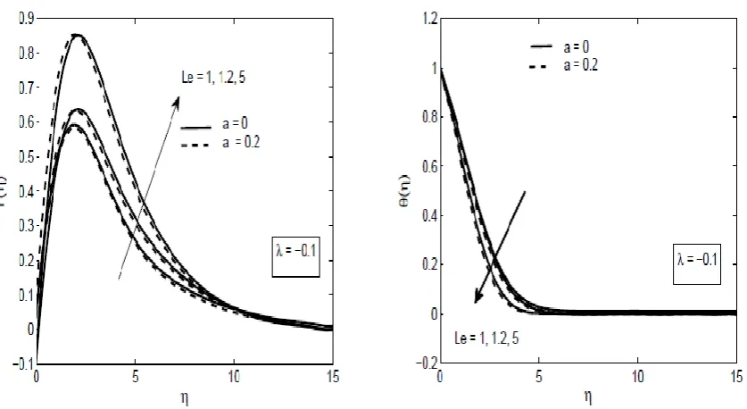
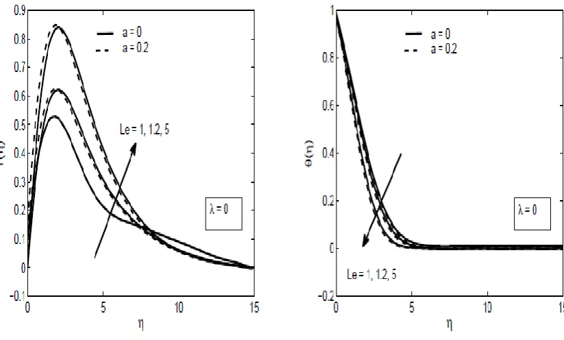
Figures 2-4 depict the effect of sheet stretching/shrinking parameter () and velocity slip

parameter (a) on the dimensionless velocity and temperature. Evidently near the sheet,

increasing velocity slip accelerates the flow velocity inside the boundary layer for a shrinking

sheet (  0.1) and static sheet ( 0) as well as a stretching sheet (0.1). It is further

found that velocity increases for both slip flow and non-slip flow, as the Lewis number

parameter increases. For the conventional no-slip case with sheet-shrinking (a=0, =-0.1),

negative velocities are in fact produced at the sheet and in close proximity to it. The

sheet-shrinking is therefore, in this case, responsible for inducing a significant backflow in the

vicinity of the sheet surface. It is also observed that higher temperatures are achieved for the

no-slip scenario (a=0); and the lowest temperatures correspond to the strong slip case (a=0.2)

for a shrinking sheet ( 0.1) andstatic sheet ( 0) as well as a stretching sheet (0.1

). Thermal boundary layer thickness will therefore be reduced with greater slip effects. Lewis

number is found to decrease the temperature for a shrinking sheet ( 0.1) andstatic sheet (

0 

 ) as well as a stretching sheet (0.1).

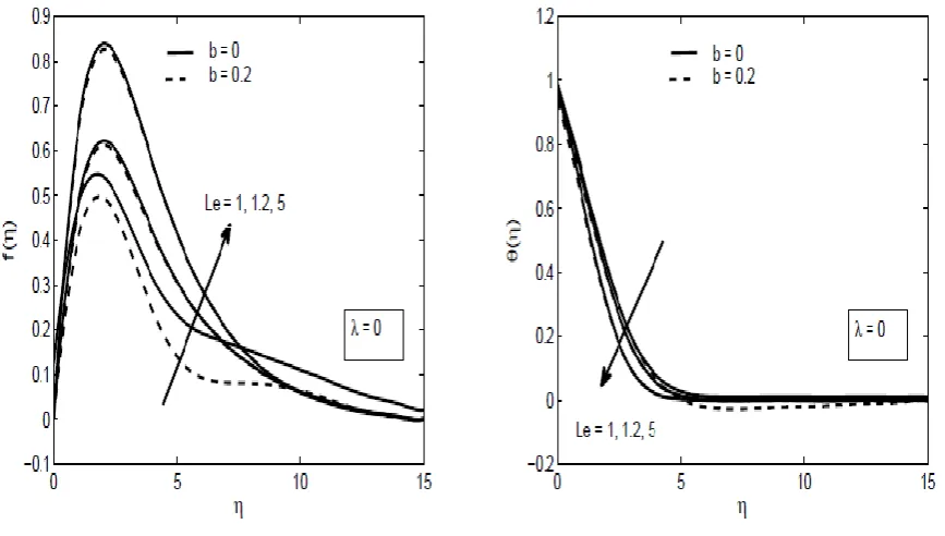
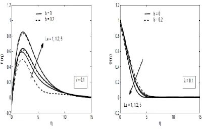
Figures 5-7 depict the effect of the thermal slip and sheet stretching/shrinking parameter ()

on the dimensionless velocity and temperature. It emerges that increasing thermal slip

decelerates the flow inside the boundary layer for a shrinking sheet ( 0.1) and static sheet

( 0) as well as a stretching sheet (0.1). Velocity apparently also increases both in the

presence and absence of thermal slip as the Lewis number rises. Lewis number is directly

proportional to the nanofluid thermal diffusivity and inversely proportional to the nanoparticle

diffusivity. In all the computations presented, Le  0. Both heat and nanoparticle species diffuse

at the same rate for Le = 1 whereas for Le > 1 the heat diffusion rate exceeds the species

flow. There is an intimate connection between the diffusion rate of vorticity (viscosity effect)

and heat and species diffusion. Boundary layer structures (thicknesses) are modified by these

rates. Further, from Figs. 4-6, it is observed that higher temperatures are achieved for the

no-slip scenario (b=0); and the lowest temperature corresponds to the strong thermal slip case

(b=0.2) for a shrinking sheet ( 0.1) andstatic sheet (0) as well as a stretching sheet (

0.1

 ). Thermal boundary layer thickness will therefore be increased with greater thermal slip effects. This has important implications in materials processing since heat control rates at

the wall can be manipulated with wall slip (thermal jump).

Figure 8 depicts the effects of the thermal slip and sheet stretching/shrinking parameter () on

the dimensionless nanoparticle volume fraction. An elevation in thermal slip increases the

nanoparticle concentration for the static sheet (0) as well as a stretching sheet ( 0.1).

However nanoparticle volume fraction decreases for both in the presence of thermal slip and

absence of thermal slip as the Lewis number parameter rises.

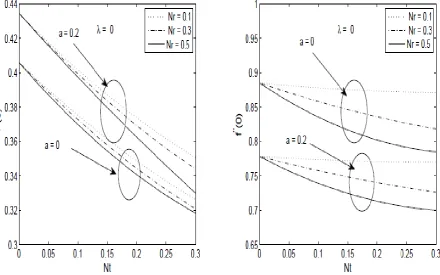
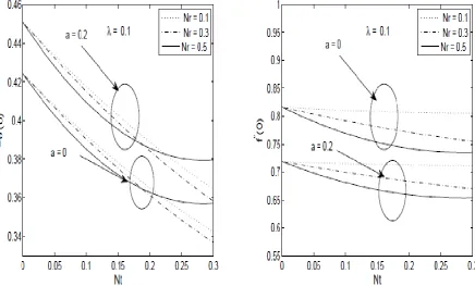
Figures 9-11 depict the effect of the various parameters on the dimensionless friction and the

heat transfer rates. It is observed that the friction is decreased as the thermophoresis parameter

and buoyancy ratio parameter are decreased for both slip flow and conventional no-slip flow.

Friction is decreased as the velocity slip parameter increased. It is further seen from these

figures that heat transfer rate reduces with the thermophoresis and buoyancy ratio parameters

for stretching sheet, stationary sheet and indeed also for a shrinking sheet for both the slip and

no-slip cases. Velocity slip leads to a rise in wall temperature gradient.

5. CONCLUSIONS

Steady-state nanofluid flow from a horizontal plate has been investigated by a combined Lie

group and numerical analysis techniques. Velocity and thermal slip effects, which are of

interest in materials processing operations, have also been incorporated. Passively controlled

boundary condition have been used to attain more robust results. With the aid of a Lie algebraic

group method, the boundary layer equations for momentum, energy and species diffusion

(nanoparticle concentration) have been reduced to a nonlinear, coupled system of ordinary

differential equations. The resulting two-point boundary value problem has been solved

numerically using generalized collocation method. Solutions have been verified with

momentum characteristics have been shown to be controlled by a number of thermophysical

parameters including Brownian motion, thermophoresis, Lewis number, Prandtl number,

velocity slip, thermal slip, buoyancy ratio and sheet stretch/shrink parameter. The present

computations have shown that:

(i) Increasing velocity slip is found to depress temperature and friction whereas it

enhances velocity and heat transfer rates.

(ii) Increasing thermal slip reduces velocity whereas it elevates temperature and

nanoparticle concentration.

(iii) Wall friction is decreased as the thermophoresis parameter and buoyancy ratio

parameter are decreased for both slip flow and conventional no slip flow.

(iv) Heat transfer rates are reduced with the thermophoresis parameter and buoyancy

ratio parameters for stretching, stationary and shrinking sheet cases, for both the

slip and no-slip cases. Velocity slip also leads to a rise in wall temperature gradient.

The present study has been confined to steady flat sheet flow; future studies will consider

transient inclined sheet nanofluid flows, and will be communicated soon.

REFERENCES

Adnan H, Sharma KV, Bakar RA, Kadirgama K, A review of forced convection heat transfer enhancement and hydrodynamic characteristics of a nanofluid, Renew and Sus Ener Rev 29: 734, 2014.

Ali H M, Ali H, Liaquat H, Maqsood HT, Nadir MA, Experimental investigation of convective heat transfer augmentation for car radiator using ZnO water nanofluids, Energy 84:1, 2015

Ascher, Uri M.; Petzold, Linda R, Computer Methods for Ordinary Differential Equations and Differential-Algebraic Equations, Society for Industrial and Applied Mathematics, Philadelphia, USA (1998).

Buongiorno J, Convective transport in nanofluids, ASME J Heat Trans128: 240, 2006.

Choi S, Enhancing thermal conductivity of fluids with nanoparticles, Developments and applications of non-Newtonian flows, D. A. Siginer and H. P., Wang, eds., American Society of Mechanical Engineers, New York, FED- Vol. 231/MD 66: 99,1995.

Coumaressin T, Palaniradja K, Performance analysis of a refrigeration system using nanofluid,

Int J Adv Mec Eng4:459,2014.

Das S K, Choi SUS, Yu W, Pradeep T, Nanofluids: Science and Technology, 1st ed., Wiley, New York, 2007.

Dehghan M, Mahmoudi Y, Valipour MS, Saedodin S, Combined conduction–convection– radiation heat transfer of slip flow inside a micro-channel filled with a porous material, Transp in Porous Med108:413, 2015.

Cantwell, B.J., Introduction to Symmetry Analysis, Cambridge University Press (2003).

Ferdows M, Khan MS, Bég OA, Azad MAK, Alam MM, Numerical study of transient magnetohydrodynamic radiative free convection nanofluid flow from a stretching permeable surface, Proc. IMechE-Part E: J Process Mech Eng 228:181,2014.

Isaacson E, Keller HB, Analysis of Numerical Methods, John Wiley, USA (1966).

Kakac S, Pramuanjaroenkij A, Review of convective heat transfer enhancement with nanofluids, Int J Heat MassTransf52: 3187, 2009.

Karniadakis G, Beskok A, Aluru N, Microflows and Nanoflows Fundamentals and Simulation. In: Microflows and Nanoflows Fundamentals and Simulation. Springer Science, New York, USA (2005).

Kuznetsov AV, Nield DA, Natural convective boundary- layer flow of a nanofluid past a vertical plate, Int J Therm Sci49:243, 2010.

Kuznetsov AV, Nield DA, Natural convective boundary-layer flow of a nanofluid past a vertical plate: A revised model, Int J Ther Sci77:126, 2014.

Mahdi RA, Mohammed HA, Munisamy KM, Saeid NH, Review of convection heat transfer and fluid flow in porous media with nanofluid, Renew and Sus Ener Rev 41:715,2015.

Mauro L, Colangelo G, Milanese M, de Risi A, Review of heat transfer in nanofluids: Conductive, convective and radiative experimental results, Renew and Sus Ener Rev43: 1182, 2015.

Maxwell-Garnett JC, Colours in metal glasses and in metallic films, Philos Trans R Soc London, Ser A, 203:385, 1904.

Minkowycz WJ, Sparrow EM, Abraham JP, Nanoparticle Heat Transfer and Fluid Flow, CRC Press, Boca Raton, Florida, USA (2012).

Murshed SMS, Leong KC, Yang C, Thermophysical Properties of Nanofluids, CRC Press, New York (2011).

Nield DA, Kuznetsov AV, The Cheng-Minkowycz problem for natural convective boundary-layer flow in a porous medium saturated by a nanofluid, Int J Heat Mass Transfer52: 5792, 2009.

Pak BC, Cho Y, Hydrodynamic and heat transfer study of dispersed fluids with submicron metallic oxide particles, Exp Heat Transf 11:151, 1998.

Pradhan K, Samanta S, Guha A, Natural convective boundary layer flow of nanofluids above an isothermal horizontal plate, ASME J. Heat Transf 136:102501, 2014.

Sattler KD, Handbook of Nanophysics: Nanomedicine and Nanorobotics, CRC Press, New York, USA (2010).

Sheikholeslami M, Gorji-Bandpya M, Vajravelu K, Lattice Boltzmann simulation of magnetohydrodynamic natural convection heat transfer of Al2O3–water nanofluid in a horizontal cylindrical enclosure with an inner triangular cylinder, Int J Heat Mass Transf 80:16,2015.

Sonawane S, Bhandarkar U, Puranik B, Kumar SS, Convective heat transfer characterization of aviation turbine fuel-metal oxide nanofluids, AIAA J Thermophy and Heat Transf 26:619, 2012.

Suleimanov BA, Ismailov FS, Veliyev EF, Nanofluid for enhanced oil recovery, J Pet Sci and Eng78: 431, 2011.

Tominaka S, Nishizeko H, Mizuno J, Osaka T, Bendable fuel cells: on-chip fuel cell on a flexible polymer substrate, Energy Environ Sci2:1074,2009.

Vleggaar I, Laminar boundary layer behaviour on continuous, accelerating surfaces, Chem Eng Sci32, 1517, 1977.

Wang BX, Zhou LP, Peng XF, A Fractal model for predicting the effective thermal conductivity of liquid with suspension of nanoparticles, Int J Heat Mass Transfer 46:2665, 2003.

Wang XQ, Mujumdar AS, Heat transfer characteristics of nanofluids: a review, Int J Therm Sci46:1, 2007.

Xuan Y, Li Q, Investigation on convective heat transfer and flow features of nanofluids, ASME J Heat Transf 125:151,2003.

Figure 1: Flow model and coordinate system.

Figure 2: Variation of the velocity distribution f '

 

 

for three values of Le at Pr=6.8, Nr=0.5, Nt=Nb=0.2, b = 0.1 and λ= -0.1.

Figure 3: Variation of the velocity distribution f '

 

 

Figure 4: Variation of the velocity distribution f '

 

 

Figure 5: Variation of the velocity distribution f '

 

 

for three values of Le at Pr = 6.8, Nr = 0.5; Nt = Nb = 0.2, a = 0.1 and λ = -0.1.

Figure 6: Variation of the temperature distribution  

 

 

Figure 7: Variation of the velocity distribution f '

 

 

Figure 8: Variation of the nanoparticle volume fraction distribution  

 

Figure 9. The reduced local Nusselt number and the reduced local skin-friction coefficient relative to thermophoretic parameter for Pr =6.8, Le =5, Nb =0.2 and λ=-0.1.

Figure 10: The reduced local Nusselt number and the reduced local skin-friction coefficient

Figure 11: The reduced local Nusselt number and the reduced local skin-friction coefficient relative to thermophoretic parameter for Pr = 6.8, Le = 5, Nb = 0.2 and λ = -0.1.

Table 1: Values of the reduced skin friction coefficient f ''(0) for Nr=Nt=Nb=0.5, Pr =6.8.

Le

Pradhan et al. (2014) Present work

( 0.1) (0)) (0.1)

5 0.8435 0.8276 0.8435 0.7001

10 0.8806 0.8612 0.8806 0.7506

100 0.9217 0.9106 0.9218 0.7815

Table 2: Values of the reduced Nusselt number '(0)for Nr=Nt=Nb =0.5, Pr = 6.8.

Le

Pradhan et al. (2014) Present work

( 0.1) (0) (0.1)

5 0.3268 0.3142 0.3265 0.3310

10 0.3239 0.3095 0.3238 0.3295