Vertical Upflow Convective Boiling: Flow Regimes, Heat Transfer and EHD Augmentation

Vertical Upflow Convective Boiling: Flow Regimes,

Heat Transfer and EHD Augmentation

Munir Eraghubi

BSc, M Eng

Department of Mechanical and Manufacturing Engineering

Parson Building

Trinity College

Dublin 2

Ireland

A thesis submitted to the University of Dublin in partial fulfilment of the

requirements for the degree of Ph. D

i

Declaration

I declare that I am the author of this thesis and that all work described herein is my own unless otherwise referenced. Furthermore, this work has not been submitted, in whole or part, to any other university or college for any degree or qualification.

I authorize the library of Trinity College Dublin to lend or copy this thesis.

_____________________________

Munir Eraghubi,

ii

Summary

This work is to investigate the effect of electrohydrodynamic force on two-phase flow of HFE7000 refrigerant under convection boiling conditions. The experiment apparatus designed to facilitate the visualization of two-phase flow under EHD field. The test section made of sapphire tube, which allows for optical access to the flow, allows also for heat transfer. A transparent conductive layer of Indium Tin Oxide deposited on the outside surface of the sapphire tube, this (ITO) conductive layer works as sores of heat when connected to an electric power supply. A stainless steel rod runs concentrically along the inside of the sapphire tube and used as the high voltage electrode. The (ITO) layer connected to electrical ground to facilitate EHD force.

The present work is to contribute to the understanding of low quality vertical upflow convective boiling. To this end, measurements are analysed and boiling heat transfer is investigated in the context of boiling curves. Specifically, the influence of mass and heat flux on vertical upward flow are investigated, the results discussed in terms of the observed flow regimes. Finally the heat transfer coefficient results are compared with several existing correlations.

The forced convective boiling experiments with HFE-7000 were conducted for upward flow in a vertical tube at 1.2 bars, inlet subcooling of 2°C and mass flux ranging between 50 and 300 kg/(m2 s).

Initial tests were performed by fixing the flow rate and progressively increasing the heat flux prior to reaching the critical heat flux. A second set of identical tests were performed with a 3 mm diameter stainless steel rod positioned concentrically inside the tube to test the influence of moderate confinement.

iii

Flow regimes for various mass and heat fluxes have been visualized at the central region of the heated section using high speed videography. Three main flow patterns have been observed under different mass and heat fluxes: bubbly flow, bubbly-slug flow and churn flow. The measured boiling conditions were plotted on seven existing vertical flow pattern maps and the agreement discussed.

iv

Acknowledgements

Firstly I want express my deep thanks and admiration to my supervisor Dr. Tony Robinson for all his guidance, patience, enthusiasm, understanding, and endless ideas. I have personal benefited from his knowledge of heat transfer in countless occasions. His ability to define the problems and finding the alternative solutions was amazing. Working with him has been rewarding and a privilege.

I would like to thank Gerry Byrne in the Thermo lab for all his assistance with my modification of the test rig and his problem solving ability. Thanks are due to Mick Reilly, Paul Normoyle, and Workshop staff for their high quality work and Gorgen for his help in Rig design.

I wish also to thank other department staff for their advice help and their contributions in various way including Dr. Tim Persoon, Dr. Seamus O'Shaughnessy, Dr. Tom Lupton, Dr. Nicolas Baudin and Dr. Sajad Alimohammadi.

v

Table of Contents

DECLARATION I

SUMMARY II

ACKNOWLEDGEMENTS IV

TABLE OF CONTENTS V

LIST OF FIGURES X

LIST OF TABLES XVII

NOMENCLATURE XVIII

CHAPTER 1INTRODUCTION 1

1.1 Flow Forced Convective Boiling... 1

1.2 Electrohydrodynamics ... 4

1.3 Scope and Objective ... 6

CHAPTER 2.TWO PHASE FLOW 7 2.1 Basic definitions and terminology ... 7

2.1.1 Confinement number ... 10

2.2 Flow Patterns and Flow Regimes ... 11

2.2.1 Two-phase flow patterns in horizontal tubes ... 12

2.2.2 Two-phase flow patterns in vertical tubes ... 14

2.3 Flow Regime Maps ... 16

2.3.1 Flow Pattern Map for Evaporation in Horizontal Tubes ... 20

2.3.2 Flow Pattern Map in Vertical Tubes ... 22

2.3.3 Effect of tube diameter on flow regime transitions ... 26

2.3.4 Adiabatic and diabatic flow pattern maps ... 27

2.4 Summary of knowledge on flow patterns and regimes ... 29

2.5 Two Phase Flow and Heat Transfer ... 30

2.5.1 Regions of Heat Transfer ... 31

2.6 Flow boiling heat transfer correlation... 33

vi

2.6.2 Shah correlation [71] ... 35

2.6.3 Gungor and Winterton [73] ... 37

2.6.4 Gungor and Winterton [75] ... 37

2.6.5 Jung and Radermacher Correlation [77] ... 38

2.6.6 Kandlikar correlation [66] ... 39

2.6.7 The Wattelet et al. Correlation[65] ... 39

2.7 Summary of knowledge on two Phase Flow and Heat Transfer ... 40

CHAPTER 3.ELECTROHYDRODYNAMIC AUGMENTATION OF HEAT TRANSFER COEFFICIENT 41 3.1 Electrohydrodynamic (EHD) Phenomena ... 41

3.2 Electrohydrodynamic Heat Transfer Augmentation for Horizontal Two-phase Flow 42 3.2.1 Effect of DC Applied Voltage on Heat Transfer Coefficient ... 42

3.2.2 Effect of DC Applied Voltage on Pressure Drop Penalty ... 43

3.2.3 Mass flux effect on EHD augmentation ... 44

3.2.4 Quality effect on EHD augmentation ... 49

3.2.5 Flow Regime Effect on EHD Augmentation ... 51

3.2.6 Electrode Design Effect on EHD Augmentation... 52

3.2.7 Effect of AC Electric Field on EHD Augmentation ... 53

3.2.8 Effect of Low Frequency Applied Voltages Range ... 53

3.2.9 Effect of Intermediate Frequency Applied Voltages Range ... 55

3.2.10 Effect of High Frequency Applied Voltages Range ... 56

3.2.11 Effect of EHD Signal Duty Cycle on HT Performance ... 57

3.2.12 Effect of EHD Signal Modulation on HT Performance ... 58

3.2.13 Effect of EHD Signal Polarity on HT Performance ... 59

3.2.14 Feed back control of Heat Transfer using EHD ... 60

3.2.15 EHD Mechanisms ... 61

vii

3.5 Summary of knowledge on electrohydrodynamic augmentation of heat

transfer coefficient ... 64

CHAPTER 4.EXPERIMENTAL APPARATUS AND METHODOLOGY .... 67

4.1 Experimental Apparatus ... 67

4.1.1 The Primary Loop ... 69

4.1.2 Test Section ... 73

4.1.3 The Electrode and High Voltage Supply ... 81

4.1.4 The Cooling Loop ... 84

4.1.5 Expansion Tank and Refrigerant Reservoir ... 85

4.2 ITO Coated Sapphire Tube ... 85

4.2.1 Thermal Conductivity Considerations of the Sapphire Tube ... 85

4.2.2 Surface Finish of the Tube. ... 87

4.2.3 Variation in thickness of the ITO coating thickness. ... 88

4.2.4 Data acquisition ... 88

4.3 High Speed Imaging System ... 91

4.4 Experimental procedure ... 92

4.4.1 Experimentally Measured Parameters and Test Conditions ... 93

4.5 Data Reduction ... 96

4.5.1 Heat Transfer Coefficient ... 96

4.5.2 Vapour Quality ... 97

4.6 Instrumentation Accuracy and Experimental Uncertainty ... 98

4.6.1 Uncertainty of the heat applied to the test section ... 98

4.6.2 Uncertainty of the Local Heat Transfer Coefficient ... 99

4.6.3 Accuracy of instrumentations ... 100

4.6.4 Experimental Uncertainty ... 100

4.7 Energy Balances ... 102

CHAPTER 5.FLOW VISUALIZATION AND HTC CORRELATION UNDER FIELD FREE CONDITIONS .. 104

5.1 Flow Visualization ... 104

5.2 Comparison to existing flow pattern maps ... 108

viii

5.2.2 Comparison of G-x flow pattern map with Bennett et al. [35] ... 111

5.2.3 Comparison of ρlJl2- ρgJg2 flow pattern map with Hewitt and Roberts [48] 112 5.2.4 Comparison of JL- Jg flow pattern map with Taitel et al. [49], Zhang et al. [51], Ansari et al. [52] and Rozenblit et al. [61] ... 113

5.2.5 Conclusions ... 117

5.3 Heat Transfer under Field Free Conditions ... 118

5.4 Confinement ... 125

5.5 Evaluate boiling convective heat transfer correlation with experimental data 127 5.6 Pool boiling Cooper correlation ... 134

5.7 Conclusions ... 136

CHAPTER 6.EHD ENHANCEMENT OF HEAT TRANSFER . 138 6.1 Heat Transfer under Field Free Conditions ... 139

6.2 AC EHD Augmentation ... 141

6.2.1 Influence of 100 Hz EHD on flow regimes and heat transfer ... 147

6.2.2 Bubble generation at the wall ... 149

6.2.3 Bubble motion in the core flow ... 151

6.3 Influence of applied voltage frequency for low heat flux ... 153

6.3.1 Flow regime at 1 Hz ... 154

6.3.2 Flow regime at 10 Hz ... 162

6.3.3 Flow regime at 60 Hz ... 165

6.4 Frequency effect at higher heat flux ... 167

6.5 Conclusion ... 172

CHAPTER 7. CONCLUSIONS AND FUTURE WORK 175 7.1 Future Work ... 178

REFERENCES 179 APPENDICES 187 Appendix A. Pre-Heater Power Requirement ... 187

ix

Appendix C: Optical Transmission Qualities of ITO coating ... 190

Appendix D Refrigerant HFE7000 properties ... 191

Appendix E Combined Convection and Radiation losses from Test Section ... 194

x

List of Figures

Figure ‎1-1. View of the experimental heat pipe payload onboard MIOSat [9] ... 2

Figure ‎1-2. New thermal management concept for a smartphone equipped with a loop heat pipe [10] ... 2

Figure ‎1-3. Heat pipes built on P35 Express motherboards [11] ... 3

Figure ‎1-4. The mission patch for the planned test of the EHD pump aboard the International Space Station.(Source: WPI) [20] ... 5

Figure ‎1-5. Schematics of the EHD printing systems with position synchronization [21] ... 5

Figure ‎2-1. Flow regimes in horizontal, condensing two-phase flow [30] ... 13

Figure ‎2-2. Schematic of flow patterns in vertical upward gas liquid flow [35] ... 15

Figure ‎2-3. Baker flow map for horizontal tube [30] ... 16

Figure ‎2-4. Flow pattern map for gas-liquid in horizontal pipes [38] ... 17

Figure ‎2-5. Taitel and Duckler [39] Two phase flow Pattern map for horizontal tube19 Figure ‎2-6. Kattan et al. [40], 23] flow pattern map (S : stratified, SW : stratified-Wavy, I : intermittent, A : annular, M : mist flow) ... 20

Figure ‎2-7. Thome-El Hajal [43] flow pattern map for refrigerant R-22 ... 21

Figure ‎2-8. Wojtan-Ursenbacher-Thome [44] flow pattern map... 22

Figure ‎2-9. Two phase flow pattern map of Fair for vertical tubes [45] ... 22

Figure ‎2-10. Bennett et al. [46] Flow pattern for steam-water flow in 12.7 mm bore tube at 6.89 MPa [46] ... 23

Figure ‎2-11. Vertical upward flow regime map of Hewitt and Roberts [48] ... 24

Figure ‎2-12. Taitel et al. (1980) flow pattern map for vertical flow [49] ... 25

Figure ‎2-13. Flow pattern map for water/air in 82.6 mm diameter tube, by Zhang et al [51]. ... 25

Figure ‎2-14. Flow pattern maps for upward gas–liquid two-phase ... 26

Figure ‎2-15. Forced convective boiling with qualitative temperature profile for a uniform heat flux boundary condition [31]... 32

xi

Figure ‎3-2. Effect of varying the varying applied voltage on the pressure drop at G = 83.4

kg/(m2 s), q”= 10.2 kW/ m2 , xin = 66% [83] ... 44 Figure ‎3-3. The effect of mass flux on the average condensation heat transfer coefficients,

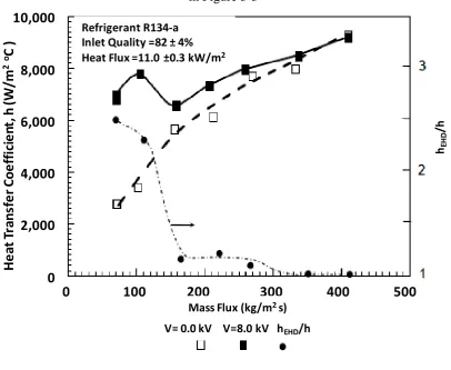
for applied voltages of 0 kV and 8 kV DC [86]. ... 45 Figure ‎3-4. The effect of mass flux on heat transfer,  0 kV, Δ EHD 8 kV, q” = 5.7 kW/m2

, xavg = 45% [6] ... 46

Figure ‎3-5. The relationship between ratio as a function of current at 24 ˚C [88] ... 47 Figure ‎3-6. Experimental relationship between the ( ) ratio as a function of applied

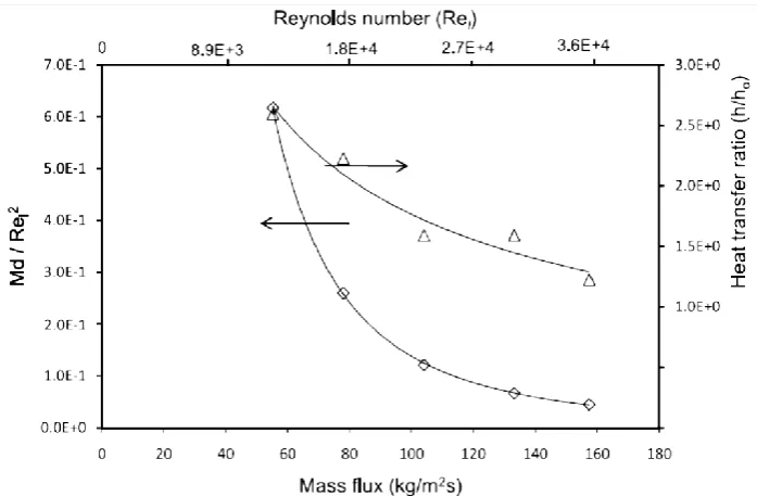
voltage at 24 ˚C [88] ... 48 Figure ‎3-7. The effect of mass flux on ◊ ( ), and Δ (hEHD/ho) at (8 kV), q”= 5.7 kW/m2

and xavg = 45% [16] ... 49 Figure ‎3-8. The effect of inlet quality on condensation heat transfer coefficients and, for

applied voltages of 0 kV and 8 kV DC [86] ... 50

Figure ‎3-9. Heat transfer coefficient and pressure drop versus change in quality at Gavg=99.9

kg/(m2 s) and Tsat at 4.9°C [82] ... 51

Figure ‎3-10. Heat transfer coefficient without EHD forces for experimental-bottom,

experimental-top,  model-bottom, Δ model-top [16] ... 52 Figure ‎3-11. The Effect of the DC and AC Masuda numbers on the average Nusselt number

[18] ... 53 Figure ‎3-12. Effect of frequency (Hz) on heat transfer enhancement ratio. Measurements

taken for square a wave between 0kV and 8 kV and constant mass flux of G= 55 kg/(m2 s), inlet quality (x= 45%) and outlet quality (x=30%) [96] ... 54

Figure ‎3-13. Effect of pulse repetition rate on pressure drop ratio G = 57 kg/(m2 s, G = 100 kg/(m2 s, G = 150 kg/(m2 s) [95] ... 55

Figure ‎3-14. Effect of pulse repetition rate on heat transfer ratio. G = 57 kg/(m2 s, G = 100 kg/(m2 s, G = 150 kg/(m2 s) [95] ... 56

Figure ‎3-15. Local Heat Transfer Coefficients along the Top Portion of the Tube [18]57 Figure ‎3-16. The effect of pulse repetition rate on heat transfer, 25%, 50%, 75% duty

xii

Figure ‎3-17. Effect of duty cycle on heat transfer enhancement ratio. Pulse width 58 ms, xavg

50%, G of Δ45, □55, and ○ 110 kg/(m2 s) [90]... 58

Figure ‎3-18. Effect of duty cycle on the heat transfer enhancement ratio for a mass flux of 55 kg/(m2 s), xav of 50% and pulse width of ○ 29, Δ58, and □ 115 ms ... 59

Figure ‎3-19. Heat transfer enhancement versus pressure drop penalty for EHD waveform parametric study. G = 60 kg/(m2 s, xav= 40%, q" = 7.5 kW/m2[94] ... 60

Figure ‎3-20. Heat transfer coefficient profiles at the entrance of the tube, G = 100 kg/(m2 s), q”= 12.4 kW/m2, P = 1 atm ... 65

Figure ‎4-1. Schematic representation of the rig ... 69

Figure ‎4-2. New pre heater design ... 70

Figure ‎4-3. Test section 3D diagram ... 75

Figure ‎4-4. Polypropylene supports, O-rings seal and seal cap ... 76

Figure ‎4-5. Schematic representation of the test section ... 77

Figure ‎4-6. Test section showing developing length, sapphire tube and polypropylene support pieces ... 78

Figure ‎4-7. Type-T thermocouple with sealing gland ... 79

Figure ‎4-8. Test section, conductive clamps and thermocouples position ... 80

Figure ‎4-9. Tripod spacers support ... 81

Figure ‎4-10. Conductive clamp ... 82

Figure ‎4-11. Electrical schematic of the test section... 83

Figure ‎4-12 Two ungrounded T type thermocouple imbedded into into the wall of the sapphire tube ... 84

Figure ‎4-13. Biot Number for boiling conditions ... 86

Figure ‎4-14. WLI image of the sapphire tube ... 88

Figure ‎4-15. Data logging hardware ... 89

Figure ‎4-16. Front panel of Labview® data acquisition program ... 91

Figure ‎4-17. Energy balance on the preheater ... 102

Figure ‎4-18. Condenser energy balance ... 103

Figure ‎5-1. Different flow regimes and how they are identified ... 105

xiii

Figure ‎5-3. Flow regime cartoon (a) Partial nucleate boiling(b) fully bubbly flow (c) Slug flow

(d) Churn flow (e) Transitional to annular flow ... 107

Figure ‎5-4. Flow visualisation at q//=36 kW/m2 for different mass fluxes (a) 50 kg/(m2 s)(b) 150 kg/(m2 s) (c) 300 kg/(m2 s) ... 108

Figure ‎5-5. Comparison of G -1/Xtt flow pattern map with Fair [26]. ... 110

Figure ‎5-6. Comparison of G-x flow pattern map with Bennett et al. [44] ... 112

Figure ‎5-7. Comparison of ρlJl2- ρgJg2 flow pattern map Hewitt and Roberts [48] .... 113

Figure ‎5-8 Comparison of JL- Jg flow pattern map with air/water Taitel et al. [49] map114 Figure ‎5-9. Comparison of JL- Jg flow pattern map with calculated air/water Taitel et al. [49] map ... 115

Figure ‎5-10. Comparison of JL- Jg flow pattern map with Zhang et al. [51] ... 115

Figure ‎5-11. Comparison of JL- Jg flow pattern map with Ansari et al. [52] ... 116

Figure ‎5-12. Comparison of JL- Jg flow pattern map with Rozenblit et al. [61] ... 117

Figure ‎5-13. Boiling curve at 100 kg/(m2 s) , ΔTsub=2°C ... 120

Figure ‎5-14. Heat transfer coefficient versus heat flux at 100 kg/(m2 s), ΔTsub=2°C . 121 Figure ‎5-15. Heat transfer coefficient vs heat flux for two different mass fluxes. .... 124

Figure ‎5-16. Compare between the circular flow and the annular flow (a) Re =2100, (b) Re=3050 ... 126

Figure ‎5-17. (a), (b) 100 kg/(m2 s), 10 kW/m2 (c), (d) 150 kg/(m2 s), 35 kW/m2,(e) , (f)100 kg/(m2 s), 60 kW/m2 [(a), (c), (e) unconfined flow, (b), (d), (f) semi-confined flow] ... 127

Figure ‎5-18. Measured HTC vs Chen correlation [67] ... 129

Figure ‎5-19. Measured HTC vs Shah correlation [71] ... 130

Figure ‎5-20. Measured HTC vs Gungor & Winterton [73] ... 131

Figure ‎5-21. Measured HTC vs Wattelet et al. correlation [65]... 131

Figure ‎5-22. Measured HTC vs Jung & Radermacher [77] ... 132

Figure ‎5-23. Measured HTC vs Gungor & Winterton [75] ... 133

Figure ‎5-24. Measured HTC vs Kandlikar [66]... 133

Figure ‎5-25. Measured data vs Wattelet et al. [65] and Shah [71] errors ... 134

xiv

Figure ‎6-1. Free field boiling heat transfer coefficients vs heat flux. Retest for G=100 kg/(m2

s). Tubular ... 140 Figure ‎6-2. Field free flow regime a (a) 6 kW/m2 (b) 16 kW/m2 ... 141 Figure ‎6-3. HTC and the enhancement at G=100 kg/(m2 s), q//=6 kW/m2 and V=0- 8 kVp-p

@100 Hz (a) HTC vs voltage magnitude, (b) HTC enhancement vs voltage magnitude

... 142 Figure ‎6-4. HTC and the enhancement at G=100 kg/(m2 s), q//=16 kW/m2 and V=0- 10 kVp-p

@100 Hz (a) HTC vs voltage magnitude, (b) HTC enhancement vs voltage magnitude

... 143 Figure ‎6-5. HTC and the enhancement at G=100 kg/ (m2 s), q//=6 kW/m2 and 16 kW/m2 and

V=0- 10 kVp-p @100 Hz (a) HTC vs voltage magnitude, (b) HTC enhancement vs voltage

magnitude ... 146 Figure ‎6-6. Flow visualization for 0 kV (left) and 8 kV (right) at 100Hz, (a) 6 kW/m2 (b) 16

kW/m2 ... 147

Figure ‎6-7. Observed flow regimes at different EHD voltage G=100 kg/(m2 s), q//= 16 kW/m2,

f=100 Hz, V=0-8 kV AC (a) 0 kV (b) 2 kV (c) 4 kV (d) 6 kV (e) 8 kV ... 148

Figure ‎6-8. Bubble size (a) under free field condition (b) under 8 kV for G=100 kg/(m2 s), q//=

16 kW/m2, f=100 Hz ... 149

Figure ‎6-9. Bubble growth time under free field condition q//= 16 kW/m2 (a) 0 second Frame

1 (b) 30 ms Frame 30 ... 150 Figure ‎6-10. Bubble growth time under 8 kV 100 Hz (a) Frame at 0 ms (b) Frame 30 at 30 ms

... 150 Figure ‎6-11. Bubbles Zigzagging under EHD forces ... 151 Figure ‎6-12. (a) HTC vs the frequency, (b) HTC enhancement vs frequency for G=100 kg/(m2

s), q//=6 kW/m2, V=10 kVp-p and f=1 - 1000 Hz ... 153

Figure ‎6-13. Over all test section images G=100 kg/(m2 s), q//=6 kW/m2 , V=10 kVp-p (a) 1 Hz

(b) 10 Hz (c) 60 Hz ... 154

Figure ‎6-14. Voltage and flow regime cycles for G=100 kg/(m2 s), q//=6 kW/m2 , V=10 kVp-p at

xv

Figure ‎6-15. Schematic of Transition (T) phase where charge injection from the wall into the

fluid negatively charges the bubbles (top) causing them to be attracted to the positive electrode (bottom) ... 158 Figure ‎6-16. Schematic of Vapour Contraction (VC) phase where all of the vapour has been

attracted to the electrode and is held there as it discharges ... 159 Figure ‎6-17. Schematic of Churn (VC) phase where the discharged vapour has been forced

back into the bulk flow and is acted on by the dielectrophoretic force pushing it towards the wall (top) causing a well-mixed churn flow (bottom) ... 160

Figure ‎6-18. Percentage time for each flow regime at 1 Hz, 10 kV p-p ... 161

Figure ‎6-19. Voltage and flow regime cycles for G=100 kg/(m2 s), q//=6 kW/m2 , V=10 kVp-p at

10 Hz ... 163 Figure ‎6-20. Percentage time for each flow regime at 10 Hz, 10 kV p-p ... 164

Figure ‎6-21. Voltage and flow regime cycles for G=100 kg/(m2 s), q//=6 kW/m2 , V=10 kVp-p at

100 Hz ... 166 Figure ‎6-22. Percentage time for each flow regime at 60 Hz, 10 kV p-p ... 167 Figure ‎6-23. (a) HTC vs the frequency, (b) HTC enhancement vs frequency for G=100 kg/(m2

s), q//=16 kW/m2 , V=10 kVp-p and f=1 - 1000 Hz ... 167

Figure ‎6-24. Comparing high and low heat flux Results (a) HTC vs the frequency (b) HTC

enhancement vs frequency... 168

Figure ‎6-25. Over all test section images 100 kg/(m2 s), 10 kV, 16 kW/m2. (a) 10 Hz (b) 60 Hz

(c) 100 Hz (d) 500 Hz ... 169

Figure ‎6-26. Voltage and flow regime cycles for G=100 kg/(m2 s), q//=16 kW/m2 , V=10 kVp-p at

10 Hz ... 171 Figure ‎6-27. Percentage time for each flow regime at 10 Hz, 10 kVp-p, 16 kW/m2 k 172

Figure ‎7-1. Optical transmissibility of Diamox ITO coating at 300Ώ/m2 ... 190 Figure ‎7-2. Variation of Density of HFE7000 with temperature ... 191 Figure ‎7-3. Variation of specific heat of HFE7000 with temperature ... 191 Figure ‎7-4. Variation of latent heat of vaporisation of HFE7000 with temperature . 192 Figure ‎7-5. Variation of dynamic viscosity against temperature for water, source [124]

xvi

Figure ‎7-7. Variation of Density viscosity against temperature for water, source [112]193 Figure ‎7-8. Heat input vs. (A. ΔT) for determining the combined convection radiation heat

xvii

List of Tables

Table ‎2-1. Macro to micro-channel transition limits ... 10

Table ‎2-2. Adiabatic experimental studies for vertical flow pattern maps ... 28

Table ‎2-3. Vapour/liquid experimental studies for flow pattern maps ... 29

Table ‎2-4. Nucleate boiling heat transfer coefficient correlations for the Shah correlation. ... 36

Table ‎4-1. Properties of HFE7000 @ 25°C (from 3M Corp) [111]... 68

Table ‎4-2. Summary of Fluid Properties Determined from Temperature and pressure90 Table ‎4-3. Summary of Experimental Conditions in Test Section ... 94

Table ‎4-4. Experimental Measurements ... 95

Table ‎4-5. Accuracy of instrumentation. ... 100

Table ‎4-6. The relative uncertainty in heat transfer ... 100

Table ‎4-7. The relative uncertainty in the heat transfer coefficient ... 101

Table ‎5-1. Observed Flow-Pattern Data Against Predicted Flow Pattern Flow-Pattern Maps. ... 109

Table ‎5-2. Comparison between experimental data and correlation predictions. ... 128

Table ‎6-1. Varied Parameters for each test ... 139

Table ‎7-1. maximum and minimum power required for pre heater ... 187

Table ‎7-2. Pre heater electrical resistance... 188

xviii

Nomenclature

Latin Symbols

Symbols Name Units

A area m2

Bi Biot number -

Bo Boiling number -

Cp specific heat J/(kg K)

Co Convection number -

d test section diameter m

Dh hydraulic diameter m

f friction factor -

F Convective enhancement factor -

Fr Froude number -

E Electric field strength V/m

G mass flux kg/(m2 s)

g Gravity and Acceleration m/s2

hfg latent heat J/ kg

I current A

J superficial velocity m/s

k thermal conductivity W/(m K)

K parameter in Taitel and Duckler map -

h heat transfer coefficient W/(m2 K)

mass flow rate kg/s

Md Masuda number -

Nu Nusselt number -

P pressure Pa

Re Reynolds number -

q” heat flux W/m2

qL natural convection losses W/m2

S Suppression factor -

xix

T Temperature °C

T parameter in Taitel and Duckler map -

V voltage V

u_ Phase velocity m/s

x quality (dryness fraction) -

Xtt Lockart-Martinelli parameter -

Greek symbols

α void fraction -

ε_ Dielectric permittivity F/m

gas-phase parameter, Baker flow map -

μ dynamic viscosity kg/m.s

ρ density kg/m3

σ surface tension, N/m

ν kinematic viscosity m2/s-

liquid-phase parameter, Baker flow map -

Friction Multipliers -

Subscripts Subscipts

Cb convection boiling

G gas

i inner

l liquid

nb nucleate boiling

o outer

sat saturation

sup superheat temperature

tp two phase

v vapour

1

Chapter 1.

Introduction

1.1

Flow Forced Convective Boiling

Flow boiling is a very effective technique for removing large amounts of heat at a targeted temperatures for a given mass flow rate of coolant due to the large latent heat of vaporization, the high heat transfer coefficients and relatively small inlet-to-outlet temperature differences compared to the single-phase flow [1]. Due to these and other reasons, forced boiling systems are broadly used in various industrial applications and very common in everyday life, including central heating, air conditioning, thermal power plants, nuclear reactors, water-cooled gas turbines, internal combustion engines, X-ray sources [2] [3], to name a few.

Flow boiling heat transfer is also used in space platforms and satellites design [4], where very efficient, compact and lightweight devices are required [5] [6]. Heat pipes, for example are used to transport heat from inside to outside the spacecrafts and satellites, and do not require gravity to operate. Figure ‎1-1 shows an experimental heat pipe payload onboard MIOSat.

2

Figure ‎1-1. View of the experimental heat pipe payload onboard MIOSat [9]

3

Figure ‎1-3. Heat pipes built on P35 Express motherboards [11]

Flow boiling describes the boiling of flowing liquids along superheated surfaces whereby there is sufficient heat transfer to the fluid to cause vaporization. Generally, heat is transferred in flow boiling by either vaporization or nucleate boiling. For the later, formation, growth and detachment of discrete vapour bubbles on the superheated surface defines nucleate boiling-based flow boiling regimes. Conduction and convection through a liquid film in contact with the superheated surface with subsequent vaporization at the two-phase interface defines vaporization-based convective boiling regimes [12].

4

In the high quality regions, forced convection is the main heat transfer mechanism with nucleate boiling being usually suppressed at qualities higher than 0.2. In this region the corresponding flow pattern is annular flow, wherethe heat is transferred by the conduction and convection modes across the liquid film while the evaporation takes place at the interface between the liquid and the vapour. The heat transfer coefficient is less dependent on the heat flux and tends to increase with the increase in mass velocity and vapour quality [14].

1.2

Electrohydrodynamics

Electrohydrodynamics (EHD) involves the application of intense electric fields to fluids. In two phase flow, electrostatic body forces can be large enough to change the flow regimes in such way to enhance the heat transfer. This allows for the opportunity for making heat exchangers more effective and compact as well as intelligent.

This project will study the two-phase flow behaviour in tubular heat exchangers with the aim of understanding the influence of Electrohydrodynamics on local heat transfer coefficient.

Electrohydrodynamics (EHD) is the branch of thermal fluid science that deals with the interaction of high-voltage electric fields with fluids. This interaction induces electric body forces within the fluid, which can affect the two-phase flow, and therefore heat transfer and pressure drop [15] [16].

Heat transfer enhancement improves the performance of the heat exchanger and at the same time enables a considerable decrease in size, weight, volume, material and costs.

The field of EHD heat transfer enhancement has been continuously studied over the past 70 years. The earlier work was more concentrated on the enhancement of single-phase flow. In the last 30 years, many studies and researchers have shown a greater potential of EHD in enhancing two-phase heat transfer.[17]

5

EHD is that the heat transfer may be enhanced without a significant increase in pressure drop [16][18]. As such, EHD may allow for the production of highly compact and low cost heat exchangers with the possibility of solid state control.

A wide range of applications for EHD are reported in the literature e.g. pumping, single phase heat transfer, boiling, condensation, mixing, and liquid jets, (see Figure ‎1-4 and Figure ‎1-5) [19] [20] [21].

Figure ‎1-4. The mission patch for the planned test of the EHD pump aboard the International Space Station.(Source: WPI) [20]

Figure ‎1-5. Schematics of the EHD printing systems with position synchronization

6

The typical value of the current required to enhance the heat transfer associated with EHD is very low, resulting in very small power consumption comparing with other traditional technologies. This makes EHD an ideal method for heat transfer augmentation in microgravity [22].

1.3

Scope and Objective

The overarching objective of this research is to investigate vertical upflow boiling both with and without the effect of EHD. Specifically, a test facility will be constructed to allow the simultaneous observation of the vertical two phase flow and the measurement of the local heat transfer coefficient. Thus, the first sub-objective of this work is to study the flow regimes of vertical upflow boiling for varying heat and mass flux conditions. The results will be compared with existing flow regime maps which were developed for isothermal air-water systems or those developed in adiabatic viewing sections. In a similar way, the second sub-objective will involve the measurement of the heat transfer coefficient for vertical upflow boiling with the unique capacity to observe the flow regime where the measurements will be taken. Thus, the heat transfer will be related to changes in the flow boiling conditions for different heat and mass flux levels. Finally, the influence of EHD on the flow and heat transfer will be investigated. This will focus on the lower quality bubbly flow regime and the influence of high voltage magnitude and frequency on the two phase flow and heat transfer will be studied. Once again, the transparent yet diabatic test section will allow any changes in the heat transfer to be related to the flow dynamics.

7

Chapter 2.

Two Phase Flow

Multiphase flow is the simultaneous flow of two or more phases separated from each other by distinct interfaces. One common case of multiphase flow is two-phase flow, where at least one of the phases is a liquid, and the other is vapour or gas [23]

Two-phase flow has been applied to many fields because of its higher energy efficiency in comparison with single-phase flow, because of lower pumping power and higher heat transfer coefficients. Practical examples of gas-liquid flows take place in several applications such as: the flow of oil and gas in oil pipelines, the flow of steam and water in power plants and in steam-heating pipes and the flow of liquid and vapour refrigerants in the condensers and evaporators of refrigeration and air conditioning equipment.

In this work, the focus is on two-phase flows in which a liquid and vapour flow together in a straight tube, which is a very common scenario in heat transfer applications.

2.1

Basic definitions and terminology

This section defines the important parameters that are used to characterize the heat and mass transfer of two phase flows and is included here as they will be used throughout the manuscript.

The total mass flow rate ( ) is the sum of the mass flow rate of liquid phase ( ) and the vapour phase ( ):

8

The total mass flux of the flow (G) is defined the total mass flow rate ( ) divided by the cross-sectional area of the flow (A),

₍₂₎

The quality (dryness fraction), x, is defined as the ratio of the mass flow rate of vapour phase ( ) to the total mass flow rate ( ),

(3)

The void fraction ( ) is defined here as the ratio of the cross-sectional area occupied by the vapour phase ( to the total cross-sectional area (A) of the flow.

₍₄₎

The phase velocity is the volume flux divided by the cross-sectional area occupied by the phase.

(5)

(6)

The slip ratio is defined as the ratio of the vapour and liquid phase velocities,

(7)

(8)

9

(9)

(10)

The Reynolds number for vapour and liquid are thus defined as:

(11)

(12)

The Froude number (Fr) represents the ratio of inertial forces to gravitational forces and is defined as:

(13)

The Froude gas number for the vapour phase is defined as:

₍₁₄₎

For the liquid phase, the Froude number can be expressed as:

(15)

The Martinelli parameter, X, is a ratio of pressure drops of the single-phase flow terms and is defined as:

(16)

10

₍₁₇₎

The Masuda number (Md), or dielectric Rayleigh number is defined as:

(18)

Where is the fluid permittivity, E is the electric field strength, is the fluid density and T is the fluid temperature, dielectric constant.

It represents the relative strength of the electric field to that of viscosity and sometimes referred to as the Electric Rayleigh number.

2.1.1 Confinement number

The heat transfer and flow characteristics can be different over the ranges of millimeter to sub-millimeter size, and over the years, there has been much debate about what identifies a channel size as conventional or miniature. Mehedale et al. [24] and Kandlikar et al. [25] distinguish micro-channels from macro-channels based on the characteristics of channel size. Mehendale et al. [24] used the term meso-scale which is in between the micro and macro-scales whereas Kandlikar et al. [25] used the term mini-channel for a larger range, see Table ‎2-1

Table ‎2-1. Macro to micro-channel transition limits

Channel Mehendale et al. [24]

D

Kandlikar et al. [25]

D

Micro-Channel 1-100 μm 10-200 μm

Meso-Channel 100-1000 μm

Mini-Channel 200 μm-3 mm

Macro-Channel 1-6 mm

Conventional Channel > 6 mm > 3 mm

11

size of the channel that defines the shift from isolated bubble regime to confined bubble regime and subsequently from large tubes to micro-channels based on physical criterion [26]. The Confinement Number was defined by Cornwell and Kew [23] in terms of the capillary number and the channel hydraulic diameter such that,

(19)

Many studies of flow and heat transfer under a variety of conditions suggests that a broad general rule is that for Co> 0.5, confined bubble flow occurs and the effects of confinement will be significant [27]. Ong and Thome [28] described a transition region between micro and macro scale flow behaviour, referred to as meso-scale, using Co. It was found that this transition regime was present for 0.3 < Co < 0.4. Conventional unconfined channel flow is expected for Co < 0.3.

In the case considered here, for the flow regime and heat transfer coefficient tests, the flow is in an 8 mm circular tube, which is classified as conventional macro-scale flow. For the EHD test where an electrode was inserted inside the tube, Dh found 2.5 mm, which considered as a meso-scale channel.

2.2

Flow Patterns and Flow Regimes

Many types of liquid and vapour phase distributions can occur when two phase mixtures flow in a channel. This is commonly referred to as flow patterns or flow regimes. The type of flow pattern depends on the size and orientation of the flow channel, the difference between the vapour and liquid flow parameters, the gravitational forces acting on the flow, and the fluid properties.[29]

12

The flow regimes in vertical and inclined tubes are considerably different from those in horizontal tubes. The focus in this work is exclusively for the two phase flow regimes in horizontal and vertical tubes only.

2.2.1 Two-phase flow patterns in horizontal tubes

13

Figure ‎2-1. Flow regimes in horizontal, condensing two-phase flow [30]

From Figure ‎2-1 the flow regimes can be divided into two broad groups: in the top five regimes, the vapour flows as a continuous stream, in the bottom three types the vapour fragments are separated from each other by liquid. The flow regime is significantly influenced by the void fraction and the vapour flow rate. Generally, the vapour flow as a continuous stream if the void fractions is greater than 0.5.

14

As the vapour flow rate is increased further, the liquid starts to climb the side tube wall. When the tube wall is wetted completely by liquid, the flow pattern is described as annular flow, where a liquid layer flows along the wall and vapour flows in the core. Annular-mist flow takes place when a high vapour flow rates causes agitation of liquid at the interface, and this liquid becomes entrained in the vapour flow in the form of fine droplets.

In case of low void fraction, the vapour may cause rising columns of liquid to reach the top of the tube and break the continuity of vapour stream. These liquid columns are called a "slugs" and a flow of this pattern is called slug flow. Plug flow can be realized at lower void fractions, when the vapour becomes completely enclosed in the liquid in a form of elongated bubbles. Further lowering the void fraction results in smaller vapour bubbles travelling with the liquid stream, called bubbly flow [30].

2.2.2 Two-phase flow patterns in vertical tubes

When the flow is oriented upward in a vertical tube, gravity acts parallel to the flow resulting in notable differences in the two phase flow structures compared with the horizontal configuration. These are depicted in Figure ‎2-2 and are described as follow:

Bubbly flow: Small bubbles are dispersed as distinct substances in the liquid continuum flow. Distinctive features of this flow are moving and deformable of shapes but they are typically spherical and much smaller than the tube diameter, as shown in Figure ‎2-2.

15

Churn Flow: Churn flow is one of the least understood of gas-liquid flow regimes, and it appears only in vertical and near-vertical channels when there is a large gas fraction with a high velocity and small liquid fraction with low velocity. The flow regime is highly disturbed flow of gas and liquid and is distinguished by the presence of a very thick and unstable liquid film with the liquid often oscillating up and down. It is usually bounded by the slug and the annular flow regimes. Recent evidence suggests that Slug Flow is destabilized when the liquid film surrounding a Taylor bubble is flooded by the gas flowing upwards [33].

Annular Flow: With a higher gas velocity and a void fraction above 75-80%, the interfacial shear becomes dominantover gravity and the liquid is expelled from the centre of the tube and flows as a thin film on the channel wall, while the gas flows in the core of the tube. Annular flow can be pure or dispersed flow depending on the fraction of entrained small liquid droplets contained in the core gas flow.[34]

Figure ‎2-2. Schematic of flow patterns in vertical upward gas liquid flow [35]

Wispy-Annular: At relatively higher gas flow rates, the entrained droplet may form a coherent structure as clouds or wisps of fluid. This flow pattern was first identified by Bennett et al. [36], but not observed in many studies. [37]

16

2.3

Flow Regime Maps

The observations of the flow regimes are usually plotted on a graph, the axes representing the flow rates of each phase flow, though in some instances the total mass flux of the two phases is represented on one axis and the other axis representing the mass fraction of the flow or vapour quality. Lines are incorporated between the various flow regimes on the graphs to represent the boundaries between each flow pattern to produce a “flow regime map”.

In 1954, Baker correlated the flow regime to the volume flow rates of the vapour and the liquid and proposed one of the first flow regime maps as depicted in Figure ‎2-3.

Figure ‎2-3. Baker flow map for horizontal tube [30]

The axes are defined in terms of Gg/ and G_l , where the gas-phase parameter is

defined as:

(20)

17

(21)

Based on several studies and observations, Mandhane et al. [38] proposed the flow regime map shown in Figure ‎2-4. The flow pattern map coordinates are determined by the superficial liquid and vapour flux ( , ) (see Equations (9), (10)). The superficial velocity of the vapour jv represents the horizontal coordinate, the superficial velocity of the liquid jl represents the vertical coordinate. Figure ‎2-4 shows that at higher liquid flow rates, the flow has either slugs or bubbles and increasing the vapour superficial velocity results in an annular flow regime.

Figure ‎2-4. Flow pattern map for gas-liquid in horizontal pipes [38]

In practical applications a more general flow regime map is usually needed. These means that more data from a variety of fluids and a wider range of tube diameters must be included in the map. For this purpose, reasonable dimensionless groups have to be selected to represent these varying parameters.

jgm.s-1

jl

m.

s-1

bubbly

slug

stratified plug

annular

18

Taitel and Duckler [39] suggest that in order to find appropriate dimensionless groups for the coordinates on flow regime maps, the mechanisms that lead to the flow regimes must be understood. They proposed four dimensionless groups to describe the flow regimes; the Martinelli parameter Xtt, the gas Froude number FrG, and new parameters K and T. Using these parameter they developed a three-part map shown in Figure ‎2-5, with parameter FrG and X defined in Equations (14) and (22) respectively.

(22)

Taitel and Duckler defined the K parameter as:

(23)

They also defined the parameter T as:

(24)

The pressure gradient in equation (24) for the liquid phase is given by:

₍₂₅₎

The friction factor in the above equation depends on the flow Reynolds number. If Re <2000, the laminar flow calculation is used:

(26)

If Re > 2000, the friction factor is calculated by the turbulent correlation,

19

To determine the type of the flow using the Taitel and Duckler [39] map, first the X and FrG are calculated and plotted on the top graph. If the coordinates (X, FrG) fall in annular flow area, then the type of flow is annular. If the coordinates (X, FrG)fall in the lower left area, then K is calculated and the flow regime is identified using the middle graph. If the coordinates (X, FrG) fall in the lower right area, then T is calculated and the flow regime identified using the bottom graph.

Though the Taitel and Duckler flow pattern maps were developed for adiabatic two-phase flows, they are often used with diabatic processes of evaporation or condensation.

20

2.3.1 Flow Pattern Map for Evaporation in Horizontal Tubes

2.3.1.1 Kattan-Thome-Favrat [40] flow pattern map

For normal diameter tubes for both adiabatic and evaporating flows, Kattan, Thome and Favrat [40] proposed a modification of the Steiner [41] map. This flow pattern map includes the influences of heat flux and dryout on the flow pattern transition boundaries. The transition boundaries are a linear graph with mass velocity plotted versus gas or vapour fraction, which is more convenient to use compared to the log-log format of other maps (see Figure ‎2-6).

Figure ‎2-6. Kattan et al. [40], 23] flow pattern map (S : stratified, SW : stratified-Wavy, I : intermittent, A : annular, M : mist flow)

2.3.1.2 Thome-El Hajal [43].

21

Figure ‎2-7. Thome-El Hajal [43] flow pattern map for refrigerant R-22

2.3.1.3 Wojtan-Ursenbacher-Thome flow pattern map

22

Figure ‎2-8. Wojtan-Ursenbacher-Thome [44] flow pattern map

2.3.2 Flow Pattern Map in Vertical Tubes

The Fair [45] flow map is one of the earliest adiabatic flow pattern maps available for vertical two phase flows. The vertical axis is the total mass flux of liquid and vapour, the horizontal axis represent Lockart-Martinelli parameter, Equation (23), and it divides the flow into four flow patterns, without a churn flow.

23

Bennett et al. [46] [47] characterized the flow patterns based on the fluid vapour quality and mass flux, which is very convenient for evaporation processes. Their experiments were on steam/water at 35 and 70 bar in a 12.7 mm pipe, the heat flux was up to 1200 kW/m2. The flow images were taken from an adiabatic glass section placed at the exit of the test section.

Figure ‎2-10. Bennett et al. [46] Flow pattern for steam-water flow in 12.7 mm bore tube at 6.89 MPa [46]

24

Figure ‎2-11. Vertical upward flow regime map of Hewitt and Roberts [48] Another popular map is a semi-theoretically based map by Taitel et al. [49]. Some of the transitions have tube length and diameter dependence. The map is shown in Figure ‎2-13 for an air/water adiabatic system with a tube diameter of 72 mm and length of 1 meter. Taitel et al. [49] defined transition lines between flow regimes as follow [50]:

Bubbly flow to the slug flow regime transition:

(28)

Slug flow to churn flow transition:

(29)

Churn to the annular flow transition:

25

Figure ‎2-12. Taitel et al. (1980) flow pattern map for vertical flow [49]

Figure ‎2-13 shows a recent map for adiabatic flow of air/water in a 82.6 mm tube by Zhang et al. [51]. On this map, boundary lines are based on different objective criteria. The map is in reasonable agreement with the semi-theoretical map of Taitel et al [49] (Figure ‎2-12).

26

2.3.3 Effect of tube diameter on flow regime transitions

Ansari et al, [52] investigated the effect of tube diameter on the flow regime transitions

for air/water adiabatic system. They found no significant influence on the bubbly-slug transition boundary by increasing the inner tube diameter, though the slug flow region shrinks considerably and the transition boundary from churn to annular pattern occurs at higher air superficial velocities as shown in Figure ‎2-14.

Figure ‎2-14. Flow pattern maps for upward gas–liquid two-phase flow vertical tubes (D 40 mm & 70 mm) [52]

Oya [53] investigated the adiabatic flow of air/fuel in a tubes of 6, 4, 2 mm diameter and found that the transition lines in the flow pattern maps were only affected slightly by the tube size both for vertical and horizontal flows.

Fukano and Kariyasaki [54] investigated an adiabatic air/water flow patterns in tubes of inner diameters from 1 to 9 mm, they concluded that the smaller the pipe inner diameter, the easier the formation of slugs.

27

the borders between slug and churn and between churn and annular flow pattern were affected considerably.

Most of the studies on flow patterns have dealt with adiabatic air-water flow, very limited data are available for other fluids and for diabatic process [56] [47].

2.3.4 Adiabatic and diabatic flow pattern maps

Kattan–Thome–Favrat [40] were one of the earliest researchers to develop convective boiling flow-pattern maps. They were developed under horizontal flow boiling conditions using five refrigerants (R-134a, R123, R402a, R404a, and R502) [35]. The flow regimes were identified from an adiabatic viewing window at the exit of the test section. They found that boiling flows differ from air/water type system. Their map covers a wide range of mass velocities and vapour qualities. The map is valid for both adiabatic and diabatic (evaporating) flows and includes the prediction of the onset of dryout at the top of the horizontal tube during evaporation as a function of heat flux and flow parameters [40].

Dukler and Taitel [50] indicated from their vapour/liquid experimental data that the flow regimes in flow boiling are different to that of adiabatic flow. This is not in agreement with other researchers, such as Frankum et al. [57], who concluded that the adiabatic flow pattern maps and associated correlations agree well with flow boiling results [57].

Huang et al. [58] investigated the flow boiling of water in a vertical rectangular channel and assessed the flow patterns form a viewing window at the exit of the test section. They noted that there was no slug flow regime, though this is possibly because of the relatively large dimension of the channel.

28

Celata et al. [60] used an optical probe to determine the flow-pattern for R12 inside a 2.3 m-long, 7.72 mm diameter heated tube at pressures of 12-27 bar. Albeit an intrusive measurement without direct observation of the flow pattern, this work does represent one of the only investigations where the flow regime is identified in the diabatic test section where the boiling is occurring. This is different to those which use visualisation techniques at an adiabatic viewing section downstream of the diabatic section. Their results were in a good agreement with the Weisman and Kang map developed in adiabatic, steady-state conditions.

Table ‎2-2. Adiabatic experimental studies for vertical flow pattern maps

Researcher Diameter

mm

Fluids Adiabatic

/Diabatic

Flow pattern

Category

Fair [45] 25.4 Air/water Adiabatic G − 1/Xtt

Bennett et al. [46] 12.7 Steam/water Diabatic G - x

Hewitt and Roberts

[48]

32 Air/water

Steam/water

Adiabatic - −

Taitel et al. [49] 20 Gas-liquid t Adiabatic JL − Jg

The Zhang et al. [51] 82.6 Air / water Adiabatic

Ansari et al. [52] 40- 70 Air / water Adiabatic JL − Jg

29

Table ‎2-3. Vapour/liquid experimental studies for flow pattern maps

Researcher Diameter (mm) Fluids Orientation Model

Kattan–Thome–Favrat [40] 13.84 R-410A Horizontal G – x

R Revellin et al. [62] 0.509-0.790

R-134a,R-245fa

Horizontal G - x

Huo et al. [59] 4.26, 2.01 R134a Vertical JL − Jg

Hatamipour et al [63]. 9 Smooth and

Microfin Tubes

R-134a Horizontal G - x,

WeG −WeL

Celata et al. [60] 7.72-mm Freon 12 Vertical JL – Jg

2.4

Summary of knowledge on flow patterns and regimes

Several flow pattern maps are available for predicting two-phase flow regimes in horizontal tubes, but most of them were developed based on air-water data and few were specifically developed for refrigerants. In order to overcome this shortcoming, some empirical factors were introduced to extrapolate these air-water maps to refrigerants. Another important characteristic is that most maps were developed for adiabatic conditions and then extrapolated to diabatic conditions. As it has been pointed out previously, the extrapolation procedure may not always produce reliable results. The original Kattan-Thome-Favrat [40] flow pattern map and their respective updates were developed specifically for refrigerants under vapour/liquid and gas/liquid conditions, overcoming the two drawbacks previously mentioned. Furthermore, the Wojtan-Ursenbacher-Thome version of the original Kattan-Thome-Favrat flow [40] pattern map includes the influences of heat flux and dryout on the flow pattern transition boundaries, providing a much more accurate prediction of the flow regimes for horizontal flow. The same has not yet been considered for vertical flows.

30

requirements. The flow regimes are thus identified from adiabatic viewing windows at the heated section exit. The problem with this is that the flow regime and phase distributions in the adiabatic viewing section are not the same as that in the heated section, especially considering that bubbles which form, grow and depart from the heated surface do not appear in the adiabatic section. Thus, it can be said that the visualized flows for these investigations are not at all the same as those in the heated section, apart from possibly annular-type flow regimes. This makes any relation of the flow regimes with the heat transfer problematic since the actual phase distributions where the heat transfer is taking place is not observed. Another shortcoming in the literature is that there are comparatively few flow regime maps and associated research for vertical two phase flows compared with horizontal flows

The above discussion helps define the motivation for the first objective and contribution of the present work. Here, a new test facility has been designed and constructed which allows the direct observation of the two phase flow within a heated and transparent test section arranged in the vertical upflow configuration. The makes the current work unique in this field, as the flow patterns are examined in the actual diabatic and boiling conditions. Thus, the first objective of the present work is to contribute to the understanding vertical upflow convective boiling by measuring and identifying flow patterns under diabatic conditions for varying flow rates and heat fluxes for vertical upflow convective boiling. The flow regime results obtained under diabatic conditions are compared with several existing flow regime maps and conclusions and recommendations are made regarding their suitability for actual boiling scenarios.

2.5

Two Phase Flow and Heat Transfer

31

2.5.1 Regions of Heat Transfer

A subcooled liquid flow entering a vertical and uniformly heated tube with a known heat flux over its length can be considered as one of the simplest scenarios of forced convective boiling in a tube and is ideal for illustration purposes. For a given heat flux and mass flow rate the liquid eventually will evaporate completely provided the tube is long enough. Several flow regimes encountered over the length of heated tube are shown in Figure ‎2-15, specifically for the vertical flow orientation. The picture illustrates the temperature different and corresponding heat transfer regions.

32

Figure

‎

Region B (subcooled nucleate boiling region): At a certain length along the tube, the formation of vapour bubbles start to occur at the wall which is now superheated (ΔTsat>0) even though the bulk liquid may still be in a subcooled state (ΔTsub>0) [29]. Bubbles form, grow and detach from the heated surface and collapse in the subcooled bulk flow and this defines the first part (B) of the bubbly flow regime.

33

Regions D and E (the two-phase forced convective region of heat transfer): As the quality increases, a point may be reached where the mechanism of heat transfer changes from a process of "pure boiling" to a process which includes "evaporation", and the flow pattern changes from bubbly or slug and churn flow to annular flow.

Regions F: In this region, the low thermal resistance of the thin liquid film may become sufficient to prevent the liquid, in contact with the wall, to be superheated to a temperature that allows bubble nucleation. This means the heat is removed more effectively from the wall by forced convection toward the liquid-vapour interface, which causes liquid to evaporate, without nucleation occurring.

Region G (liquid deficient region): When the liquid film evaporates completely, this called the critical heat flux (CHF) or dryout condition, and is accompanied by a rise in the wall temperature. For a constant heat flux, this condition may cause extreme wall temperature levels and is typically avoided in heat exchanger designs.

2.6

Flow boiling heat transfer correlation

While single-phase heat transfer correlations can handle the heat transfer for subcooled liquid and superheated vapour flows, the intermediate heat transfer mechanisms associated with flow boiling is complicated by phase change, phase interaction and fluid mixing and the single phase correlations are not applicable as they severely under predict the convective heat transfer coefficient. Furthermore, when a boiling conditions starts in a tube, bubbles are produced at certain nucleate sites whereas the rest of the surface of the tube remains in contact with the liquid. In this condition, the heat transfer mechanism can be a blend of single-phase convection nucleate boiling.

34

boiling and the convective boiling contributions. The well-known correlation of Chen [64], for example, is based on this model. In asymptotic models the largest value of the heat transfer coefficient of the two mechanisms dominants. This is achieved with asymptotic matching of the two terms such that:

₍₃₁₎

Where the exponent n equal to 2 in Wattelet et al. [65] correlation.

Shah [8] introduced the enhancement model which is based on the boiling enhancement over single phase heat transfer. In this model the single phase heat transfer coefficient is calculated and multiplied with the largest of three possible enhancement factors: nucleate boiling, bubble suppression or convective boiling. A similar enhancement approach is employed in the Kandlikar correlation [66].

2.6.1 Chen correlation [67]

Chen [64][68] proposed a widely used correlation for the overall heat transfer coefficient for convective boiling in vertical tubes. Chen's correlations [67] were formulated by predicting the nucleate boiling component of the heat transfer using the Forster and Zuber [69] pool boiling correlation and a suppression factor S. It offered a relatively simple additive form of nucleate boiling and convective terms [66]:

₍₃₂₎

where

₍₃₃₎

The wall superheat is simply ΔTsat = (Twall - Tsat) and ΔPsat = (Pwall - Psat) where Pwall is the saturation pressures of the fluid at the wall temperature and Psat is saturation pressure of the fluid. In Equation (32) the suppression factor is determined as;

35

where the local two-phase Reynolds number, , is defined as:

(35)

The single phase convective term is calculated using the Dittus-Boelter [70] correlation whereas the enhancement factor, E, is based on the Lockhart Martinelli parameter such that;

(36)

where Xtt is the Lockhart-Martinelli parameter defined as:

(37)

The Chen correlation [40][39] can be used over the whole region of saturated nucleate boiling and two-phase forced convection regions and its use can be extended into the subcooled boiling region.

2.6.2 Shah correlation [71]

The Shah [71] correlation is possibly the most widely used correlation for the saturated two-phase flow nucleate boiling heat transfer in horizontal and vertical tubes [66] . The correlation aims to predict the two phase component of the heat transfer, though with a different general correlations that depend on the Boiling Number, Bo, and a dimensionless convection number, Co, which were posed to distinguish whether nucleate boiling (nb) or forced convective boiling (cb) influences were dominant. The larger value of hnb or hcb is then taken for htp. To the best of knowledge, this was the first correlation applicable to both horizontal and vertical tubes. It has been tested with a large database by many researchers with mostly satisfactory results [72].

36

₍₃₈₎

For vertical tubes at all values of the liquid Froude number, the dimensionless parameter N= Co, where,

(39)

The boiling number is,

(40)

and the convective boiling heat transfer coefficient, hcb, is calculated as;

₍₄₁₎

Where hl is the liquid only heat transfer coefficient calculated from the Dittus-Boelter equation [70]. The nucleate boiling heat transfer coefficient is estimated based on the Table below:

Table ‎2-4. Nucleate boiling heat transfer coefficient correlations for the Shah correlation.

N > 1.0Bo > 0.0003

N > 1.0Bo< 0.0003

1.0> N > 0.1

N < 0.1

37

2.6.3 Gungor and Winterton [73]

Gungor and Winterton [73] proposed a modified correlation based on the Chen correlation [67] and chose the Cooper [74] pool boiling correlation for the nucleate boiling heat transfer coefficient such that;

₍₄₂₎

where,

₍₄₃₎

Here, hL is calculated from the Dittus-Boelter equation [70] using the local liquid fraction of the flow. A two-phase convection multiplier, E, is a function of the Martinelli parameter and the heat flux via the Boiling Number;

(44)

where the Martinelli parameter, Xtt, is defined in Equation (22).

The boiling suppression factor S is given as,

(45)

with ReL based on mass fraction of liquid.

2.6.4 Gungor and Winterton [75]

Gungor and Winterton [75] soon after proposed a simpler version of their earlier correlation based only on convective boiling,

₍₄₆₎

38

(47)

The accuracy was found to be much better than the earlier correlation and this version has been recommended by Thome [76] as the better of the two when compared to flow boiling data obtained in his study.

2.6.5 Jung and Radermacher Correlation [77]

The correlation of Jung and Radermacher [77] is an additive model of the same type as the Chen correlation [67]. Unlike Shah's "greater of the two", it uses individual terms for convection and nucleate boiling [78] in the following form:

₍₄₈₎

The nucleate boiling contribution calculated using Stephen and Abdelsalam's [79] nucleate pool boiling heat transfer correlation (hnb) and a boiling suppression factor (S), which are defined in following equations:

(49)

where

(50)

represents the contact angle between the liquid-vapour interface and the solid surface and is taken as 35°. The term S is defined as,

₍₅₁₎

₍₅₂₎