Development of a traceability route for areal surface texture measurements
Original Citation
Giusca, Claudiu Laurentiu (2014) Development of a traceability route for areal surface texture
measurements. Doctoral thesis, University of Huddersfield.
This version is available at http://eprints.hud.ac.uk/id/eprint/23390/
The University Repository is a digital collection of the research output of the
University, available on Open Access. Copyright and Moral Rights for the items
on this site are retained by the individual author and/or other copyright owners.
Users may access full items free of charge; copies of full text items generally
can be reproduced, displayed or performed and given to third parties in any
format or medium for personal research or study, educational or notforprofit
purposes without prior permission or charge, provided:
•
The authors, title and full bibliographic details is credited in any copy;
•
A hyperlink and/or URL is included for the original metadata page; and
•
The content is not changed in any way.
For more information, including our policy and submission procedure, please
contact the Repository Team at: [email protected].
Vice Chancellor’s Research Student
of the Year
February 2009
University Research Committee
Development of a traceability route for
areal surface texture measurements
Claudiu L Giusca
A thesis submitted to the University of Huddersfield
in partial fulfilment of the requirements for
the degree of Doctor of Philosophy
The University of Huddersfield in collaboration with the
National Physical Laboratory
Abstract
Modern manufacturing industry is beginning to benefit from the ability to control the three dimensional, or areal, structure of a surface. To underpin areal surface manufacturing, a traceable measurement infrastructure is necessary. In this thesis a practical realisation of areal surface traceability is presented, which includes the development of: a primary in-strument, methodologies for using the primary instrument to calibrate material measure-ment standards used as standard transfer artefacts, and the process of transferring this traceability to industrial users of stylus and optical instruments.
The design of the primary instrument and its complex measurement uncertainty model are described, including detailed analysis of the input parameters of the uncertainty model and their effect on the co-ordinate measurements of the instrument.
Acknowledgements
First and foremost I would like to thank my supervisors, Professor Xiang Jiang (University of Huddersfield) and Professor Richard K Leach (National Physical Laboratory) for their
con-tinuing support and guidance throughout the course of my PhD.
All the collaborators are gratefully acknowledged for the support they have generously
pro-vided in manufacturing material measures and loaning of instruments. In no particular or-der: Dr Markus Fabrich and Dr Akihiro Fujii (Olympus), Prof Kazuhisa Yanagi (Nagaoka
Uni-versity of Technology), Dr Kai Rickens and Dr Oltmann Riemer (UniUni-versity of Bremen), Dr
Markus Guttmann and Dr Peter-Jürgen Jakobs (Karlsruhe Institute of Technology), Mr Paul Rubert (Rubert & Co) and Dr David Cox (University of Surrey).
I am extremely grateful to NPL internal collaborators: Professor Alistair Forbes for his help
in developing computational models for various aspects concerning the NPL Areal
Instru-ment, Mr David Flack and Dr Peter Harris for their useful comments regarding the review of several documents that were generated during this study and Dr Christopher Jones for
maintaining the driving software of the NPL Areal Instrument.
I am grateful to the ISO/TC213 Working Group 16 –Optical Group led by Dr Ted Vorburger (NIST) for the useful discussions that helped in developing the consistent framework
around the metrological characteristics.
I must thank a number of individuals who once worked with me at NPL as part of internship or secondment schemes, starting with Dr Kazuia Naoi (NMIJ), Mr Frank Helery (ENSAME
France), Mr Tadas Gutauskas (Imperial College London), Mr Abishek Raj (India), Mr Baptiste
Blanchon (ENSAM, France), Dr Yushu Shi (NIM).
The work was funded by the UK NMO Engineering & Flow Metrology Programme.
Declaration
The majority of the work presented in this thesis is the work of the author alone. The
con-tributions of others to the reported work are noted below.
This thesis concerns critical contributions for the continuing long-term development of a
traceability route for areal surface topography measurements in the UK. As such, it
inevita-bly both builds on the earlier contributions of several colleagues and benefits from their
present work in related areas. The thesis presented is the work solely of the author except where explicitly stated otherwise and cited in the main text.
Contributions of others are as follows:
The computational model presented in chapter 2 for various aspects concerning the NPL
Areal Instrument was developed with Professor Alistair Forbes (Giusca et al. 2011b).
Detailed testing was undertaken by a number of individuals who are currently employed at
NPL or once worked at NPL as part of internship or secondment schemes, as well as MSc students under the direct supervision of the author. Specifically, Dr Kazuia Naoi (Leach et al.
2009) contributed to chapter 2; Frank Helery and Tadas Gutauskas (Giusca et al. 2012a,b)
List of common acronyms and notations
S-filter – surface filters which remove small scale lateral components L-filter – surface filters which remove large scale lateral components F-operator – operators which removes form
αx, αy, αz – amplification coefficient of the instrument scales
lx, ly, lz – linearity of the instrument scales
FLT-Z – flatness deviation
Nm – measurement noise
Dlim – lateral period limit
PER – perpendicularity of the axis
u – combined standard uncertainty CSI – coherence scanning interferometer ICM – imaging confocal microscope
Sq – root mean square (RMS) value of the scale limited surface,
Sz – maximum height of the scale limited surface,
uNF – measurement noise and flatness deviation on the z axis measurement standard uncertainty
uT-x, u T-y u T-z – combined effect of the measurement errors, traceability, repeatability and/or reproducibility on the co-ordinate measurement standard uncertain-ty
List of tables……….8
List of figures………10
1 Introduction ... 15
1.1 Historical overview ... 15
1.2 Areal measurement ... 17
1.3 Traceability ... 22
1.4 Areal traceability ... 24
1.5 Aims of the thesis ... 26
1.6 Thesis layout... 29
2 The NPL Areal Instrument ... 31
2.1 Overall design ... 32
2.2 xy translation stage ... 35
2.3 Probing system ... 37
2.4 xy metrology frame ... 41
2.5 z metrology frame ... 47
2.6 Measurement model ... 52
2.7 Uncertainty estimation ... 55
2.8 Summary ... 66
3 Material measures ... 67
3.1 Previous NPL research work ... 68
3.2 Commercially available material measures ... 70
3.3 Profile material measure standards ... 72
3.4 Areal material measures ... 77
3.5 Current design ... 84
4 Instrumentation ... 87
4.1 Contact stylus instruments ... 91
4.2 Same common aspects of optical instruments ... 98
4.3 Coherence scanning interferometry ... 102
5 Measurement noise and flatness deviation ... 109
5.1 Measurement noise ... 110
5.2 Flatness deviation ... 117
5.3 Measurement uncertainty ... 122
5.4 An alternative method ... 124
5.5 Summary... 127
6 Amplification, linearity and perpendicularity of the scales ... 129
6.1 z scale ... 130
6.2 x and y scale ... 138
6.3 Measurement uncertainty ... 146
6.4 Summary ... 149
7 Resolution ... 151
7.1 Definitions and their implementation ... 153
7.2 Type ASG analysis ... 155
7.3 CSI example ... 158
7.4 ICM example ... 162
7.5 Measurement uncertainty ... 169
7.6 Summary ... 169
8 Examples of measurement uncertainty calculations ... 169
8.1 Example 1 – Step height measurements ... 170
8.2 Example 2 – Pseudo-random standard artefact... 174
9 Summary and conclusions ... 181
References………...187
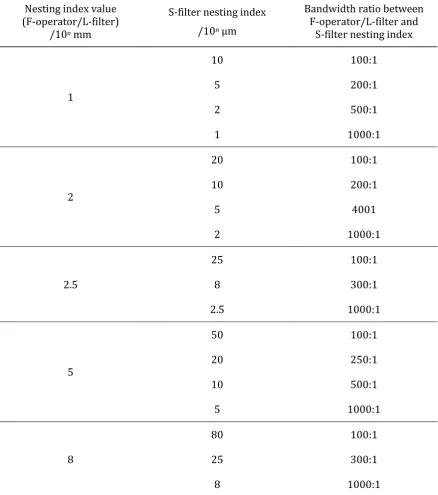
Table 1.1 Relationships between nesting index value F-operator/L-filter, S-filter nesting
index, and bandwidth ratio. n is a positive or negative integer ... 20
Table 1.2 Metrological characteristics ... 28
Table 2.1 Typical probing force values ... 42
Table 2.2 Input quantities and their associated probability density functions (PDFs). R(a, b) is a rectangular distribution and N(x, u2(x)) is a Gaussian distribution. ... 56
Table 2.3 GUM and Monte Carlo results . u(x), u(y) and u(z) are standard uncertainties ... 60
Table 2.4 Areal Instrument and NS4 step height measurements results, analysed using the method in ISO 5436-1 (2000), where σ is the sample standard deviation ... 61
Table 2.5 Uncertainty simulations results. u(x), u(y) and u(z) are standard uncertainties ... 63
Table 3.1 Types of unidimensional (profile) material measures ... 78
Table 3.2 Type of bidimensional (areal) material measures ... 79
Table 5.1 Unfiltered measurement noise of the CSI on a transparent glass flat – averaging method results ... 114
Table 5.2 Unfiltered measurement noise of the CSI on a transparent glass flat – subtraction method results ... 115
Table 5.3 Unfiltered measurement noise of the ICM instrument on a transparent glass flat – averaging method results ... 117
Table 5.4 Unfiltered measurement noise of the ICM instrument on a transparent glass flat – subtraction method results ... 117
Table 5.5 Unfiltered measured flatness of the CSI ... 120
Table 5.6 Unfiltered measured flatness of the ICM ... 121
Table 5.7 S-filter is based on the maximum sampling spacing not on the resolution of the in-strument ... 123
Table 5.8 Combined standard measurement uncertainty (uNF) contribution of the meas-urement noise and flatness deviation ... 123
Table 5.9 Combined effect of the measurement noise and flatness deviation ... 126
Table 6.1 CSI z scale calibration results ... 133
Table 6.2 ICM z scale calibration results ... 134
Table 6.3 ICM z scale calibration results - flat corrected ... 135
Table 6.4 Stylus instrument z scale calibration results ... 136
Table 6.5 Summary of the standard measurement uncertainties associated with the calibration of the z scale ... 148
Table 6.6 Summary of the standard measurement uncertainties associated with the calibration of the lateral scales when 30 µm cross-grating was used... 148
Table 6.7 Summary of the standard measurement uncertainties associated with the calibration of the lateral scales when 100 µm cross-grating was used ... 149
Table 7.1 Summary of the ICM resolution tests results with a 200 nm type ASP material measure ... 168
Table 8.1 uNF calculation ... 174 Table 8.2 Uncertainty budget associated with the measurement of a 350 nm step height standard ... 175 Table 8.3 Measurements of type ADT standard ... 179 Table 8.4 Uncertainty budget associated with the measurement of type ADT material
Figure 1.1 Geometric components of a surface profile: (a) roughness, (b) waviness, and (c)
form (Jiang et al. 2007) ... 16
Figure 1.2 Transmission characteristics of roughness and waviness profiles (ISO 4287: 1997) ... 16
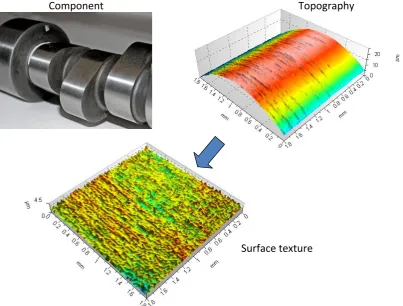
Figure 1.3 Example of surface texture measurement on a camshaft using an areal topography measuring instrument ... 19
Figure 1.4 Relationships between the S-filter, L-filter, F-operator and S-F and S-L surfaces (ISO 25178:2 2012)... 21
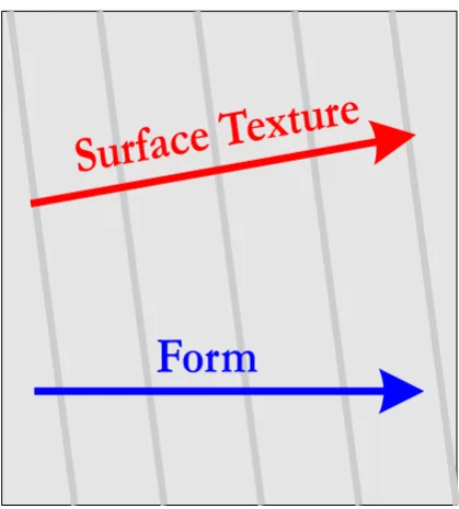
Figure 1.5 Two different coordinate systems for form and roughness ... 22
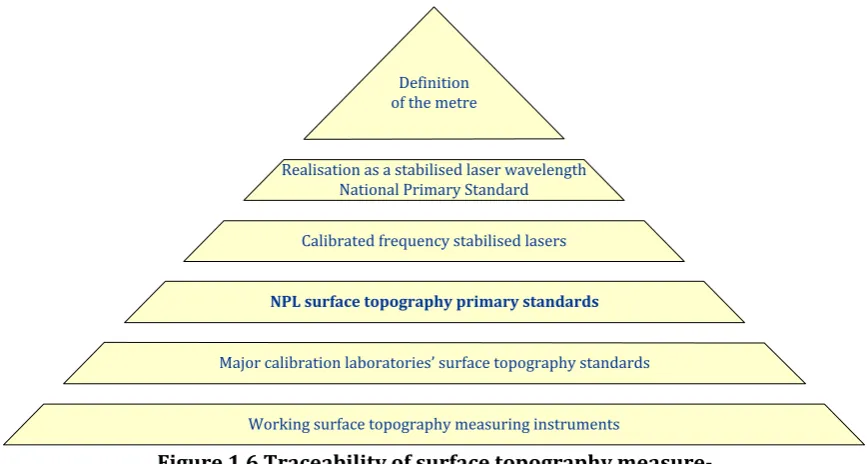
Figure 1.6 Traceability of surface topography measurements ... 23
Figure 1.7 Traceability route for areal surface texture measuring instruments ... 26
Figure 2.1 The NPL Areal Instrument ... 31
Figure 2.2 CAD model of the NPL Areal Instrument ... 32
Figure 2.3 The Zerodur mirror block ... 33
Figure 2.4 Cross-sectional representation of the probing system and its mounting ... 34
Figure 2.5 Schematic of the setup of the interferometers and sample the mount ... 35
Figure 2.6 A typical Aerotech air bearing translation stage model ABL9000 ... 36
Figure 2.7 Cross-sectional representation of the probing system, where: a) conventional di-amond stylus, b) Zerodur rod, c) mirror, d) air bearing piston, e) end of the air bearing pis-ton (part of the anti-twisting device), f) spacer, g) toroidal permanent magnet, h) aspheric lens, i) air bearing, j) anti-twisting device, k) coaxial coils, and l) heat exchanger ... 38
Figure 2.8 The probe, showing a conventional diamond stylus and Zerodur rod ... 38
Figure 2.9 Graphs showing the theoretical field strength (left) and field gradient (right) rela-tive to the distance between a permanent magnet and the physical centre of a Maxwellpair at optimum separation (Bayliss et al. 2006)... 39
Figure 2.10 Cooling coil ... 40
Figure 2.11 Modified mass balance used to test the probing force ... 41
Figure 2.12 Schema of the integrated displacement/angle interferometer ZMI2000 series (Zygo 1993) ... 42
Figure 2.13 Interferometers layout (taken and modified from Forbes and Leach (2008)) .... 43
Figure 2.14 Schematic of the x and y interferometer design (Zygo 1993) ... 44
Figure 2.15 Errors caused by metrology frame thermo-mechanics ... 45
Figure 2.16 Schematic of the z axis differential plane mirror interferometer ... 48
Figure 2.17 z axis interferometer noise test using a plane mirror ... 49
Figure 2.18 Static noise tests ... 50
Figure 2.19 Schema of a top plan view of the NPL Areal Instrument: px is the x interferome-ter position vector, wxl is the distance between the ininterferome-terferomeinterferome-ter and mirror surface, x0,l is the mirror block position vector, x(u) is a position vector that describes a point on the mir-ror, yr,l is the target position vector and yr is the target position vector in the stage refer-ence frame ... 53
Figure 2.21 Areal image of type ACG material measures 200 µm pitch and 1 µm depth ... 62
Figure 3.1 Type A1 material measure standard, from ISO 5436 1: 2000 ... 73
Figure 3.2 Type A2 material measure, from ISO 5436 1: 2000 ... 73
Figure 3.3 Type B2 and type C2 material measure, from ISO 5436 1: 2000 ... 74
Figure 3.4 Type B2 and type C1 material measure, from ISO 5436 1: 2000 ... 74
Figure 3.5 Type B2 and type C4 material measure, from ISO 5436 1: 2000 ... 74
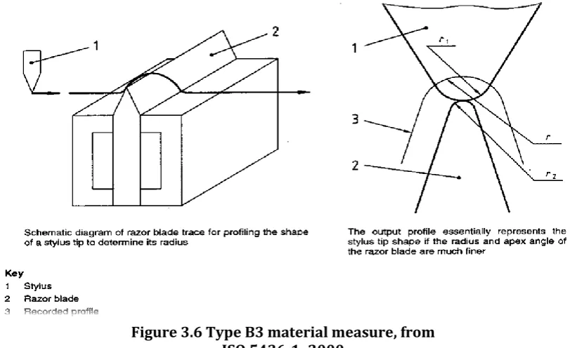
Figure 3.6 Type B3 material measure, from ISO 5436 1: 2000 ... 75
Figure 3.7 Two forms of type C3 material measures standards, from ISO 5436 1: 2000 ... 75
Figure 3.8 Type D1 material measure, from ISO 5436 1: 2000 ... 76
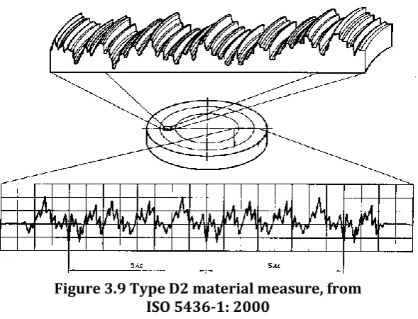
Figure 3.9 Type D2 material measure, from ISO 5436 1: 2000 ... 76
Figure 3.10 Type E2 material measure, from ISO 5436 1: 2000 ... 77
Figure 3.11 Type PAS material measure ... 80
Figure 3.12 Type AGP material measure ... 80
Figure 3.13 Type AGC material measure ... 80
Figure 3.14 Type APS material measure ... 81
Figure 3.15 Type PRI material measure ... 81
Figure 3.16 Type ACG (CG1) material measure ... 82
Figure 3.17 Type ACG (CG2) material measure ... 82
Figure 3.18 Type ADT material measure ... 83
Figure 3.19 NPL ACG type of material measure: measured (left) and design (right) ... 85
Figure 3.20 NPL resolution artefact ... 85
Figure 3.21 NPL ADT artefact ... 86
Figure 3.22 Final material measures produced in nickel: left - type ACG, right – type ADT ... 86
Figure 4.1 Roughness measuring instruments (LFM low force microscopy, MFM magnetic force microscopy, SNOM scanning near-field optical microscope) ... 89
Figure 4.2 Typical constraints in additional AW space (adapted from Stedman 1987a)... 90
Figure 4.3 Example of a measurement loop of a stylus instrument taken from ISO 3274 (1997) ... 92
Figure 4.4 Typical stylus as in ISO 25178-601, where: 1 is stylus, 2 is pivot, L is length of the arm, H is height of the stylus, rtip is radius of ... 95
Figure 4.5 Example of uniform width scar produced by a contact stylus (Griffiths 2001) ... 97
Figure 4.6 Example of uniform shock marks produced by a contact stylus on a brass sample (Mainsah et al. 2001) ... 97
Figure 4.7 Diffraction pattern of an ideal small circular aperture – airy disk (adapted from Astro Fundamentals: Light and its detection tutorial – Liverpool John Moore University). 100 Figure 4.8 Resolution limits: left Rayleigh, middle Abbe, right Sparrow (adapted from Super-resolution microscopy tutorial - the University of Utah) ... 101
modulation envelope ... 104 Figure 4.11 Imaging confocal microscope set-up ... 107 Figure 4.12 ICM axial response ... 107 Figure 5.1 Example of the result of a static noise test for a stylus instrument equivalent to a profile measurement along the fast axis of the instrument at a speed of 0.1 mm s-1, 1 µm sampling spacing and 1.4 mm sampling length... 111 Figure 5.2 Example of the result of a static noise test for a stylus instrument equivalent to a profile measurement along the fast axis of the instrument at a speed of 0.5 mm s-1, 1 µm sampling spacing and 1.4 mm sampling length... 112 Figure 5.3 Profile along the y axis of the stylus instrument resulting from averaging the topography in the x direction - first measurement noise test ... 115 Figure 5.4 Profile along the y axis of the stylus instrument resulting from averaging the topography in the x direction - second measurement noise test ... 116 Figure 5.5 Flow chart of threshold method ... 119 Figure 5.6 Flatness of a CSI that used the 20× magnification objective lens (left) and 50× magnification objective lens (right) to measure a transparent glass flat - result after ten averaged measurements ... 120 Figure 5.7 Flatness of a ICM that used the 20× magnification objective lens (left) and 50× magnification objective lens (right) to measure a transparent glass flat - result after ten averaged measurements ... 122 Figure 6.1 Example of an instrument response curve, where: 1 measured quantities, 2 input quantities, 3 ideal response curve, 4 response curve, 5 linear curve whose slope is the
Figure 6.14 Calibration of the y axis of the CSI equipped with 50× magnification lenses – error plot ... 142 Figure 6.15 Calibration of the axes of the ICM equipped with 20× magnification lenses – error plot ... 143 Figure 6.16 Calibration of the axes of the ICM equipped with 50× magnification lenses – error plot ... 143 Figure 6.17 Calibration of the x axis of the ICM equipped with 20× magnification lenses – residual errors after correcting the results using the 0. 1.001 90amplification factor ... 144 Figure 6.18 Calibration of the x axis of the ICM equipped with 50× magnification lenses – residual errors after correcting the results using the 1.001 90 amplification factor ... 144 Figure 6.19 Calibration of the y axis of the ICM equipped with 20× magnification lenses – residual errors after correcting the results using the 0.993 57 amplification factor ... 144 Figure 6.20 Calibration of the y axis of the ICM equipped with 50× magnification lenses – residual errors after correcting the results using the 0.993 57 amplification factor ... 145 Figure 6.21 Calibration of the x axis of the stylus instrument – errors plot ... 145 Figure 6.22 Calibration of the y axis of the stylus instrument – residual errors after
correcting the results using the 1.126 09 amplification factor ... 146 Figure 7.1 Example of circular profile extraction on a type ASG material measure. Batwing like effect present on the extracted profile is produced during manufacturing process ... 155 Figure 7.2 Example of linear profile extraction: left - profile extracted through the middle of two diametrically opposed raised petals; right - profile extracted through the middle of two diametrically opposed lowered petals ... 156 Figure 7.3 Height difference between the raised petals and lowered ones (optical response profile) ... 157 Figure 7.4 Normalised IRP ... 157 Figure 7.5 Example of measurement of the resolution at 50 % cut-off ... 158 Figure 7.6 CSI measurement of the type ASG material measure: left - 20× magnification lens results; right - 50× magnification lens results... 159 Figure 7.7 Measurement of the resolution at 50 % cut-off of the CSI width 20× magnification lens ... 159 Figure 7.8 Measurement of the resolution at 50 % cut-off of the CSI width 50× magnification lens ... 160 Figure 7.9 CSI measurement of a mercury droplet using 50× magnification lens ... 160 Figure 7.10 Profile extracted across the top of the mercury droplet ... 161 Figure 7.11 CSI measurement of the type ASG material measure using a 50× magnification lens with adjustable reference mirror: left – topography results; right – measurement of the resolution... 162 Figure 7.12 ICM measurement of the type ASG standard: left - 20× magnification lens
magnification lens ... 165
Figure 7.17 Measurement of the resolution at 50 % cut-off of the ICM width 50× magnification lens ... 165
Figure 7.18 ICM 20× magnification lens measurement results of the 200 nm type ASG material measure: left - 4× optical zoom; right – detail of the apex ... 166
Figure 7.19 ICM 50× magnification lens measurement results of the 200 nm type ASG material measure: left - 4× optical zoom; right – detail of the apex ... 166
Figure 7.20 ICM 50× magnification lens measurement results of the 30 nm type ASG material measure in peak mode ... 167
Figure 8.1 Measurement result of a 350 nm step height standard artefact measured using: left – stylus instrument; centre – CCI in using the 20× magnification lens configuration; and right – ICM in using the 20× magnification lens configuration ... 172
Figure 8.2 Extraction of mean profile along the x axis of stylus instrument (right) and zoom operation of the mean profile (left) ... 173
Figure 8.3 Example of step height analysis in profile mode ... 174
Figure 8.4 Measurement of a type ADT material measure using the stylus instrument ... 176
Figure 8.5 Measurement result of the central area of the ADT type standard artefact: left – stylus instrument; centre – CCI in using the 20× magnification lens configuration; and right – ICM in using the 20× magnification lens configuration ... 177
Figure 8.6 Sq measurement error plot. Error bars are the combined standard uncertainty of the instruments and of the NPL Areal Instrument ... 180
Figure A.1 x axis – pitch ... 199
Figure A.2 x axis – yaw ... 200
Figure A.3 x axis – roll ... 201
Figure A.4 y axis – pitch ... 202
Figure A.5 y axis – yaw ... 203
1
Introduction
Over the past three decades there has been an increased need to relate surface texture to surface function, which allows the manufacturer to predict how a surface interacts with its
surroundings. With such knowledge, optical, tribological, biological, fluidic and many other
properties can be altered (Evans and Bryan 1999, Bruzzone et al. 2008). To control the
manufacture of such products, traditional single line profile measurements are inadequate and an areal characterisation of surface texture is essential (Jiang et al. 2007b). A single line
profile measurement gives rise to enough information to control production, but is often
limited to looking for process change. Areal measurements offer more statistical significance and a better visual representation of the overall structure of the surface, thus providing a
more realistic representation of the whole surface (Blunt and Jiang 2003).
1.1
Historical overview
Broadly speaking, the development of surface texture characterisation followed two
strands: development of instrumentation (see chapter 4) and development of analysis tools,
both of which evolved at the same time. The first analysis tool was the Abbot-Firestone
curve (Abbott and Firestone 1933) and soon after that several researchers made the field of surface texture the formal discipline that it is today (Jiang et al. 2007a and references
there-in, Schlesinger 1942, Reason et al. 1944, Perthen 1949, Page 1948, Schorsch 1958). Three main surface components were identified: form, waviness and roughness (see figure 1.1). It
was found that the most difficult task was to separate waviness from roughness. To solve
the latter issue, two methods were proposed: one designed around a mean line system, or
M-system (Reason 1961), and one based on an envelope system, or E-system (von Weingra-ber 1956). Neither of the two systems was practical until the electrical filtering theory
(Whitehouse and Reason 1963) and, subsequently, the theory behind phase correct filters
Figure 1.1 Geometric components of a surface profile: (a) roughness, (b) waviness, and (c) form (Jiang et al. 2007)
Today, the profile standard filters are designed with an arbitrary spatial frequency cut-off which gives 50 % amplitude transmission (see figure 1.2 where λs – is the filter cut-off
which defines the intersection between the roughness and the even shorter wave
compo-nents present in the surface, λc – defines the intersection between the roughness and wavi-ness and λf – between waviness and even longer wave components) making the roughness
and waviness cut-off symmetrical and complementary (Jiang et al. 2007a).
Figure 1.2 Transmission characteristics of roughness and waviness profiles (ISO 4287: 1997)
com-puters also allowed surface visualisation to be at the fingertip of the operator. Advances made in digital filtration (in addition to increased z range and calibration procedures for
stylus instruments) meant that the same instrument could measure profile, waviness and
form. Surface texture measuring instrumentation took full advantage of the analogue to
digi-tal transformation and became more versatile.
As in the profile case, the development of areal surface texture characterisation followed
closely the advances made in areal instrumentation, which is presented in more detail in
chapter 4. Initial research (see for example Nayak (1971) and Sayles and Thomas (1977), Whitehouse and Philips (1982) and Whitehouse (1994)) highlighted the problems linked to
specification and characterisation of areal features, and the effect of the measurement
con-ditions on areal parameters (Jiang et al. 2007b). A coherent framework that allowed the
es-tablishment of areal surface texture characterisation was supported by the European Com-munity in the 1990s, which funded two major projects. The first project enabled an
integrat-ed method for the measurement and characterisation of engineerintegrat-ed surfaces (Stout et al.
1993), developing the first coherent set of areal parameters also known as ‘Birmingham 14’
(Dong et al. 1994a, b). The second project, called ‘SurfStand’ (Blunt and Jiang 2003), was
aimed towards the standardisation framework for three dimensional (3D) or ‘areal’ surface
roughness, leading to the set-up of a working group (WG16) in ISO/TC 213 in 2002. Current standardisation effort in the ISO/TC 213-WG16 in the field of areal surface texture
meas-urement includes the development of a suite of documents, under the generic title of ISO
25178, which includes definitions of terms and parameters, file formats, nominal character-istics of, and calibration methods for, areal surface topography measuring instruments.
1.2
Areal measurement
There is a wide variety of areal measurement methods dedicated to surface texture
meth-ods is the main subject of this thesis. The difference between the two classes is that the area integrating methods produce a numerical result that depends on the area-integrating
prop-erties of the surface, while the areal topography methods produce a 3D map of the surface
that can be represented mathematically as a height function z(x, y) (Leach 2011). Areal
to-pography measuring instruments are effectively co-ordinate measuring machines (CMMs) and their performance depends on a complex interaction between a number of influence
factors, such as the squareness of pairs of axes, alignment and imperfect motion (Cox et al.
1999). Whilst the effects of these interactions are usually compensated through calibration, the assessment of measurement uncertainty remains an issue.
In reality the areal topography methods are a 2½D type of investigation, not 3D, and, as a
result, undercuts and steep side walls are not measured, although some instruments can
provide more information than others depending on the design of the measuring probe. The areal map contains information about surface texture but, at the same time, it carries
infor-mation about the form of the component that is measured. For example, in figure 1.3 a cam-shaft (see figure 1.3 top left) is measured using an areal topography method. The
measure-ment result contains both form and surface texture (see figure 1.3 top right), from which a
cylinder is removed to obtain just the surface texture (see figure 1.3 bottom). Quantitative
estimation of surface texture is given by the surface texture parameters (ISO 25178-2 2012), which are calculated after filtering the surface texture data appropriately (ISO 25178-3
2012).
Surface texture parameters are affected by the size of the primary extracted surface and the sampling distance (ISO 25178-2 2012), i.e. the spatial measurement bandwidth. Setting the
measurement bandwidth is application-dependent and often requires a priori knowledge
about the surface to be measured. There are situations in which the surface to be measured
Figure 1.3 Example of surface texture measurement on a camshaft using an areal topography measuring
instru-ment
However, there are applications in which the surface, or its functionality, is not known well.
In this situation the measurement bandwidth is selected according to a priori theoretical knowledge about the nature of the surface, from prior experimental work, or a combination
of both. Unless specified, the spatial measurement bandwidth can be established in
accord-ance to ISO 25178-3 (2012), which recommends some basic rules on how to set the size of the primary surface and the sampling distance. These options are mainly based on the
choice of S-filters (surface filters which remove small scale lateral components) and L-filters
(surface filters which remove large scale lateral components)/F-operators (operators which removes form), each having a range of set values, called nesting indexes, that are
pre-sented in table 1.1 (see Leach 2013, Muralikrishnan and Raja 2010 for descriptions of areal
filtering).
Component Topography
Table 1.1 Relationships between nesting index value F-operator/L-filter, S-filter nest-ing index, and bandwidth ratio. n is a positive or negative integer
Nesting index value (F-operator/L-filter)
/10n mm
S-filter nesting index /10n µm
Bandwidth ratio between F-operator/L-filter and
S-filter nesting index
1
10 100:1
5 200:1
2 500:1
1 1000:1
2
20 100:1
10 200:1
5 4001
2 1000:1
2.5
25 100:1
8 300:1
2.5 1000:1
5
50 100:1
20 250:1
10 500:1
5 1000:1
8
80 100:1
25 300:1
8 1000:1
The S-filter nesting index determines, or is determined, by the maximum sampling distance
and the L-filter or the F-operator determines the size of primary surface (figure 1.4 presents the spatial relationship between the areal filters). The sampling distance should be chosen
after the S-filter nesting index is set; however, that is not always possible because there are
ex-tension of the cut-off wavelength from profile analysis that allows the use of the Gaussian filter and other types of filters, such as a morphological filter.
Figure 1.4 Relationships between the S-filter, L-filter, F-operator and S-F and S-L surfaces (ISO 25178:2 2012)
The S-L and S-F surfaces conceptually separate areal from profile characterisation. Unlike
the profile concept (ISO 4287 1997), where the surface features, in terms of lateral scale, are
separated in roughness, waviness and form having different coordinate systems (see figure 1.5) based on either lay direction (roughness) or parallel with the datum of the surface
(form), areal characterisation can be integrated in a uniform coordinate system in which
roughness and form are two scale components of the same surface (Jiang 2007b, ISO 25178-3 2012).
Also areal characterisation does not require a separate term for waviness but the
corre-spondence still exists (Jiang 2007b):
- Primary profile – SF-surface (λs equivalent to S-filter and nominal form removed by
F-operator);
- Waviness profile - SF-surface (λc equivalent to S-filter and nominal form removed by F-operator).
Figure 1.5 Two different coordinate systems for form and roughness
1.3
Traceability
The potential value of areal surface topography measuring instruments will only be fully
realised if the instruments provide traceable measurement results, a condition currently
only met in a few limited cases. By definition, traceability is the property of a measurement result whereby the result can be related to a reference through a documented unbroken chain
of calibrations, each contributing to the measurement uncertainty (BIPM 2008c).
Areal surface topography measuring instruments require traceability to the standard of the
metre that by definition is the length of the path travelled by light in vacuum during a time interval of 1/299 792 458 of a second, and is practically realised by an iodine-stabilised laser
(Petley 1983, Felder 2005).
For example, in the case of profile traceability, the unbroken chain of calibrations includes calibration of physical measurement standards (see chapter 3) using primary surface
topog-raphy measuring instruments that are equipped with laser interferometers of which the
Form
source is calibrated against an iodine-stabilised laser (Leach 2000); or interferometry (Teague 1978) and a contact stylus instrument; or an interference microscope (Brand 1995,
Wilkening and Koenders 2005) and a contact stylus instrument. Figure 1.6 presents an
[image:24.595.90.524.210.442.2]ex-ample of a possible traceability structure for surface topography measurement.
Figure 1.6 Traceability of surface topography measure-ments
The term calibration is often misused, which has led to confusion in understanding the
meaning of the calibration process. The frequent misuse of the term calibration is when it is
used instead of adjustment:
VIM 2.39 Note 1 – “Calibration should not be confused with adjustment of a measuring
sys-tem, often mistakenly called “self-calibration”, nor with verification of calibration.”
The adjustment process physically changes some parameters of a metrological tool (it can
be a mechanical adjustment or it could be the result of changing the value of a software con-stant) to provide an indication that is closer to a known value. The adjustment process does
not provide information about the measurement uncertainty. Similar results could be
ob-tained by correcting the measurement result using the results from a calibration certificate.
Definition of the metre
NPL surface topography primary standards
Major calibration laboratories’ surface topography standards
Working surface topography measuring instruments Calibrated frequency stabilised lasers Realisation as a stabilised laser wavelength
A meaningful measurement result can be presented without adjustment, but it has to have an associated uncertainty.
The definition of calibration, which is “operation that, under specified conditions, in a first
step, establishes a relation between the quantity values with measurement uncertainties
provided by measurement standards and corresponding indications with associated meas-urement uncertainties and, in a second step, uses this information to establish a relation for
obtaining a measurement result from an indication”, is a two stage process (BIPM 2008c
(2012)). The first stage consists of instrument calibration and the second stage involves finding the relationship between the instrument calibration results and the measurement
results. The aim of the calibration process is to have a measurement result with an
associat-ed measurement uncertainty.
1.4
Areal traceability
The work in this thesis will contribute to the provision of a traceable infrastructure to allow
modern manufacturing industry to be able to benefit from the ability to control surfaces in three dimensions.
The main theme of the project is the practical realisation of measurement traceability
through the development of an areal primary instrument, and through surface
characterisa-tion using this instrument. This work will contribute to a more complete understanding of areal surface texture.
The project delivers methodologies for using the primary instrument to calibrate areal
ma-terial measurement standards used as standard transfer artefacts. Moreover, the project es-tablishes the process of transferring this traceability to industrial users of stylus and optical
instruments according to the guidelines of the relevant ISO documents. The output of the
project will improve the understanding of surface characterisation that is required by
Currently, areal traceability is partially inferred from the measurement of standard material measures that are generally calibrated by profile measuring instruments. Whilst profile
traceability may be adequate in some circumstances, a complete traceability route for areal
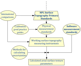
surface texture measurements requires the following elements:
Material measures for calibrating areal surface texture measuring instruments.
A primary areal surface texture measuring instrument that can measure a surface
(within a pre-determined spatial bandwidth) with traceability of its axes to the
defi-nition of the metre.
Software measurement standards for calculating areal surface texture parameters.
Methods for calculating uncertainties associated with areal surface texture measur-ing instruments and surface texture parameters.
International comparisons of areal surface texture measurements.
Good practice guides for calibrating areal surface texture measuring instruments.
Note that not long after the development of profile reference software (Bui et al. 2004, Jung
et al. 2004, Blunt et al. 2008), areal reference software was made available for testing the
calculation algorithms of the areal surface texture parameters used in commercial applica-tions (Harris et al. 2012a). Bui and Vorburger (2007) also developed independent software
for the calculation of areal surface texture parameters. The results of a comparison with a
few commercially available software packages were encouraging, as the majority of the software packages seem to agree, at least on amplitude parameters (Harris et al. 2012b).
The elements required for a complete traceability route for areal surface texture
Figure 1.7 Traceability route for areal surface texture measuring instruments
1.5
Aims of the thesis
To address the first requirement in the above list, the National Physical Laboratory (NPL)
has developed a primary areal surface texture measuring instrument. The NPL Areal In-strument is a contact stylus inIn-strument that measures the motion of a stylus tip using laser
interferometers. The interferometers are mounted on three mutually orthogonal axes
moni-toring the position of the stylus tip relative to the sample surface, providing areal measure-ments traceable to the definition of the metre.
i The first aim of this thesis is to demonstrate that the NPL Areal Instrument has the
attributes of a traceable surface texture measuring instrument, which requires the devel-opment of a model of the measurement system that faithfully represents the behaviour of
instrument.
Although the design and build of the NPL Areal Instrument were not part of this thesis, the
work on the instrument characterisation and on the measurement model led to adjustments of the design of the instrument. At the start of the project, the design of the z metrology of
NPL Surface Topography Primary
Standards
Working surface topography measuring instruemnts
Physical measurement
standards
Software measurement
standards
Calibration good practice
guides
Calculated areal surface texture parameters
Methods for calculating uncertainties International
the instrument employed an interferometer mounted in an arrangement that required de-flections of the measurement and reference beams. Due to the design of the probe (see
sec-tion 2.2) the deflecsec-tion of the beams did not allow optimal strength of the optical
interfero-metric signal. The mounting of the z interferometer had to be changed from the initial
hori-zontal position to a vertical position as shown in figure 2.2. As a result, with the NPL Areal Instrument adequate measurement results were obtained. A detailed description of the
in-strument in the final design and its uncertainty model are presented in chapter 2.
ii The second aim of the thesis was to establish the process of transferring areal trace-ability to industrial users of stylus and optical instruments according to the guidelines of the
relevant ISO documents. Basic instrument traceability is achieved by calibrating the axes of
operation of the instrument or the instrument scales. According to ISO 25178 part 601
(2010), the instrument scales of an areal topography measuring instrument should be aligned to the axes of a right handed Cartesian co-ordinate system (note that part 601 is for
stylus instruments, but the co-ordinate system will be the same for optical instruments). Practically the scales are realised by various components that are part of the metrological
loop of the instrument such that the areal map of a surface is made up of a set of points
measured along the three orthogonal axes.
Some of the instrument components provide a reference surface with respect to which the instrument measures surface topography and other components provide the vertical axis of
the instrument. So the quality and the mutual position of these components influence the
quality of areal topography measurements. Areal measurements are also affected by other factors (quantities) such as ambient temperature, mechanical and electrical noise, the
quali-ty and quali-type of the components of the instrument, the mathematical algorithms that are used
to process the height information and so on. All these factors are known as influence factors
(ISO/FDIS 25178- 603 2012). Hence, to estimate the effect of the influence factors on the measurement uncertainty, a meaningful measurement model that links the influence factors
At the outset of the project it was identified that the traceability to the industrial users had to be a simple process organised as a sequence of easy to follow, and a limited number, of
steps. The latter requirement was set in contrast to the development of ISO standards,
which for each type of instrument list a long number of influence parameters. It is very
diffi-cult, and at the same time unnecessary, to construct a mathematical model that isolates the effect of each influence factor. The influence factors approach serves well instrument
devel-opers that are required to improve their systems, and it can be used in places such as
na-tional measurement institutes and similar organisations to build complex measurement un-certainty budgets, but it is not easy to implement on the shop floor. Hence, a major task that
had to be undertaken was to convince relevant ISO committee that the benefits of the
influ-ence factor approach is only good for in depth understanding of the measuring
instrumenta-tion; however when constructing an uncertainty budget there is an easier alternative that can be used in practice.
Instead of a measurement model based on the influence factors, a simple input–output measurement model that is based on a limited number of measurable input quantities can
be used. The input quantities are called metrological characteristics and they have been
in-troduced to the ISO TC 213 WG 16. As a result, metrological characteristics are now included
in ISO/CD 25178-600 (2012) and are listed in table 1.2.
Table 1.2 Metrological characteristics
Metrological
characteristics Symbol Error along
Amplification coefficient αx, αy, αz x, y, z
Linearity lx, ly, lz x, y, z
Flatness deviation FLT-Z z
Measurement noise Nm z
Lateral period limit Dlim z
The metrological characteristics incorporate the effect of the influence factors and, more importantly, they can be measured, usually with the aid of material measures.
With the metrological characteristics in place, calibration of the instrument scales consists
of measuring the metrological characteristics of the instrument. Some of the metrological
characteristics can be affected by the size of the primary extracted surface and the sampling distance, i.e. the spatial measurement bandwidth. Along with the measurement bandwidth,
all other calibration conditions should be set in such a manner that all measurement
condi-tions are replicated (as near as possible), including the environmental condicondi-tions. Some-times, the full instrument calibration could be a very time-consuming task because it is
diffi-cult to cover all the measurement conditions in which the instrument could be used. The
situation is further complicated due to the number of software settings that are available on
commercial instruments. Fortunately, the often short measuring time of the optical instru-ments and a careful design of the experiinstru-ments can partially compensate for the number of
measurements required.
It is important to underline that the scope of this project was to find the simplest way to
achieve traceable areal surface topography measurements, which means to establish simple
procedures for testing the metrological characteristics. Hence, the method shown in this
thesis of calibrating the areal instruments is not the only route to traceability, but it was found to be relatively simple to apply in practice.
1.6
Thesis layout
As mentioned in the previous section, the design and the measurement uncertainty model of
the NPL Areal Instrument is described in chapter 2.
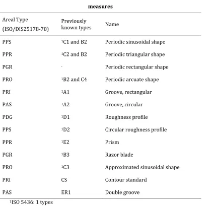
ISO/DIS 25178-70 (2012) defines several material measurement standards that can be used to calibrate areal surface texture measuring instruments. Chapter 3 reviews these material
develop-ment work aimed at producing a commercially-viable set of artefacts that can be used to cal-ibrate areal surface topography measuring instruments.
Methods for calculating uncertainties associated with areal surface texture measuring
in-struments and surface texture parameters were developed for three inin-struments, a contact
stylus and two optical instruments, which are described in detail in chapter 4. The calibra-tion on the instruments in based on the measurement of their metrological characteristics:
tests for measurement noise and residual flatness are presented in chapter 5; amplification,
linearity and squareness of the axis are treated in chapter 6; and lateral resolution is dis-cussed in chapter 7. Also, example methods for calculating areal texture parameters are
2
The
NPL
Areal
Instrument
Profile traceability is readily available at national metrology institutes NMIs either in the
form of a stylus instrument that has laser interferometers mounted on the axis of operation
Leach 2000 in the NPL case, as a combination of interferometry and a modified Taylor
Hobson Talystep 1 at NIST‐USA Teague 1978 , or a combination of interference microscopy
and Taylor Hobson Nanostep 2 instrument Garratt and Bottomley 1990 at PTB‐Germany
Brand 1995 . Although these instruments can achieve low measuring uncertainties, they
cannot be used successfully to calibrate areal surface topography measuring instruments.
Therefore, NMIs have developed primary areal surface topography measuring instruments:
NPL in the form of the NPL Areal Instrument described in this chapter ‐ see figure 2.1,
Leach 2007 ; the LUPO at PTB Thomsen‐Schmidt 2011, Thomsen‐Schmidt and Krüger‐
Sehm 2008 with a working range of 50 mm 50 mm 100 μm and an associated meas‐
urement uncertainty of 10 nm k 2 in the z direction; and a ultra high precision coordi‐
nate measuring machine at LNE Lahousse et al. 2005 with a working range of
300 mm 300 mm 50 μm and an associated measurement uncertainty of 2 nm in the z
direction.
In the next section of this chapter the overall design of the NPL Areal Instrument is de‐
scribed. Sections 2.2 and 2.3 depict the xy translation stage and the probing system, respec‐
tively, followed by a detailed description of the xy metrology in section 2.4 and of the z me‐
trology in section 2.5. The development of the measurement model is presented in section
2.6 and the uncertainty associated with the co‐ordinate measurement of the instrument is
calculated in section 2.7. The conclusions of this chapter are presented in section 2.8.
2.1
Overall
design
The NPL Areal Instrument is designed to perform traceable 3D measurement of surface tex‐
ture using a contact stylus, the position of which is monitored by laser interferometry. The
instrument monitors the relative movement of a vertically mounted stylus that is in direct
contact with the surface of a sample. A translation stage moves the sample in a nominally
horizontal plane. As the stage moves at constant speed, three linear, and two angular laser
interferometers measure the stage and stylus position in three mutually orthogonal axes. A
schema of the NPL Areal Instrument is presented in figure 2.2.
The instrument comprises a large granite base figure 2.2‐a that supports the structure of
the instrument, a coplanar air‐bearing translation stage figure 2.2‐b , a steel structural
frame figure 2.2‐c , and ancillary equipment for automation and environmental monitor‐
ing. The granite base is mounted on a passive vibration isolation table, which is in turn
mounted on four pneumatic legs. The structural frame is bolted onto the granite table above
the coplanar translation stage that itself is rigidly attached to the granite base.
The coplanar translation stage supports a sample holder and a Zerodur mirror block in the
form of a rectangular parallelepiped. The sample holder is height adjustable and is made of
Zerodur spacers having different thicknesses, allowing for coarse adjustment of the sample
height. The spacers are placed on an Invar height translation stage providing finer height
increments. The Zerodur mirror block provides the reference surface for the z axis interfer‐
ometer see figure 2.2‐e and the measurement surfaces for the x and y axis interferometers.
The mirror block thus establishes the squareness of the co‐ordinate system. The Zerodur
block is hollow with two sides removed figure 2.3 . The sample, height translation stage
and Zerodur spacers are mounted inside the Zerodur block. The outward facing sides of the
Zerodur block are polished and aluminised.
The squareness of the Zerodur block was measured using a Moore 1440 precision index and
a traceable autocollimator. The mirrors were measured to be at right angles to each other to
within 0.2 seconds of arc. The expanded uncertainty associated with the angle measure‐
ments did not exceed 0.1 seconds of arc k 2 .
The probing system figure 2.2‐d is kinematically mounted on to the steel structural frame
and can be retracted when a sample is mounted figure 2.4 .
The z axis interferometer is mounted on top of the structural frame, above the probing sys‐
tem, and the x and y axis interferometers each interferometer block is column referenced,
and contains a linear and an angular measuring system are bolted on to the underside of
the structural frame figure 2.5 . The z axis interferometer reference is obtained from the
top of the Zerodur mirror block. Since the sample is situated below the z axis reference mir‐
ror, the probe access to the sample is through a hole in the z axis reference mirror, which
limits the movement in the x and y directions to approximately 8 mm by 8 mm.
Figure2.4Cross‐sectionalrepresentationoftheprobing systemanditsmounting
The x and y axis interferometers are referenced from two further mirrors orthogonal to
each other and mounted on to the nominally stationary probing system body. Monitoring
the position of the stylus tip and translation stage using laser interferometers provides the
Figure2.5Schematicofthesetupoftheinterferometers andsamplethemount
2.2
xy
translation
stage
The coplanar air‐bearing translation stage ABL9000 was designed and manufactured for
this application by Aerotech. The stage comprises two nominally orthogonal linear position‐
ing stages. The first linear stage is aligned to travel in a horizontal plane along the system’s y
direction and the second linear stage moves in a horizontal plane along the x direction.
The working area of the xy stage is approximately 100 mm by 100 mm and the stage has
speeds ranging from 0.1 mm s‐1 up to 25 mm s‐1. The specified stage positioning resolution is
1 nm. The load is floated using an air supply pressure of approximately 410 kPa and the
stage is vacuum preloaded. The xy stage is positioned by a closed‐loop servo‐control system
Figure2.6AtypicalAerotechairbearingtranslationstage modelABL9000
Ideally, the xy metrology system should record points on a perfect rectangular grid, translat‐
ing one stage say the x axis stage from a start position to an end position in one continuous
movement a perfect grid simply makes the data analysis easier . The y axis stage is then
stepped by a fixed amount and a further x axis scan is taken, thus building up an area map in
a raster fashion. Using external interferometers for metrology, the positional repeatability is
not important, but it is preferable as it reduces the number of subsequent movements to
reach a desired position and permits for error compensation Forbes and Leach 2005 . The
straightness, xty the deviation from the true line of travel perpendicular to the direction of
travel in the horizontal plane and flatness, xtz vertical straightness were found to be bet‐
ter than 0.2 μm over the stage working range, which represents a tenth of a standard stylus
radius of 2 μm. More importantly, the stage straightness and flatness repeatability were
found to be less than 10 nm. These errors do not affect the Areal Instrument point co‐
ordinate measurement. The straightness and flatness errors generate unequal spacing be‐
tween the grid’s points that could create problems in the calculation of the surface texture
The errors in roll and pitch angles rotations around the x and y axes were found to be bet‐
ter than 0.2 seconds of arc over the stage working range 0.01 nm error for 8 mm of travel .
Although the constraints imposed on the yaw angle were not so tight, the system does not
rotate by more than 1 second of arc around its z axis 0.3 nm error for 8 mm of travel .
The measurement results of the straightness, flatness, roll, pitch and yaw errors of the air
bearing stage provided by the stage manufacturer are presented in appendix 1.
2.3
Probing
system
The instrument is required to operate over a minimum vertical range of 0.1 mm and was
designed to be capable of maintaining a constant contact force of approximately 0.1 mN –
optimal for surface texture measurements employing a 2 μm stylus tip radius – see section
4.2 throughout its vertical range. The instrument uses an air‐bearing slideway and a mag‐
netic device Bayliss et al. 2006 for balancing the probing system static load acting on the
surface, and for applying the appropriate force to maintain permanent contact between the
stylus and the surface.
The fixed part of the probing system, containing the outer cylinder of the air‐bearing and the
electromagnetic coils, is kinematically located on top of the metrology frame. This kinematic
arrangement also allows for fine adjustments of the xy interferometer reference mirrors.
The moving element of the probing system is floated by the air‐bearing that also acts as a
linear guide, and by the electromagnetic device controlling the static probing force, as
shown in figure 2.7.
The probe see figure 2.7 and figure 2.8 consists of a conventional diamond stylus
figure 2.7a attached to one end of a Zerodur rod figure 2.7b that is polished and alumin‐
ium coated at the opposite end forming a mirror ‐ figure 2.7c . The rod is coaxially mounted
inside a hollow cylinder figure 2.7d that forms the air‐bearing’s piston. One end of the pis‐
probing system is lifted up and acts as an anti‐twisting device. The probing system’s moving
piston also consists of a hollow cylinder figure 2.7f that acts as a spacer for a toroidal per‐
manent magnet figure 2.7g that is part of the electromagnetic force control, and an aspher‐
ic lens figure 2.7h , part of the z axis interferometer.
Figure2.7Cross‐sectionalrepresentationoftheprobing system,where:a)conventionaldiamondstylus,b)Zero‐
durrod,c)mirror,d)airbearingpiston,e)endoftheair bearingpiston(partoftheanti‐twistingdevice),f)spacer,
g)toroidalpermanentmagnet,h)asphericlens,i)air bearing,j)anti‐twistingdevice,k)coaxialcoils,andl)heat
exchanger
Figure2.8Theprobe,showingaconventionaldiamond stylusandZerodurrod
The air‐bearing was developed by Fluid Film Devices and has two components. The first
component is a piston‐cylinder air‐bearing figure 2.7i that operates at a pressure of ap‐
proximately 400 kPa with a gap large enough to allow the probe to move vertically while
based on a stiffness of 9 103 kg/mm . The second component is an anti‐twisting device
figure 2.7j that includes two brass components mounted on top of the air‐bearing cylinder,
acting on two lateral parallel faces of the air‐bearing piston head and preventing the probe
from turning around its vertical axis. The two brass components represent the fixed parts of
a planar air‐bearing, so that the physical contact between the probe and the fixed compo‐
nent of the anti‐twisting device is eliminated.
The electromagnetic device consists of two nominally identical coaxial coils figure 2.7k
with electrical currents passing in opposite directions. When the correct distance separates
the coils, they exhibit a region of constant field gradient near their mid point see figure 2.9 .
The optimal separation for single turn coils is equal to the coil diameter a Maxwell pair con‐
figuration .
Figure2.9Graphsshowingthetheoreticalfieldstrength (left)andfieldgradient(right)relativetothedistancebe‐
tweenapermanentmagnetandthephysicalcentreofa Maxwellpairatoptimumseparation(Baylissetal.2006)
The design uses multiple turn coils approximately 850 turns of 0.125 mm diameter enam‐
elled copper wire wound on a ceramic cylinder with an outer diameter of 12 mm, an inner
diameter of 10 mm and a length of 4 mm. The coil assembly is capable of generating suffi‐
0.2 A is applied and a 10.5 mm coil separation is used. This relatively high current produces
a significant amount of heat that can directly affect the coil assembly dimensions. The heat is
dissipated using a heat exchanger figure 2.7l and figure 2.10 made from 4 mm diameter
copper tube wrapped around the electromagnetic coil assembly. Water at ambient tempera‐
ture is circulated through the coil by a pump at a rate of forty litres per hour. The coil system
including the heat exchanger is mounted on the fixed part of the probing system via a dry
bearing, allowing for fine adjustments of the coil assembly with regards to the working posi‐
tion of the probe, or more precisely to the position of the toroidal permanent magnet.
Figure2.10Cooling coil
The static probing force was measured using a Mettler electronic balance with a resolution
of 0.1 mg, corresponding to a force of approximately 1 μN with the electromagnet coils en‐
ergised by an NPL‐designed current source Hughes and Oldfield 2003 known to provide a
very constant and precisely controllable current. The measurement of the probing force was
carried out whilst the position of the toroidal magnet inside the coil system was varied by
1 mm, with the coil current and relative position initially applied to achieve a nominal prob‐
ing force of 0.75 mN. The test showed that the probing force does not fluctuate more that
The probing force is currently monitored using a similar set‐up as described by Hughes and
Oldfield 2003 . The physical constraints of the instrument do not allow for precision mass
balance use. Instead, a modified 10 g mass balance with the resolution of 0.001 g is used
see figure 2.11 left . During the probing force measurements, the modified mass balance is
placed inside the Zerodur mirror block on top of the Invar vertical stage, allowing the stylus
tip to contact the measuring platen see figure 2.11 right . The Invar stage varies the probe
position inside the working range of the instrument whilst the nominal probe position given
by the interferometer and the corresponding probe force, measured by the mass balance,
are recorded. Typical probing forces are presented in table 2.1.
Figure2.11Modifiedmassbalanceusedtotesttheprob‐
ingforce
2.4
xy
metrology
frame
The displacement of the mirror block in x and y directions, thus the relative position of the
xy stage, is determined using a commercial laser interferometer system Zygo ZMI2000 se‐
ries utilising two linear and angular column referenced interferometers attached to the me‐
trology frame see figure 2.12 .
These two interferometers both measure the same angular yaw degree of freedom of the
Table2.1Typicalprobingforcevalues
Probe position/ mm
Probing force / N
Run 1 Run 2 Run 3
0.0 0.00 0.00 0.00
0.1 1.09 1.08 1.03
0.3 0.73 0.71 0.69
0.5 0.74 0.71 0.70
0.7 0.76 0.75 0.71
0.9 0.75 0.72 0.70
1.1 0.71 0.68 0.62
0.9 0.75 0.72 0.65
0.7 0.76 0.73 0.69
0.5 0.72 0.69 0.66
0.3 0.71 0.69 0.64
0.1 1.12 1.08 0.98
0.0 0.00 ‐0.04 ‐0.07
The helium‐neon frequency‐stabilised laser used for the x and y axis interferometers pro‐
duces a beam with two components that are collinear, orthogonally polarised and with a
heterodyne difference in frequencies of 20 MHz. The laser beam is split in two using a 50/50
beam‐splitter. The resulting laser beams are redirected to the input apertures of the x and y
axis interferometers by means of plane mirrors see figure 2.13 for interferometers layout .
The thermal effects of the interferometers’ receiver electronics are eliminated because the
light output is transmitted to the electronics via optical fibre.
Figure2.13Interferometerslayout(takenandmodified fromForbesandLeach(2008))
The resolution of the x and y axis interferometers is 0.3 nm, while the angular measurement
range is 150 seconds of arc 250 mm away from the interferometer , with a resolution of
allows the positioning of the reference mirror to be user‐defined, which leads to reduced
dead‐path errors see ω in figure 2.15 , thus the magnitude of the dead‐path effect on the
laser measurement can be decreased. Provided the measurements are always referenced
from the same initial position, the dead‐path was estimated to be 25 mm 0.6 mm k 1 .
Figure2.14Schematicofthexandyinterferometerdesign (Zygo1993)
The instrument setup minimises the Abbe offsets by ensuring that the x and y axis interfer‐
ometers are mounted in such a way that their displacement measuring arm is nominally col‐
linear with the probing system. If the interferometer beams are pointed in a direction, say
for instance in the x direction, the Abbe offsets in the y direction are estimated to be
1 mm 0.6 mm k 1 , and in the z direction, 5 mm 0.6 mm k 1 .
As the room temperature is controlled to 20 °C 0.1 °C, the metrology frame thermo‐
mechanics have only secondary effects in estimating the Abbe errors. However, the effect of
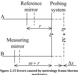
figure 2.15. The solid lines represent the system at a particular temperature t0 and the dot‐
ted lines correspond to the system at t0 t, where t is a small temperature variation of the system. The upper horizontal line, starting from point A, is the reference beam path and
the lower horizontal line, starting from point B, is the measuring beam path. The probing
system at t0, represented by the right most solid vertical line, moves naturally to a position
along the measuring direction, represented by the right most doted‐vertical line, when the
system changes its temperature by t.
Figure2.15Errorscausedbymetrologyframethermo‐
mechanics
If the base of the metrology frame is not made of similar material to the upper part, the
point of contact between the probe and the sample moves by x relative to the initial con‐ tact point. Since the interferometer will record the relative change between the measuring
mirror and the reference mirror along the measuring path, xmeasured, the error will be:
, 2.1
where is the dead‐path length at t0, r is the distance between the reference mirror and the
[image:46.595.175.444.294.551.2]per part of the metrology frame steel and for its lower part granite respectively. Consid‐
ering 25 mm, r 30 mm, 1 11.5 ‐ 5 K2 4 10‐6 KKaye and Laby 1995 and
t 0.05 °C appropriate value for a two hour scan using the NPL Areal Instrument , an er‐ ror of 4 nm is found along the measuring direction.
A further geometric error is due to the laser misalignment. The interferometers have been
aligned with deviations from the mirror surface normal smaller than thirty seconds of arc
manufacturer’s specification . This translates to a cosine error of less than 0.11 nm for a
maximum measured length of 10 mm.
The above‐mentioned errors are mainly caused by the interaction between the laser inter‐
ferometer and instrument geometry. The intrinsic properties of the laser interferometers
generate a different set of errors. The influence quantities that generate these errors can be
split into three categories, depending on which component of the laser interferometer is the
error source: laser source, interferometer characteristics and detection system Leach
1999 .
Laser source influence quantities include short and long‐term calibration of the laser fre‐