http://dx.doi.org/10.4236/ojs.2016.62027
Analysis of Variance in an Unbalanced
Two-Way Mixed Effect Interactive Model
F. C. Eze, E. U. Nwankwo
Department of Statistics, Nnamdi-Azikiwe University, Awka, Nigeria
Received 9 February 2016; accepted 23 April 2016; published 26 April 2016
Copyright © 2016 by authors and Scientific Research Publishing Inc.
This work is licensed under the Creative Commons Attribution International License (CC BY).
http://creativecommons.org/licenses/by/4.0/
Abstract
The expected mean squares for unbalanced mixed effect interactive model were derived using Brute Force Method. From the expected mean squares, there are no obvious denominators for testing for the main effects when the factors are mixed. An expression for F-test for testing for the main effects was derived which was proved to be unbiased.
Keywords
Mixed Model, Expected Mean Squares, Unbalanced Data
1. Introduction
The problem with unbalanced fixed effect interactive model is associated with the appropriate F-test for testing for the main effects when interactions are present. The paper by [1] worked on application of mixed-effects model for exposure assessment by re-analyzing three data sets from published surveys with repeated exposure measurements. The relative contributions of particular characteristics affecting exposure levels were assessed as in a multiple regression model, while controlling for the correlation between repeated measurements.
In [2], they studied a mixed-effects nonlinear regression for unbalanced repeated measures by estimating and comparing the parameters of a generalized mixed-effects nonlinear regression model. The results are applied to
in vitro data on the water transport kinetics of hemodialyzers used in the treatment of patients with chronic renal failure.
Similarly, [3] developed a method for deriving exact tests for variance components in some unbalanced mixed linear models. The derivation was based on a new kind of preliminary orthogonal transformation and a subse-quent resampling procedure. The resulting tests are based on mutually independent sums of squares which, un-der null hypothesis, are distributed as scalar multiples of chi-square variates.
of squares that are distributed independently as scalar multiple chi-square variates. These sums of squares can be used to find an exact test concerning the interaction variance components.
However, [5] considered the Two-Way ANOVA model with unequal cell frequencies without the assumption of equal error variances. They used generalized approach to finding p-values, classical F-tests for no interaction effects and equal main effects are extended under heteroscedasticity. The generalized F-test they developed in their article can be utilized in significance testing or in fixed level testing under the Neyman-Pearson theory. The problem in their work is that, the assumption of ANOVA was violated.
Analysis of variance is straightforward when an experimental design is balanced, but unequal cell sizes affect the computation of means, hypotheses tested and F-statistics [6].
Several solutions have been proposed for the analysis of unbalanced data. Solutions have focused on forcing the unbalanced data to be balanced. Suggestions include imputing cell means as additional data points into the smaller cells.
Given the model
1, 2, , 1, 2, , 1, 2, ,
ijk i j ij ijk
ij
i p
y e j q
k n
µ α β λ
=
= + + + + =
=
(1)
ijk
y is the kth observation in ijth cell;
µ
is the overall mean effects;i
α is the average effects of factor A;
j
β is the average effects of factor B;
ij
λ is the effects of the interaction between factor A and factor B;
ijk
e is a random error components and;
ij
n is the number of observations per cell.
To derive the expected mean squares for Equation (1), [7] derived the expected mean square for factor A when factor A is fixed and factor B is random as
(
)
2
2 2 2 2
. .
1 1 1
2 1 2 2 2
.
1 .. 1 . .. 1 . ..
1 .
p q q q pq
i i ij i ij ij
p p p
i j i j ij
A i i e
i i i i i
n n n n n
EMS n p
n n n β n n λ
α
α = = = σ = σ σ
= = =
= − + − + − + −
∑
∑
∑
∑
∑
∑
∑
∑
(2)According to him, in mixed models, the expected values of the sums of squares contain functions of the fixed effects that cannot be eliminated by considering linear combinations of the sums of squares. He suggested two obvious ways of overcoming the difficulties associated with unbalanced mixed effect data. The first is to ignore the fixed effects and eliminate them from the model. What remains is a random model for which the F-test can be determined. The second possibility is to assume the fixed effects as random and therefore assume the entire model as random effect models. These suggestions are in fact unsatisfactory.
2. Expected Mean Squares
2.1. Two-Way Unbalanced Random Effect Model
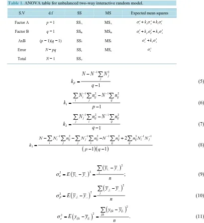
From Equation (1) above, [8] derived the expected mean squares for unbalanced two-way interactive random model.
They derive the expected mean squares for Equation (1) as shown in Table 1. Where
1 1
p q
ij i j
i j
n N N N
= =
=
∑
=∑
= (3)1 2
; 1
i i
N N N
k
p
α
−
− =
−
∑
Table 1. ANOVA table for unbalanced two-way interactive random model.
S.V d.f SS MS Expected mean squares
Factor A p − 1 SSA MSA
2 2 2
1
e kα α k λ
σ + σ + σ
Factor B q − 1 SSB MSB σe2+kβσβ2+k2σλ2
AxB (p − 1)(q − 1) SSλ MSλ σe2+k3σλ2
Error N − pq SSe MSe
2
e
σ
Total N − 1 SST
1 2
1
j j
N N N k q β − − = −
∑
(5)1 2 1 2
1
1
i ij ij
i j ij
N n N n k p − − − = −
∑ ∑
∑
(6)1 2 1 2
2
1
j ij ij
j i ij
N n N n k q − − − = −
∑ ∑
∑
(7)(
)(
)
1 2 1 2 1 2 3 1 1
3
2
1 1
i ij j ij ij ij i j
i j j i ij ij
N N n N n N n n N N
k p q − − − − − − − − + = − −
∑ ∑
∑ ∑
∑
∑
(8) and(
)
(
)
2 .. ... 2 2 .. ... ; i i a i y y E y yn
σ
−
= − =
∑
(9)(
)
(
)
2 . . ... 2 2 . . ... j j j y y E y yn
β
σ
−
= − =
∑
(10)(
)
(
)
2 . 2 2 . . ijk ij ijke ijk ij
y y E y y
n
σ
−
= − =
∑
(11)From Table 1, they found a linear combination of the mean squares with the expected mean squares and de-rived an expression for testing for
2 2 2
0: 0; 0: 0; and 0: 0.
H
σ
α = Hσ
β = Hσ
λ = (12) With the corresponding F-ratios as1 1
2
01 ,
For :H 0, Ff f MS MS α θ α α α θ σ ′
= = (13)
2 2
2
02 ,
For :H 0, Ff f MS MS β θ β α β θ σ ′
= = (14)
2
03 ,
For : 0,
e f f e MS H F MS λ λ λ
σ = = (15)
error components respectively. And
(
)
1
1
1 1 1
3
1 e ;
k MS MS MS
k
θ′ = −θ +θ λ θ = (16)
(
)
2
2
2 2 2
3
1 e ;
k MS MS MS
k
θ′ = −θ +θ λ θ = (17)
(
)
(
) (
)
(
)
1
1
2
2 2
2 2
1 1
1 e
e
MS f
MS MS
f f
θ θ
λ
λ
θ θ
′
=
− +
(18)
(
)
(
) (
)
(
)
2
2
2
2 2
2 2
2 2
.
1 e
e
MS f
MS MS
f f
θ θ
λ
λ
θ θ
′
=
− +
(19)
The sums of squares for factor A, factor B, the interaction between factor A and factor and the error terms are given by
(
)
2.. ...
A i i
i
SS =
∑
N Y −Y (20)(
)
2. . ...
B j j
j
SS =
∑
N Y −Y (21)(
)
2. .. . . ...
ij ij i j
ij
SSλ =
∑
n Y −Y −Y +Y (22)(
)
2. .
e ijk ij
ijk
SS =
∑
Y −Y (23)The expression for testing for the presence of interaction from Table 1 is
.
e
MS MS
λ (24)
2.2. Two-Way Unbalanced Mixed Effect Model
From Equation (1), if factor A is fixed and factor B is random0
i ij
i i
α = λ =
∑
∑
(25)(
2)
0,
j N β
β σ (26)
and
(
2)
0, .
ijk e
e N σ (27) Similarly, if factor A is random and factor B is fixed
0
j ij
j j
β
=λ
=∑
∑
(28)(
2)
0,
i N α
α σ (29)
(
2)
0, .
ijk e
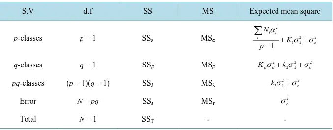
e N σ (30) Using Brute Force Method, the expected mean squares of Equation (1) when factor A is fixed and factor B is random the expected mean square are shown in ANOVA Table 2.
From Table 2, if we interested to test for the expression H0:α α1= 2==αp there are no obvious deno-minator for testing for the factor A.
However if we can obtain the expression
1
2 2 1
MSθ =Kσλ+σε (31) we would have the F-test as
1
,
f f
MS F
MS
α θ α
θ
= (32)
where fα and fθ are the numerator and denominator degrees of freedom respectively
1 2 1 2
1
where
1
i ij ij
i j ij
N n N n K
p
− −
−
= −
∑ ∑
∑
(33)
1 2
2 ij
ij
K =N−
∑
n (34)(
)(
)
1 2 1 2
3 .
1 1
ij ij i ij
ij ij i j
n N n N n K
p q
− −
− −
=
− −
∑
∑
∑ ∑
(35)
Using Welch Satterthwaite Equation fφ is the degree of freedom for the denominator and is given by
(
)
(
) (
)
(
)
1
2
2 2
2 2
1 e
e
MS f
MS MS
f f
φ φ
λ
λ
θ θ
=
− +
(36)
1
MSθ can be shown to be
(
1−θ
)
MSε +θ
MSλ (37) where1
3
.
K K
[image:5.595.69.542.100.595.2] [image:5.595.145.484.589.722.2]θ =
Table 2. ANOVA table two way unbalanced mixed interactive model when factor A is fixed
and factor B is random.
S.V d.f SS MS Expected mean square
p-classes p − 1 SSα MSα
2
2 2
1
1
i i i
N K
p λ ε
α
σ σ + + −
∑
q-classes q− 1 SSβ MSβ Kβσβ2+k2σλ2+σε2
pq-classes (p − 1)(q − 1) SSλ MSλ k3σλ2+σε2
Error N − pq SSɛ MSɛ σε2
Statement 1: Equation (37) is an unbiased estimate of Equation (31). Proof:
We take expectation on Equation (33) to have
(
)
(
)
(
)
(
)
1
2 2 2
3
2 2 2 2
3
1
1
.
E MS E MS MS K
K
θ ε λ
ε λ ε
ε ε λ ε
θ θ
θ σ θ σ σ
σ θσ θ σ θσ
= − +
= − + +
= − + +
But 1 3
K K
θ =
1
2 1 2
3 3
2 2
1 as required.
K
EMS K
K
K
θ ε λ
λ ε
σ σ
σ σ
∴ = + ⋅
= +
Similarly, if we are interested to test for factor B we have
2
0: 0
H σβ =
there would be no obvious denominator to test for the above hypothesis. However, if we can obtain the expres-sion
2
2 2
2 .
MSθ =kσλ+σε (38) We would have the F-test as
2
,
f f
MS F
MS
β θ β α
θ
= (39)
where fβ and fθ are the numerator and denominator degrees of freedom respectively.
fα is the degree of freedom for the numerator and fφ is the degree of freedom for the denominator and is given by
(
)
(
) (
)
(
)
2
2
2 2
2 2
1 e
e
MS f
MS MS
f f
φ φ
λ
λ
θ θ
=
− +
(40)
where fe and fλ are the degrees of freedom for the error components and the interactions respectively.
2
MSθ can be shown to be
(
1−θ
)
MSε +θ
MSλ (41)2
3
K K
θ =
Equation (41) is also an unbiased estimate of Equation (38).
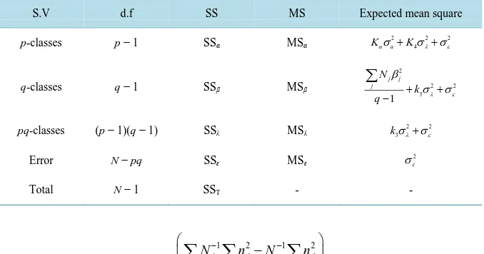
Similarly, if factor A is random, and factor B is fixed, the expected mean square are shown in the ANOVA Table 3.
Where
(
)
2 .1
i i
i
N K
p
α
α α−
=
−
∑
(42)
1 2
4
1
ij ij
N n
K p
−
= −
∑
Table 3. ANOVA table two way unbalanced mixed interactive model when factor A is ran-dom and factor B is fixed.
S.V d.f SS MS Expected mean square
p-classes p − 1 SSα MSα Kασα2+K4σλ2+σε2
q-classes q − 1 SSβ MSβ
2
2 2
5
1
j j j
N k q λ ε
β
σ σ
+ +
−
∑
pq-classes (p − 1)(q − 1) SSλ MSλ k3σλ2+σε2
Error N − pq SSɛ MSɛ σε2
Total N − 1 SST - -
1 2 1 2
5 .
1
j ij ij
j i ij
N n N n
K
q
− −
−
=
−
∑
∑
∑
(44)
When factor A is random, the hypothesis is given by
2 0: 0
H
σ
α=and there would be no obvious denominator to test for the above hypothesis. If we can obtain the expression
4
2 2 4
MSθ =kσλ+σε (45) the F-test can be shown to be
4
,
f f
MS F
MS
α θ
α α
θ
= (46)
(
)
4
4
3 1
MS MS MS
K K
θ θ ε θ λ
θ
= − +
= (47)
where fα and fθ are the numerator and denominator degrees of freedom respectively.
(
)
(
) (
)
(
)
4
2
2 2
2 2
1 e
e
MS f
MS MS
f f
φ φ
λ
λ
θ θ
=
− +
(48)
where fe and fλ are the degrees of freedom for the error components and the interactions respectively. Equation (47) is also an unbiased estimate of Equation (45).
Similarly, when factor B is fixed, the hypothesis is given by
0: 1 2 q
H β =β ==β
with no obvious denominator to test for the hypothesis. However, if we can obtain the expression
5
2 2 5
MSθ =kσλ+σε (49) the F-test can be shown to be
5
,
f f
MS F
MS
β θ β α
θ
(
)
5
5
3 1
MS MS MS
K K
θ θ θ θ λ
θ
= − +
= (51)
(
)
(
) (
)
(
)
5
2
2 2
2 2
1 e
e
MS f
MS MS
f f
φ φ
λ
λ
θ θ
=
− +
(52)
where fβ and fθ are the numerator and denominator degrees of freedom respectively. Similarly Equation (51) is also an unbiased estimate of Equation (49).
Finally, the hypothesis for testing for the presence of the interaction is given by
, f f
MS F
MS
λ ε
α λ
ε
= (53)
where fλ and fε are the numerator and denominator degrees of freedom respectively.
3. Conclusions
Equation (2) contains the functions of the fixed effect which is
2
. 1 2 .
1 ..
p
i i p
i i i i
n n
n
α
α =
=
−
∑
∑
. If we ignore the fixed ef- fects and eliminate them from the model, what remains is a random model for which the F-test can be deter-mined. The second possibility is to assume the fixed effects as random and therefore assume the entire model as random effect models. This is completely unreasonable.From Table 2 and Table 3, when one factor is fixed, we equate the functions of the fixed effect to zero and obtain an expression to determine the denominator for the F-ratio when the hypothesis is specified. Similarly, when the other factor is random, we equate the functions of the random effect to zero and obtain an expression to determine the denominator for the F-ratio when the hypothesis is specified.
To test for the interaction effect for the mixed effect model, we have
, .
f f
MS F
MS
λ ε
α λ
ε
=
This does not involve obtaining any expression and the degrees of freedom for both the numerator and deno-minator are integer valued whereas the denodeno-minator degrees of freedom for the testing for the main effects are non integer valued.
Instead of assuming both effects to be fixed or both effects to be random to enable researchers on mixed effect unbalanced interactive model analyze their data, we highly recommend our method.
This paper is limited to only an unbalanced two-way mixed effect interactive model and cannot be applied to random or fixed effect model.
4. Illustrative Example
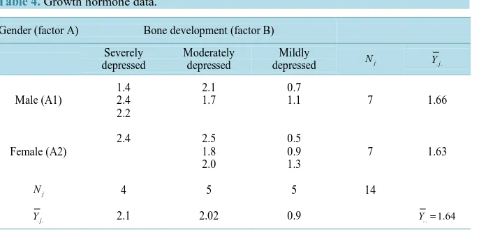
Synthetic growth hormone was administered at a clinical research center to growth hormone deficient 18 short children who had not yet reached puberty. The investigator was interested in the effects of a child’s gender (fac-tor A) and bone development (fac(fac-tor B) on the rate of growth induced by hormone administration. A child’s bone development was classified into one of the three categories: severely depressed, moderately depressed and mildly depressed. Three children were randomly selected for each gender-bone development group. The re-sponse variable (Y) of interest was the difference between the growth rate during hormone treatment and the normal growth rate prior to the treatment, expressed in centimeters per month. Four of the 18 children were una-ble to complete the study leading to unequal treatment sample sizes shown below.
Table 4. Growth hormone data.
Gender (factor A) Bone development (factor B) Severely
depressed
Moderately depressed
Mildly
depressed Nj Y. .j
Male (A1)
1.4 2.4 2.2
2.1 1.7
0.7
1.1 7 1.66
Female (A2)
2.4 2.5
1.8 2.0
0.5 0.9 1.3
7 1.63
j
N 4 5 5 14
. .j
Y 2.1 2.02 0.9 Y...=1.64
Source: Netal et al. (1996) Applied Linear Statistical Models [9].
Our hypothesis for factor A shall be
2 0: 0.
H
σ
α =Using Equations (20), (22) and (23) we have
0.0035; 1.242 and 0.1625.
A e
MS = MSλ = MS =
Similarly, using Equations (43) and (44)
4
4 5 3
3
2.57, 1.29 and 1.87; hence K 1.37.
K K K
K
θ
= = = = =
From Equations (47) and (48)
4
4
0.05 1,2
1.641 and 1.8621 0.0035
0.00213 1.641
18.51.
A
MS f
MS F
MS F
θ θ
θ
= =
∴ = = =
=
Our conclusion is that we do not reject the null hypothesis. Similarly, our hypothesis for factor B shall be
0: 1 2 3.
H β =β =β
Using Equation (21)
2.153.
MSβ =
From Equations (51) and (52)
5
5
0.05 2,2
0.91 and 2.25
2.153 2.37 0.91
19.00.
MS f
MS F
MS
F
θ θ
β
θ
= =
∴ = = =
=
Our conclusion is that we do not reject the null hypothesis. Finally, to test for the interaction we have
0.05 2,8
1.242 7.64 0.1625
4.46.
MS F
MS
F
λ
ε
= = =
=
References
[1] Peretz, C., Goren, A., Smid, T. and Kromhout, H. (2002) Application of Mixed-Effect Models for Exposure Assess-ment. Annals of Occupational Hygiene, 46, 69-77. http://dx.doi.org/10.1093/annhyg/mef009
[2] Edward, F.V. and Randy, L.C. (1992) Mixed-Effect Nonlinear Regression for Unbalanced Repeated Measures.
Biome-trics, 48, 1-17. http://dx.doi.org/10.2307/2532734
[3] Ofversten, J. (1993) Exact Tests for Variance Components in Unbalanced Mixed Linear Models. Biometrics, 49, 45- 57. http://dx.doi.org/10.2307/2532601
[4] Khuri, A.I. and Littell, R.C. (1987) Exact Tests for the Main Effects Variance Components in an Unbalanced Random Two-Way Model. Biometrics, 43, 545-560. http://dx.doi.org/10.2307/2531994
[5] Ananda, M.M.A. and Weerahandi, S. (1997) Two-Way ANOVA with Unequal Cell Frequencies and Unequal Va-riances.Statistica Sinica, 7, 631-646.
[6] Dawn, I. (1995) Analysis of Variance for Unbalanced Data. Marketing, Theory and Practice, 6, 337-343. [7] Searle, S.R. (1971) Topics in Variance Components Estimation. Biometrics, 27, 1-76.
http://dx.doi.org/10.2307/2528928
[8] Eze, F.C. and Chigbu, P.E. (2012) Unbalanced Two-Way Random Model with Integer-Value Degrees of Freedom.
Journal of Natural Sciences Research, 2, 100-107.