Optimal Power Flows with Security Constraints Using
Multi Agent based PSO Algorithms by Optimal
Placement of Multiple SVCs
K. Ravi Kumar
Associate ProfessorEEE Department Vasavi College of Engineering,
Hyderabad
S. Anand
Senior Software AnalystIntergraph Consulting Hyderabad
M. Sydulu
Phd, Professor ,EE Department National Institute of Technology,
Warangal
ABSTRACT
This paper puts forward the implementation of multiagent based PSO algorithms (TDLSMADSO & CLSMAPSO) to obtain the optimal power flows by optimally placing SVC devices. The static var compensator (SVC) is modeled using susceptance model with modifications in the Y bus of the Newton Raphson Algorithm. The constraints related to violation limits, minimization of voltage stability index, and line loss are dealt using penalty factor approach. The new multi agent based cubic lattice and two dimensional lattice structured based PSO algorithms were considered for optimizing power flows while satisfying all the constraints mentioned above. These algorithms were tested on IEEE 30 and IEEE 14 bus systems to identify the suitable location, its susceptance value and firing angle. The results obtained were quite encouraging and will be useful in electrical restructuring.
General Terms
Multi agent systems, Particle swarm optimization, Optimal power flows, security constraints, Static VAR compensator, FACTS (Flexible AC transmission systems)
Keywords
Multi agent systems, Optimization techniques, Particle swarm optimization, Optimal power flows, security constraints.
1.
INTRODUCTION
Now a days, utilities are facing rapid increase in electricity demand with slow reinforcement projects due to financial and political issues. Proper operation and planning requires consideration of various factors such as reduction of generation cost, losses, security of power system, and FACTS application etc. In this aspect, the optimal power flows has become the leading research field with potential applications for both planning and operation of power system. An operational point of a power system not only is a stable equilibrium of differential and algebraic equations (DAE), but also must satisfy all of the static constraints of the equilibrium such as upper and lower bounds of generations, voltages of all buses and line flow units of all the transmission lines. This operation point in the power system is solved by OPF. In other words, OPF is to minimize the operating costs of the power system, transmission losses or other appropriate objective functions at the specified time
corresponding to power output of generators, transformer tap positions, phase shifter angle positions, shunt capacitors / reactors values, voltage values etc. Conventionally, OPF is used to solve security and economic operation of the power system. A wide variety of optimization techniques have been applied in solving the OPF problem such as non-linear programming, Quadratic Programming, Linear Programming, Newton based methods, Sequential unconstrained minimization technique, interior point methods, Genetic Algorithm, Evolutionary Programming. Heuristic algorithms such as Genetic Algorithms (GA) and Evolutionary programming which have been reported as show promising results for further research in this direction. Recently, a new evolutionary computation technique, called Multi agent based Particle Swarm Optimization (MAPSO)2, has been proposed. Particle Swarm Optimization (PSO) is one of the evolutionary computation techniques. In PSO, search for an optimal solution is conducted using a population of particles, each of which represents a candidate solution to the optimization problem. It was developed through the simulation of flock of birds to search for food in an optimal manner through their velocity and position up gradation. The PSO technique has been widely used for the optimization of various power system problems. However, the major drawback with PSO is that, it may need several iterations and may get trapped in local optima. Therefore, several strategies have been developed to overcome the limitations of PSO, such as modified PSO, and attractive and Repulsive PSO. These all were proved to be effective and boosted the development of MAPSO.
and they can also use their own knowledge. With the search mechanism of PSO and agent-agent interactions, TDLSMAPSO and CLSMAPSO can obtain global solution with faster convergence characteristics.
Today technologies developed as a part of flexible AC Transmission system (FACTS) can be handy to corrective methods, so that the system operates smoothly and consistently without violating thermal and operational limits. FACTS devices, which permit to achieve many objectives in an electric power system [5, 8, 9, 10] can be used to reduce the power flow on the overloaded lines and to increase the utilization of the existing transmission lines. This allows to increase the transfer capability in existing transmission and distribution systems under normal conditions, obtaining the possibility to load lines much closer to their thermal limits.
Similarly, shunt FACTS devices such as SVCs will inject reactive power into the transmission system so that it improves the voltage profiles of the different buses of the power system. While placing the devices we need to identify the best location based on various factors such as voltage stability factor, reduction of total fuel cost, reduction of losses etc.
This paper is organized as follows: FACTS device modeling and Problem formulation were discussed in section 2. Two dimensional and Cubic lattice structured Multi agent based PSO approaches in section 3. Implementation of PSO, TDLSMAPSO and CLSMAPSO for optimal placement of SVCs along with OPF is discussed in section 4. The simulation results are discussed in section 5. Finally, brief conclusions are deduced in section 6 and references in section 7.
2.
PROBLEM FORMULATION
2.1. SVC Model:
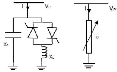
The steady state model is proposed here to incorporate the SVC in the Newton – Raphson Load flow solution [5]. This model is based on representing the controller as a variable impedance, assuming an SVC configuration with a fixed capacitor (FC) and Thyristor Controlled Reactor (TCR) as shown in Fig.1. Applying gate pulses simultaneously to all thyristors, comes into conduction. The thyristors will block approximately at zero crossing of AC current, in the absence of firing signals. The thyristors are fired symmetrically in an angle control range of 900 to 1800 with respect to the capacitor voltage.
In our work, the effect of SVC is considered by changing the bus admittance values corresponding to the bus admittance matrix in which the SVC is placed. The reactive power injected at the SVC node is given by Q = -BSVCV2.
Fig 1. SVC Configuration and its Susceptance model 2.2 Objective Function:
The OPF problem is a static constrained non-linear optimization problem, the solution of which determines the optimal settings of control variables in a power system network satisfying various constraints. Hence, the problem is to solve a set of non-linear equations describing the optimal solution of power system. It is expressed as
Min F(x,u) (1)
Subject to g(x, u)=0 h(x, u)≤0
The objective function F is fuel cost of thermal generating units of the test system. g(x,u) is a set of non-linear equality constraints to represent power flow and h(x,u) is a set of non-linear inequality constraints(i.e., bus voltage limits, line MVA limits etc..). Vector x consists of dependent variables and u consists of control variables.
In most of the non-linear optimization problems, the constraints are considered by generalizing the objective function using penalty terms. In this OPF problem, slack bus power PG1, bus voltages VL and line flows Ij are constrained by adding them as penalty terms to objective function. Hence, the problem can be generalized and written as follows.
[ ∑ ∑
∑ ( ) ∑
]
Where , the penalty factor, is given as
∑
and are defined as
{ (3)
{
[image:2.595.346.535.75.192.2]Where IC is the Installation cost of the device given by IC= C x S x1000+PF x ‖ ‖ (5)
Where C = Cost of installation of FACTS devices in US $/KVAR;
PF = Penalty Factor, value ranges from 1030 to 1035; S = Operating range of FACTS devices in MVAR; CSVC=0.0003S2-0.3051S+127.38
J = ∏
Where VS = Voltage Stability index
VS = { | |
Vb is the voltage at bus b and
3.
TWO DIMENSIONAL AND CUBIC
LATTICE STRUCTURED MULTI
AGENT BASED PSO APPROACHES
3.1 PSO
The inherent rule adhered by the members of birds and fishes in the swarm, enables them to move, synchronize, without colliding, resulting in an amazing choreography which is the basic idea of PSO technique. PSO is a similar Evolutionary computation technique in which, a population of potential solutions to the problem under consideration, is used to probe the search space. The main difference between the other Evolutionary Computation (EC) techniques and Swarm intelligence (SI) techniques is that the other EC techniques make use of genetic operators whereas SI techniques use the physical movements of the individuals in the swarm. PSO is developed through the bird flock simulation in two-dimensional space with their position, x and velocity, v.
The optimization of the objective function is done iteratively through the bird flocking. In every iteration, every agent knows its best so far, called ‘Pbest’, which shows the position and velocity information. This information is analogous to personal experience of each agent. Moreover, each agent knows the best value so far in the group, ‘best’ among all ‘Pbest’. This information is analogous to the knowledge, as to how the other neighboring agents have performed. Each agent tries to modify its position by considering current positions, current velocities, the individual intelligence (Pbest), and the group intelligence (Gbest).
To ensure the best convergence to PSO, Eberhart and Shi indicate that use of constriction factor may be necessary. The modified velocity and position of each particle can be found as follows.
(
) (5)
(6)
Where d indicates the generation, xd is the current position of the particle in dth generation, vd is the velocity of the particle in the dth generation, ω is the inertia weight, C1 and C2 are acceleration constants, and and are the constriction factors. The constriction factor is been updated by the following equations for PSO and CLSMAPSO respectively. By making use of this updating, variable constriction factor can be adapted so that the convergence can be achieved quickly.
) for PSO (7)
for (8) TDLSMAPSO and CLSMAPSO
Here, the values of and vary from iteration to iteration. The “Initial error” is the maximum deviation between the fitness values of the agents in the first iteration and “error” is the maximum deviation between the agents at iteration. In case of normal PSO the position vector is updated only by velocity vector. In case of TDLSMAPSO and CLSMAPSO, the position vector is updated by both velocity and competition and cooperation operators. Hence and cannot be equal for both inertial and dynamic terms of velocity if we have to get CLSMAPSO converged faster. The velocity of every agent must be updated in such a way that it decreases as the agent converges and increase as the agent diverges. The exponents and multipliers are selected randomly in the equations (7) and (8) as with these values the algorithm converges faster. In PSO, the particle velocity is limited by some maximum value Vmax. If V max is too high, particles may fly past good solutions. If Vmax is too small, particles may not cross local solutions. Normally Vmax is taken as 10% - 20% of dynamic range and Vmin is selected as - Vmax..
(9)
3.2. Multi Agent Systems
According to Wooldridge, an agent is a physical or virtual entity that has the following properties.
i. It lives in and acts in the environment.
ii. It senses its local environment through its interaction with the other agents.
iii. It will attempt to achieve some goals and execute certain tasks.
iv. It will respond to the environment through the self learning.
Multi agent systems are computation based systems in which several agents interact and work in coordination with one another to achieve some goals and perform certain tasks. In general, there are four things need to be defined when we are solving problems using multi agent systems.
i. Meaning and purpose of the agent. ii. Environment where all agents live.
iii. Definition of the local environment to know the local perceptivity.
3.3. TDLSMAPSO
[image:4.595.345.507.71.168.2]In TDLSMAPSO, multi agents are being arranged in a square lattice structure and is been integrated with PSO to form a new approach called as TDLSMAPSO. Each agent represents a particle to PSO and a candidate solution to OPF problem. Since all the agents live in square lattice structured environment as in Fig.1, each agent can interact with all the neighbors. Using the competition, cooperation and PSO operators, the global solution is achieved.
3.4. CLSMAPSO
In CLSMAPSO, multi agents are being arranged in a cubic lattice structure and is been integrated with PSO to form a new approach called as CLSMAPSO. Each agent represents a particle to PSO and a candidate solution to OPF problem. Since all the agents live in cubic lattice structured environment as in Fig.2, each agent can interact with all the neighbors. Using the competition, cooperation and PSO operators, the global solution is achieved.
The following are the essential before realizing the actual algorithms of TDLSMAPSO and CLSMAPSO:
3.4.1. Agent for OPF Problem
In CLSMAPSO, each agent is a particle to PSO and a candidate solution to OPF problem. Therefore, every agent λ has a fitness value to the OPF problem. The fitness value is the value of generation cost, i.e., FT .
FT(λ) =∑ (10)
3.4.2. Definition of an Environment
In TDLSMAPSO, all agents live in an environment which is of square lattice-like structure as in Fig. 2. In the environment L, each agent is placed on a lattice-point and each circle represents an agent. The size of L is Lsize ×Lsize where Lsize is an integer. In TDLSMAPSO, number of particles and L should be same.In CLSMAPSO, all agents live in an environment which is of cubic lattice-like structure as in Fig. 3. In the environment L, each agent is placed on a lattice-point and each circle represents an agent. The size of L is Lsize ×Lsize ×Lsize where Lsize is an integer. In CLSMAPSO, number of particles and L should be same.
3.4.3. Definition of the Local Environment
Since each agent can only sense its neighbours, it is very important to define the local environment. In this paper, in TDLSMAPSO, an agent λ located at (i,j) can have 8 neighbours (including 4 sides and 4 corners ) as it can be seen from the lattice and in CLSMAPSO,an agent λ located at (i,j) can have 26 neighbours (including 6 sides, 8 corners and 12 edges) as it can be seen from the lattice.
[image:4.595.336.514.211.362.2]Figure 2. Square Lattice structure of Multi agent system for PSO
Figure 3. Cubic Lattice structure of Multi agent system for PSO
3.4.4.Behavioural Rules for Agent
In TDLSMAPSO and CLSMAPSO, every agent competes and cooperates among its neighbours and makes use of evolution mechanism and knowledge of PSO and hence it diffuses all its information to whole environment. Based on the behaviours, the competition and cooperation operator were designed and are as follows.
3.5. Competition and Cooperation Operator
Suppose that competition and cooperation operator ios performed on the agent λ located at (i,j) and λi,j=( λ1 ,λ2 , ...λn) and Mini,j=( m1 ,m2 , ...mn) is the agent with minimum fitness value among its neighbours, namely Mini,jϵNeighboursi,j. If agent λi,j satisfies the following equation it is a winner otherwise it is a loser.
( ) ( ) (11) If λi,jis a winner, it can still live in the agent lattice. If λi,j is aloser, it must die and its lattice-point will be occupied by Newi,j. The new agent Newi,j =( , ) is determined by the following strategy
min,max, min,max,if ( (0,2.5 * (error/initial_error)) x( ))
if (0,2.5 * (error/initial_error)) x (
( (0,2.5 * (error/initial_error)) x (
' ( ))
k k k
k k k
k k k
rand
rand m
k
rand
k k
k k
x x
x x
m m
m m
m
)) otherwise
1, 2,...,
k n
While minimizing the total generation cost, the total generation should be equal to the total system demand plus the transmission network loss.
4.
IMPLEMENTATION
4.1. Algorithm for SVC Placement
The step by step algorithm for the proposed optimal placement of SVCs for optmal power flows is given below:
1. Read data from file
2. Formulate Ybus without FACTS devices 3. Initialize PSO algorithm with PSO parameters c,r1,c2,r2,inertia.
4. Set position and velocity limits for a position vector.
5. Call PSO algorithm that internally calls objective function for fitness value.
6. After PSO execution is completed, output the Position vector to console.
4.2. Algorithm for Objective Function Evaluation
1. Get the pgi values from the position vector for each pv bus
2. Get the position (bus number for SVC device) and Firing angle for each FACTS Device.
3. With the position and firing angles for each FACTS device, find the effective values of reactances for each FACTS device.
4. Modify the originally calculated Y bus with the reactances calculated above.
5. Find the load flow solution by calling NR algorithm.
6. From the N- R Algorithm solution, using security constraints, compute the penalties.
7. From the PGis of PV buses and from the solution of NR, Find PGi of slack bus.
8. Find the operating cost & FACTS device costs. 9. Output the fitness value as the sum of operating cost, FACTS device costs and the penalties.
In TDLSMAPSO and CLSMAPSO, mainly the operators were used to obtain the optimal solution in quick time with accuracy. Among them competition and cooperation operators along with PSO operators were used.
4.3. Algorithm of TDLSMAPSO and CLSMAPSO for OPF Problem
1. Input the parameters and specify lower and upper Limits of variables. In OPF problem, PGi, i ϵ NG except for slack bus are the variables.
2. Determine the fitness value of each agent i.e., Production cost, by Newton-Raphson power flow analysis results.
3. Sort the particles.
4. Create a lattice like environment L, and assign each agent (which is essentially a particle) on lattice point in the ascending order. Here each
except slack bus power. 5. Increment the iteration counter
6. Carryout competition and cooperation operator on each agent and modify it.
7. Apply PSO mechanism to each agent and adjust its position using velocity and position equations. 8. Determine the fitness value of each agent i.e., production cost, by Newton-Raphson power flow analysis results
9. Determine the best agent with minimum fitness value.
10. Sort the particles in ascending order. 11. Check for stopping condition (all the agents converge to a fitness value), if yes go to next step, else go to step (4).
12. Print the agent and its fitness value.
Table 1. Parameters for PSO,TDLSMAPSO , CLSMAPSO and the SVC Parameters
S.No Parameter Value
1. c1 0.6
2. c2 0.4
3. r1 0.6
4. r2 0.4
5. No. of Particles 64
6. SVC Parameters Xl=2.5 p.u and
Xc=15 p.u
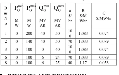
Table 2. Generator Data With Quadratic Cost Functions Considered for IEEE 30 Bus System
Bu s No min G
P
M W max GP
MW min GQ
MVA R max GQ
MVA R a $ / h r B $/M Whr C $/MW²hr1 50 200 -20 200 0 2.0 0.00375
2 20 80 -20 100 0 1.75 0.0175
5 15 50 -15 80 0 1.0 0.0625
8 10 35 -15 60 0 3.25 0.00834
11 10 30 -10 50 0 3.0 0.0250
[image:5.595.311.543.560.706.2]13 12 40 -15 60 0 3.0 0.0250
Table 3. Generator Data With Quadratic Cost Functions Considered for IEEE 14 Bus System
B us N o min G
P
M W max GP
M W min GQ
MV AR max GQ
MV AR a $/ hr B $/M Whr C $/MW²hr1 0 200 40 50 10
0 1.083 0.074
2 0 140 40 50 70 1.033 0.089
3 0 100 0 40 10
0 1.083 0.074
6 0 100 6 24 70 1.033 0.089
8 0 100 6 25 40 1.17 0.053
5.
RESULTS AND DISCUSION
The SVCs were set to be placed optimally with a goal that the power low and generation should be optimal . To verify as well as to compare the effectiveness of the algorithms the results obtained were compared with[ 5, 9]. Table summarizes the optimal power flow results with different algorithms.
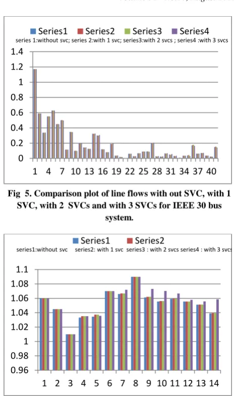
The algorithm is implemented in C programming language and executed on Intel Core 2 Duo system with 1GB RAM running on linux. The solutions for optimal location of SVCs to minimize the generation cost subject to minimize the cost of installation and so that it improves the voltage stability of the system. The IEEE14 and IEEE 30 bus systems were obtained and discussed below. The simulation studies were carried out on Pentium IV, 2.4 GHz system in LINUX environment All the three algorithms PSO, TDLSMAPSO and CLSMAPSO were applied for optimal power flows and also to identify the optimal location of SVCs. Initially the algorithms were tested with one SVC, later with two SVCs and finally tested with three SVCs. The results were listed in the tables below. Fig.4 and Fig.6 shows the Comparison plot of voltage profile without SVC, with 1SVC, with 2SVCs and 3 SVCs for IEEE 30 and IEEE 14 bus systems respectively. Fig.5 and Fig.7 shows the Comparison plot of Line Flows without SVC, with 1SVC, with 2SVCs and 3 SVCs for IEEE 30 and IEEE 14 bus systems respectively.
[image:6.595.307.539.56.448.2]From the figures (Fig .4 to Fig.7),for both the IEEE 14 and IEEE 30 bus systems, it is evident that, after the placement of SVC devices, the voltage profile has been improved. It is also observed that, the Line flows in the lines have also been improved. Due to the limitation of cost, we have limited our investigation only up to three devices.
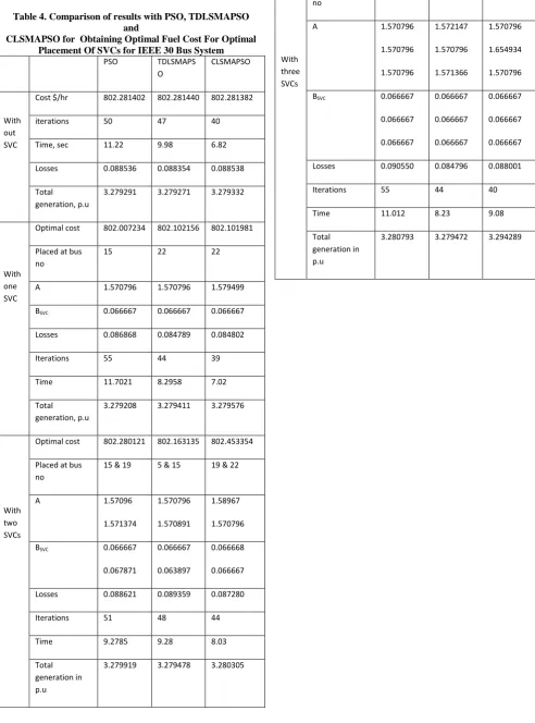
Table. 4 and Table.5 shows the Comparison of results with PSO, TDLSMAPSO and CLSMAPSO for Obtaining Optimal Fuel Cost For Optimal Placement Of SVCs for IEEE 30 and IEEE 14 bus Systems. It is quite evident from the results shown in the tables that, the line losses were reduced and the line flows were improved. With the optimal location of SVCs the optimal generation schedule was obtained.
[image:6.595.310.538.71.238.2]Fig 4. Comparison plot of voltage profile without SVC, with 1SVC, with 2SVCs and 3 SVCs for IEEE 30 bus system
Fig 5. Comparison plot of line flows with out SVC, with 1 SVC, with 2 SVCs and with 3 SVCs for IEEE 30 bus
system.
Fig 6. Comparison plot of voltage profile of IEEE14 bus system with out SVC, with 1 SVC, with 2 SVCs and with 3
[image:6.595.307.538.472.636.2]SVCs.
Fig 7. Comparison plot of line flows with out SVC, with 1 SVC, with 2 SVCs and with 3 SVCs for IEEE 14 bus system.
From the above four figures(Fig .4 to Fig.7),for both the IEEE 14 and IEEE 30 bus systems, it is evident that, after the placement of SVC devices, the voltage profile has been improved. It is also observed that, the Line flows in the lines have also been improved. Due to the limitation of cost, we have limited our investigation only up to three devices. It is also been observed that, the optimal cost has been attained with the 0.85
0.9 0.95 1 1.05 1.1 1.15
1 3 5 7 9 11 13 15 17 19 21 23 25 27 29
Series1 Series2 Series3 Series4
series1:without svc series2:with 1 svc series3 : with 2 svcs series4 : with 3 svcs
0 0.2 0.4 0.6 0.8 1 1.2 1.4
1 4 7 10 13 16 19 22 25 28 31 34 37 40
Series1 Series2 Series3 Series4
series 1:without svc; series 2:with 1 svc; series3:with 2 svcs ; series4 :with 3 svcs
0.96 0.98 1 1.02 1.04 1.06 1.08 1.1
1 2 3 4 5 6 7 8 9 10 11 12 13 14
Series1 Series2
series1:without svc series2: with 1 svc series3 : with 2 svcs series4 : with 3 svcs
0 0.2 0.4 0.6 0.8
1 3 5 7 9 11 13 15 17 19
Series1 Series2 Series3 Series4
[image:6.595.55.294.507.677.2]placement of devices along the reduction in the losses. Tables 4 and 5 indicate the iterations , time for computation optimal cost , losses and Total generation in per unit.
Table 4. Comparison of results with PSO, TDLSMAPSO and
CLSMAPSO for Obtaining Optimal Fuel Cost For Optimal Placement Of SVCs for IEEE 30 Bus System
PSO TDLSMAPS
O
CLSMAPSO
With out SVC
Cost $/hr 802.281402 802.281440 802.281382
iterations 50 47 40
Time, sec 11.22 9.98 6.82
Losses 0.088536 0.088354 0.088538
Total generation, p.u
3.279291 3.279271 3.279332
With one SVC
Optimal cost 802.007234 802.102156 802.101981
Placed at bus no
15 22 22
Α 1.570796 1.570796 1.579499
BSVC 0.066667 0.066667 0.066667
Losses 0.086868 0.084789 0.084802
Iterations 55 44 39
Time 11.7021 8.2958 7.02
Total generation, p.u
3.279208 3.279411 3.279576
With two SVCs
Optimal cost 802.280121 802.163135 802.453354
Placed at bus no
15 & 19 5 & 15 19 & 22
Α 1.57096
1.571374
1.570796
1.570891
1.58967
1.570796
BSVC 0.066667
0.067871
0.066667
0.063897
0.066668
0.066667
Losses 0.088621 0.089359 0.087280
Iterations 51 48 44
Time 9.2785 9.28 8.03
Total generation in p.u
3.279919 3.279478 3.280305
With three SVCs
Optimal cost 803.089332 802.773648 802.693581
Placed at bus no
5, 15 &30 5,7 &22 5,19 &23
Α 1.570796
1.570796
1.570796
1.572147
1.570796
1.571366
1.570796
1.654934
1.570796
BSVC 0.066667
0.066667
0.066667
0.066667
0.066667
0.066667
0.066667
0.066667
0.066667
Losses 0.090550 0.084796 0.088001
Iterations 55 44 40
Time 11.012 8.23 9.08
Total generation in p.u
Table 5. Comparison of results with PSO, TDLSMAPSO and
CLSMAPSO for Obtaining Optimal Fuel Cost For Optimal Placement Of SVCs for IEEE 14 Bus System
PSO TDLSMAPSO CLSMAPSO
With out SVC
Cost $/hr 1660.927965 1662.934461 1660.927976
Iterations 62 76 76
Time, sec 2.418 2.75 3.011
Losses 0.013694 0.0136765 0.013694
Total generatio n, p.u
0.944860 0.945234 0.944861
With one SVC
Optimal cost
1660.914608 1659.932127 1659.932574
Placed at bus no
5 5 1
α, rad 1.571261 1.570796 2.036498
BSVC 0.066667 0.066667 0.082453
Losses 0.013652 0.013552 0013285
Iterations 63 72 64
Time 2.652 3.49 2.76
Total generatio n, p.u
0.946612 0.946612 0.927129
With two SVCs
Optimal cost
1660.949970 1660.565803 1659.74709
Placed at bus no
5 & 8 5 & 7 1 & 3
α, rad 1.57096
1.57096
1.790135
1.570796
2.044786
1.573409
BSVC 0.066667
0.066667
0.0712025
0.066667
0.083285
0.066667
Losses 0.013659 0.013757 0.013078
Iterations 66 75 71
Time 2.995 3.51 3.322
Total generatio n in p.u
0.946914 0.933712 0.924284
With three SVCs
Optimal cost
1660.690554 1660.410232 1659.546271
Placed at bus no
5, 15 &30 1,5 & 11 1, 8 &14
α, rad 1.570796
1.570796
1.570796
1.880084
1.570796
1.571366
2.011458
1.570796
1.571285
BSVC 0.066667
0.066667
0.066667
0.071405
0.066667
0.066667
0.080102
0.066667
0.066667
Losses 0.013843 0.013251 0.013352
Iterations 66 73 89
Time 3.448 3.573 4.062
Total generatio n in p.u
0.946653 0.930887 0.928895
6.
CONCLUSION
Based on multi agent systems, TDLSMAPSO and CLSMAPSO have been developed for solving Optimal power Flow problem (OPF) with optimal placement of SVCs along with security constraints. To the best of our knowledge, OPF problem has been solved by several methods in the literacy but these unique TDLSMAPSO and CLSMAPSO methods integrates the square and Cubic Lattice Structured multi agents respectively for TDLSMAPSO and CLSMAPSO with PSO using variable constriction factor to find the global or near global optimum point for OPF problem along with the optimal location of SVCs. IEEE 14 and IEEE 30 bus systems have been tested s and results are compared. From the results, TDLSMAPSO and CLSMAPSO converges to global optimum with more accuracy and within less time. From the results, CLSMAPSO converges to global optimum with an accuracy of 0.0001 and within less time. It can be observed that PSO is consuming more time and iterations to converge, where as TDLSMAPSO and CLSMAPSO were consuming less time and less number of iterations to obtain near optimum solution.
and CLSMAPSO[5]. These algorithms are general and can be applied to other power system optimization problems.
7.
REFERENCES
[1] Hermann W. Dommel, and William F. Tinney,”optimal Power Flow Solutions”
[2] Sivasubramani.S, Shanti Swarup K, Multiagent Based Particle Swarm Optimization Approach to Economic Dispatch With Security Constraints December27-29’2009, International Conference on Power systems, ,Kharagpur” .
[3] Bo Yang,Yuping ChenmZunlian Zhao and Qiye Han, “Solving Optimal Power Flow Problems with improved Particle Swarm Optimization”,Proceedings of 6th
world congress on Intelligent Control and Automation,June 21-23,2006,Dalian,China.
[4] Taranto, L. M. V. G. Pinto, M. V. F. Pereira, “Repre-sentation of FACTS Devices in Power System Economic Dispatch,” IEEE Trans. On Power $ystems, Vol. 7, No. 2, May 1992, pp.572-576.
[5] Z.Lu, M.S.Li, W.J.Wang, Q.H.Wu, “ Optimal Location for
FACTS devices by Bacterial Swarming algorithm for reactive Power Planning’, Proceedings of IEEE congress on Evolutionary Computation (CEC2007)
[6] J. Nanda, and B.R. Narayanan, “Application of genetic
algorithm to economic load dispatch with line flow constraints,” Int Journal of Electric Power Energy Systems, pp. 723-729, 2002.
[7] Hingorani NG. Power electronics in electrical utilities: Role of powerelectronics in future power systems. Proc IEEE 1988;76 (4):481–2.April.
[8] Hingorani NG, Gyugyi L. Understanding FACTS: concepts and technology of flexible ac transmission systems. New York: IEEE Press; 1999.
[9] Taranto GN, Pinto LMVG, Pereira MVF. Representation of FACTS devices in power system economic dispatch. IEEE Trans Power Syst 1992;7 (2):572–6.
[10] Gotham DJ, Heydt GT. Power flow control and power flow
studies for systems with FACTS devices. IEEE Trans Power Syst 1998;13 (1):60–5.
[11] Ge SY, Chung TS. Optimal active power flow incorporating powe rflow control needs in flexible AC transmission systems. IEEE Trans Power Syst 1999;14 (2):738–44.
[12] J. Kennedy, and R. Eberhart, “Particle swarm optimization,” Proc IEEE Int Conf Neural Networks, Aust, pp. 1942-1948, 1995.
[13] Ambriz-Perez H, Acha E, Fuerte-Esquivel CR. Advanced SVC model for Newton–Raphson Load Flow and Newton optimal power flow studies. IEEE Trans Power Syst 2000;15 (1):129–36.
[14] M. Wooldridge, An introduction to multiagent system. New York: Wiley, 2002.
[15] W. Zhong, J. Liu, M. Xue, and L. Jiao, “ A multiagent genetic algorithm for global numerical optimization,” IEEE Trans on Sys, Man and Cybernatics, pp. 1128-1141, 2004.
[16] A.Wood. B. Woolenberg, power generation,operation and control, New York: Wiley,1996.
AUTHOR’S PROFILE
K.Ravi Kumar received his B.Tech and M.Tech degree in 1994 and 2005 respectively from JNTU college of Engineering, Hyderabad.Presently he is working as Associate Professor of Electrical and Electronics Engineering at Vasavi college of Engineering,Hyderabad,India. He is currently pursuing PhD degree in Power Systems at National Institute of Technology,Warangal,India. His fields of interest are Power system optimization,FACTS and Evolutionary Computation. S.Anand received his B.Tech degree in 2009 from Vasavi College of Engineering,Hyderabad. Currently he is working as a software engineer at Intergraph consulting, Hyderabad. His fields of interest are Power system optimization, FACTS, Evolutionary Computation and Power Electronics.