Audio-Video based Classification using SVM and AANN
K. Subashini
Research Scholar Dept of Comp Sci and Engg.,
Annamalai University, Chidambaram – 608002.
S. Palanivel
Associate Professor Dept of Comp Sci and Engg.,
Annamalai University Chidambaram - 608002
V. Ramalingam
Professor
Dept of Comp Sci and Engg., Annamalai University Chidambaram - 608002
ABSTRACT
This paper presents a method to classify audio-video data into one of five classes: advertisement, cartoon, news, movie and songs. Automatic audio-video classification is very useful to audio-video indexing, content based audio-video retrieval. Mel frequency cepstral coefficients are used to characterize the audio data. The color histogram features extracted from the images in the video clips are used as visual features. The experiments on different genres illustrate the results of classification are significant and effective. Experimental results of audio classification and video classification are combined using weighted sum rule for audio-video based classification. The method SVM and AANN classifies the audio-video clips with an accuracy of 95.54%., and 92.94%.
General Terms
Audio Segmentation, Video Segmentation, Audio Classification, Video Classification, Weighted Sum Rule.
Keywords
Mel frequency cepstral coefficients, color histogram, Auto associative neural network, audio segmentation, video segmentation, audio classification, video classification, audio-video Classification and weighted sum rule.
1.
INTRODUCTION
To retrieve the user required information in huge multimedia data stream an automatic classification of the audio-video content plays major role. Audio-video clips can be classified and stored in a well organized database system, which can produce good results for fast and accurate recovery of audio-video clips. The above approach has two major issues: feature selection and classification based on selected features. Recent years have seen an increasing interest in the use of AANN for audio and video classification.
2.
Outline of the Work
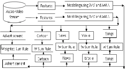
In this paper, evidence from audio and video are combined for classification using weighted sum rule. This work presents a combining method for audio-video classification. Fig. 1, shows the block diagram of audio and video for and classification using SVM and AANN modeling techniques. The paper is organized as follows. The acoustic and visual feature extractions are presented in Section 4. Modeling technique for audio and video classification is described in Section 5. Experimental results of audio classification, video classification and audio-video based classification are reported in Section 6. Conclusion is given in Section 7.
3.
RELATED WORK
3.1
Audio Classification
Recent study shows that the approach to automatic audio classification uses several features. To classify speech/music element in audio data stream plays an important role in automatic audio classification. The method described in [1] uses SVM and Mel frequency cepstral coefficients, to accomplish multi group audio classification and categorization. The method gives in [11] uses audio classification algorithm that is based on conventional and widely accepted approach namely signal parameters by MFCC followed by GMM classification. In [6] a generic audio classification and segmentation approach for multimedia indexing and retrieval is described. Musical classification of audio signal in cultural style like timber, rhythm, and wavelet confident based musicology feature is explained in [5]. An approach given in [8] uses support vector machine (SVM) for audio scene classification, which classifies audio clips into one of five classes: pure speech, non pure speech, music, environment sound, and silence.
3.2
Video Classification
Automatic video retrieval requires video classification. In [7], surveys of automatic video classification features like text, visual and large variety of combinations of features have been explored. Video database communication widely uses low-level features, such as color histogram, motion and texture. In many existing video data base management systems content-based queries uses low-level features. At the highest level of hierarchy, video database can be categorized into different genres such as cartoon, sports, commercials, news and music and are discussed in [13], [14], and [15]. Video data stream can be classified into various sub categories cartoon, sports, commercial, news and serial are analysis in [2], [3], [7] and [16]. The problems of video genre classification for five classes with a set of visual feature and SVM is used for classification is discussed in [16].
[image:1.595.316.534.188.308.2]
4.
FEATURE EXTRACTION
4.1 Acoustic Feature
Acoustic features representing the audio information can be extracted from the speech signal at the segmental level. The segmental features are the features extracted from short (0 to 5 minutes) segments of the speech signal. These features represent the short-time spectrum of the speech signal. The short-time spectrum envelope of the speech signal is attributed primarily to the shape of the vocal tract. Mel-frequency cepstral coefficients (MFCC) have been commonly used in speech processing. Fig. 2. illustrates the computation of MFCC features for a segment of audio signal which is described as follows:
The computation of MFCC can be divided into five steps.
1. Audio signal is divided into frames.
2. Coefficients are obtained from the Fourier transform.
3. Logarithm is applied to the Fourier coefficients.
4. Fourier coefficients are converted into a perceptually
based spectrum.
5. Discrete cosine transform is performed.
In our experiments Fourier transformation uses a hamming window and the signal should have first order pre-emphasis using a coefficient of 0.97. The frame period is 10 ms, and the window size is 20 ms. to represent the dynamic information of the features, the first and second derivatives, are appended to the original feature vector to form a 39 – dimensional feature
.
Visual Feature
Color histogram is used to compare images in many applications. In this work, RGB (888) color space is quantized into 64 dimensional feature vector, only the dominant top 16 values are used as features. The image/video histogram is a simply bar graph of pixel intensities. The pixels are plotted along the x – axis and the number of occurrences for each intensity represent the y-axis.
p (rk) = nk / n, 0 k L-1 (1)
where
rk – kth gray level
nk – Number of pixels in the image with that gray level
L – Number of levels (16)
n – Total number of pixels in the image
p (rk) – gives the probability of occurrence of gray level rk .
5.
MODELING
TECHNIQUE
FOR
AUDIO AND VIDEO CLASSIFICATION
5.1 Support Vector Machine (SVM) for
Classification
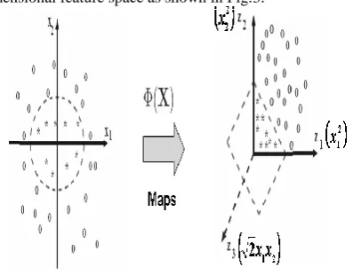
The basic idea is to map the input space to the higher dimensional feature space as shown in Fig.3.
[image:2.595.328.527.172.327.2]Fig.3. Principle of Support Vector machine
Support vector machine (SVM) has been used for classifying the obtained data (Burges, 1998). SVM is a supervised learning method used for classification and regression. They belong to a family of generalized linear classifiers. Let us denote a feature vector (termed as pattern) by x=x1,x2,……xn
and its class label by y such that y = {+1,−1}. Therefore, consider the problem of separating the set of n-training patterns belonging to two classes,
X1
Inputs WN1
.
WN2.
. s O/P
X2 W NS
[image:2.595.59.258.241.329.2]
Fig.4. Architecture of the SVM (Ns is the number of support
vectors).
(xi, yi) , xi R n
, y = {+1, -1}; i = 1, 2…..n (2)
A decision function g (x) that can correctly classify an input pattern x that is not necessarily from the training set.
5.1.1 SVM for Linearly Separable Data
A linear SVM is used to classify data sets which are linearly separable. The SVM linear classifier tries to maximize the margin between the separating hyperplane. The patterns lying on the maximal margins are called support vectors. Such a hyperplane with maximum margin is called maximum margin
K
2(.)
K
Ns(.)
∑
K
1 [image:2.595.313.570.455.599.2](.)
hyperplane [9]. In case of linear SVM, the discriminate function is of the form:
g (x) = w t x + b (3) Such that g ( x i ) ≥ 0 for yi = +1 and g (x i ) < 0 for yi = −1. In
other words, training samples from the two different classes are separated by the hyperplane g (x) = w tx +b = 0. SVM finds the hyperplane that causes the largest separation between the decision function values from the two classes.
Now the total width between two margins is
w
w
w
J
(
)
2
t whichis to be maximized. Mathematically, this hyperplane can be
found by minimizing the following cost function: Subject to separability constraints
J
w
w
tw
2
1
)
(
(4)g (xi) ≥ +1 for yi = +1
or (5) g (xi) ≤ −1 for yi = −1
Equivalently, these constraints can be re-written more compactly as
yi (w t
xi +b) 1 i = 1,2…..n (6)
For the linearly separable case, the decision rules defined by an optimal hyperplane separating the binary decision classes are given in the following equation in terms of the support vectors:
Ns i
i
i i
i
xx
b
y
sign
Y
1
(7)where Y is the outcome, yi is the class value of the training
example xi, and represents the inner product. The vector corresponds to an input and the vectors xi, i = 1. . . . Ns, are
the support vectors. In Eq (6), b and _αi are parameters that
determine the hyper plane.
5.1.2 SVM for Linearly Non-separable Data
For non-linearly separable data, it maps the data in the inputspace into a high dimension pace
x
R
I
x
R
H, with kernel function
(
x
)
to find the separating hyperplane. A high-dimensional version of Eq. (6) is given as follows:
N i
i
i i
i
x
x
b
y
sign
Y
1
,
(8)5.2
Auto Associative Neural Network
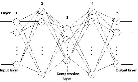
Auto associative neural network models are feed forward neural networks performing an identity mapping of the input space, and are used to capture the distribution of input data. AANN models are used to capture the distribution of the feature vectors for each subject. The distribution capturing ability of the AANN model is described in this section. The five layer auto associative neural network model is used to capture the distribution of extracted level of features. The second and fourth layers of the network have more units than the input layer. The third layer has fewer units than the first or fifth. The activation functions at the second, third and fourth layer are nonlinear.Fig 5(a) A Five Layer AANN model
Let us consider the five layer AANN model shown in Fig.5(a).,which has three hidden layers. The processing units in the first and third hidden layers are non-linear, and the units in the second compression/hidden layer can be linear or non-linear.
Fig5(c) Probability Surface. Fig5(b) Two dimensional output
Fig 5(a) Artificial two dimensional data
Fig. 5. Distribution capturing ability of AANN model
[image:3.595.319.541.72.204.2]In order to visualize the distribution better, one can plot the error for each input data point in the form of same probality surface as shown in Fig. 5 ( c ). The error Ej for the data point
i in input space is plotted as pj= exp (-Ei /α ) , where ∞ is a
constant. Note that pi is not strictly a probability density
function, but we call the resulting surface as probability density function. The plot of the probability surface shown a large amplitude for smaller error Ei , indicating better match of
the network for that data point. The constraints imposed by
thenetwork can be seen by the shape the error surface taken in both the cases. Once can use the probability surface to study
the characteristics of the distribution of the input data capture by the structure of the network, Ideally, one would like to achieve the best probability surface, best defined in terms of same measure corresponding to a low average error.
The five auto associative neural network models as described in section 5.2, are used to capture the distribution of the acoustic and visual feature vectors. The structure of AANN model used in our study is 39L 78N 4N 78N 39L for MFCC, 64L 128N 8N 128N 64L for color histogram, for capturing the distribution of the acoustic and visual features of a class, where l denotes a linear units, and N denotes nonlinear unite. The nonlinear units use is tanh(s) as the activation, where s is the activation value of the unit. The network is trained using back propagation learning algorithm is used to adjust the weights of the network to minimize the mean square error for each feature vector.
6.
EXPERIMENTAL RESULTS
For conducting experiments, audio and video data are recorded using a TV tuner card from various television regional language channel(sun tv, sony tv, star tv, udhya tv, suriya tv and vijay tv) at different timings to ensure quality and quantity of data stream. The training data test includes 6-min of audio stream for each genres, 6-6-min of video stream for each genres. Audio stream is recorded at 8 KHz with mono channel and 16 bits per sample. Video clips are
recorded with a frame resolution of
320
240
pixels and frame rate of 25 frames per second. Training data is segmented into fixed overlapping frames (in our experiments we used 160 ms frames with 80ms overlapping). The sample features extraction process for repeated for audio and video data of varying durations.6.1 Audio and Video Classification using
SVM
Performance of the proposed audio-video classification system is evaluated using the Television broadcast audio database collected from various channels and various genres consists of the following contents: 100 clips of advertisement in different languages, 100 clips of cartoon in different languages, 100 clips on news, 100 clips of movie from different languages, and 100 clips of songs.
Audio samples are of different length, ranging from two min to six min, with a sampling rate of 8 kHz, 16-bits per sample, monophonic and 128 kbps audio bit rate. The waveform audio format is converted into raw values (conversion from binary into ASCII). Silence segments are removed from the audio sequence for further processing 39 MFCC coefficients are extracted for each audio clip as described in Section 4.1. A non-linear support vector classifier is used to discriminate the various categories. The N-class classification problem can be solved using N SVMs. Each SVM separates a c single class from all the remaining classes (one-vs-rest approach).
Support vector machine is trained to distinguish MFCC features of five categories. Support vector machines are
created for each category. The training data finds on optimal way to classify audio frames into their respective classes. The derived support vectors are used to classify audio data. For testing MFCC feature vectors are given as input to SVM model and the distance between each of the feature vector and the hyperplane is obtained. The average distance is calculated for each model. The category of the audio is decided based on the maximum distance. The training data is segmented into fixed-length and overlapping frames (in our experiments we used 20 ms frames with 10 ms frame shift.)
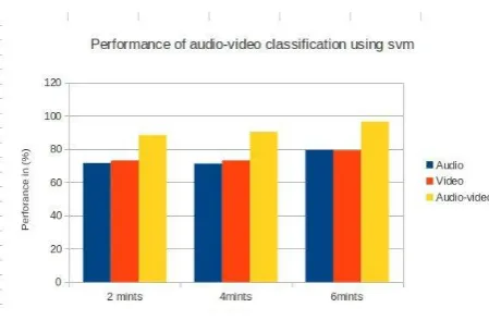
To obtain MFCCs, the audio signals were segmented and windowed into short frames of 100 samples. Magnitude spectrum was computed for each of these frames using fast Fourier transform (FFT) and converted into a set of Mel scale filter bank outputs. Logarithm was applied to the filter bank outputs followed by discrete cosine transformation to obtain the MFCCs. For each audio signal we arrived at 39 features. This number, 39, is computed from the length of the parameterized static vector (13), plus the delta coefficients (13) plus the acceleration coefficients (13). The classification results for the different features are shown in Fig. 3. From the results, we observe that the overall classification accuracy is 77.0 % using MFCC as feature.
Similarly the experiments are conducted using histogram as features in video classification. In our experiment video streams has been recorded and digitized at a resolution of
240
320
pixels and frame rate of 25 frames per second. From television broadcast video data base 6 min video genres stream are taken for training and testing. Each frame will have 64 dimensional vectors in which top 16 values are used as features. Compared to audio classification, video classification is more complicated. The memory used for video classification is twice that used for audio classification. The classification results are shown in Fig. 3. From the results, we observe that the overall classification accuracy is 83.0 % using color histogram as feature.6.2 Combining Audio and Video
Classification using SVM
In this work, combining the modalities has been done at the score level. The methods to combine the two levels of information present in the audio signal and video signal have been proposed. The audio based scores and video based scores are combined for obtaining audio-video based scores as given equation (9). It is shown experimentally that the combined system outperforms the individual system, indicating complementary nature. The weight for each modality is decided empirically.
j j
j
v
p
w
a
n
w
m
(
1
)
,1
j
c
(9)Where
ni j i
j
x
a
1
1
j
c
pi j i
j
y
v
1
j c j i a i
x
ifo th erwise , 1 , 0
n
i
1
,1
j
c
j c j i v i
y
ifo th erwise , 1 , 0
p
i
1
,1
j
c
c i a
-Class label for ith audio frame.
civ -Class label for ith video frame.
v j - Video based score for jth frame.
aj -Audio based score for j th
frame.
mj -Audio-video based score for jth frame.
c -number of classes.
n -number of audio frames.
p -number of video frames.
w -weight.
[image:5.595.54.279.439.586.2]Audio and video frames are combined based on 4:1 ration of frame shifts. The indivual evinces of each audio frame and fourth video frames are combined based on audio and video frames. The weight for each of modality is decided by the parameter w is chosen such that the system gives optimal performance for audio-video based classification. The performance of SVM for audio-video based classification is shown in Fig. 6. This could also be useful for the audio-video indexing and retrieval task.
Fig. 6. Performance of Audio-Video Classification using SVM
6.3 Audio and Video Classification using
AANN
Performance of the proposed audio-video classification system is evaluated using the Television broadcast audio database collected from various channels and various genres consists of the following contents: 100 clips of advertisement in different languages, 100 clips of cartoon in different languages, 100 clips on news, 100 clips of movie from different languages, and 100 clips of songs.
Audio samples are of different length, ranging from one min to five min, with a sampling rate of 8 kHz, 16-bits per sample, monophonic and 128 kbps audio bit rate. The waveform audio format is converted into raw values (conversion from binary into ASCII). Silence segments are removed from the audio
sequence for further processing 39 MFCC coefficients are extracted for each audio clip as described in Section 4.1. A non-linear support vector classifier is used to discriminate the various categories. The training data is segmented into fixed-length and overlapping frames (in our experiments we used 20 ms frames with 10 ms frame shift.)The distribution of 39 dimensional MFCC feature vectors in the feature space and 64 dimensional feature vectors is capture the dimension of feature vectors of each class.
The 39 and 64 dimensional normalized feature vectors are used as input to the AANN model. Feature vectors are extracted 100 samples for each subject for training AANN model. The AANN model is trained using standard back propagation learning algorithm for 100 epochs. The acoustic feature vectors are given as input to the AANN model and the network is trained of 100 epochs. One epoch of training is a single presentation of all training vector.
The training takes about 2 mints on a pc with dual core 2.2 GHz CPU. For evaluating the performance of the system, the feature vector is given as input to each of the model. The output of the input to compute the normalized squared error. The normalized squared error E for the feature vector y is
given by 2
2 || || || 0 -y || y
E
, where 0 is the output vector givenby the model. The error E is transformed into a confidence score c using c=exp (-E). Similarly the experiments are conducted using histogram as features in video classification. In our experiment video streams has been recorded and
digitized at a resolution of
320
240
pixels and frame rate of 25 frames per second. From television broadcast video data base 6 min video genres stream are taken for training and testing. Each frame will have 64 dimensional vectors in which top 16 values are used as features. Compared to audio classification, video classification is more complicated. The memory used for video classification is twice that used for audio classification. The classification results are shown in Table.1. From the results, we observe that the overall classification accuracy is 75.74 % using color histogram as feature and 75.9 % obtained by SVM method.6.4 Combining Audio and Video
Classification using AANN
In this work, combining the modalities has been done at the score level. The methods to combine the two levels of information present in the audio signal and video signal have been proposed. The audio based scores and video based scores are combined for obtaining audio-video based scores as given equation (9). It is shown experimentally that the combined system outperforms the individual system, indicating complementary nature. The weight for each modality is decided empirically.
p i v i n i a iS
p
w
S
n
w
s
1 1)
1
(
1
j
c
(9)Where
n i j i jx
a
1 [image:5.595.318.539.633.753.2]
pi j i
j
y
v
1
1
j
c
j c j
i
a i
x
ifo th erwise ,
1 , 0
n
i
1
,1
j
c
j c j
i
v i
y
ifo th erwise ,
1 , 0
p
i
1
,1
j
c
s -is the combinined audio and video confidence score.
s i a
-is the Confidence score rate of the ith audio frame.
siv -is the Confidence score rate of the ith video frame.
v j - Video based score for jth frame.
aj -Audio based score for jth frame.
mj -Audio-video based score for j th
frame.
c -number of classes.
n -number of audio frames.
p -number of video frames.
w -weight.
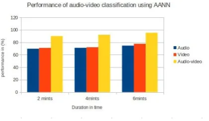
[image:6.595.55.278.74.214.2]The category is decided based on the highest confidence score various from 0 to 1. Audio and video frames are combined based on 4:1 ration of frame shifts. The weight for each of modality is decided by the parameter wis chosen such that the system gives optimal performance for audio-video based classification. The performance of AANN for audio-video based classification is shown in Fig. 7. This could also be useful for the audio-video indexing and retrieval task.
Fig.7 Performance of Audio-Video Classification using AANN
The performance of AANN and SVM for audio-video based classification is shown in Table.1. From the results, we observe that the overall AANN classification accuracy are 72.72 % using color histogram as feature and 72.69 % using MFCC as features.
Table 1 : Combining audio-video classification Results
Audio Video
Audio-Video
AANN 72.55 74.65 93.59
SVM 75.90 75.74 95.54
6. CONCLUSION
This paper proposed an audio-video based classification using SVM and AANN. Mel frequency cepstral coefficients are used as features to characterize audio content. Color Histogram coefficients are used as features to characterize the video content. A non linear support vector machine learning algorithm is applied to obtain the optimal class boundary between the various classes namely advertisement, cartoon, sports, songs by learning from training data. Experimental results show that proposed audio-video classification gives an accuracy of 92.94%., and 95.54%., using AANN and SVM respectively. The results of isolated automatic audio-video classification and indexing. Further experiments have to be conducted automatic audio-video detection and classification using SVM-AANN models for large broad casting programming genres.
7. REFERENCES
[1] Dhanalakshmi. P.; Palanivel. S.; and Ramaligam. V.; (2008), “Classification of audio signals using SVM and RBFNN”, In Elsevier, Expert systems with application, Vol. 36, pp. 6069–6075.
[2] Kalaiselvi Geetha. M.; Palanivel. S.; and Ramaligam. V.; (2008), “A novel block intensity comparison code for video classification and retrivel”, In Elsevier, Expert systems with application, Vol. 36, pp 6415-6420. [3] Kalaiselvi Geetha, M.; Palanivel, S.; and Ramaligam, V.;
(2007), “HMM based video classification using static and dynamic features”, In proceedings of the IEEE international conference on computational intelligence and multimedia applications.
[4] Palanivel. S.; (2004)., “Person authentication using speech, face and visual speech”, Ph.D thesis, I IT, Madras.
[5] Jing Liu.; and Lingyun Xie.; “SVM-based Automatic classification of musical instruments”, IEEE Int’l Conf., Intelligent Computation Technology and Automation (2010.), vol. 3, pp 669–673.
[6] Kiranyaz. S.; Qureshi. A. F.; and Gabbouj. M. ; (2006), “A Generic Audio Classification and Segmentation approach for Multimedia Indexing and Retrieval”., IEEE Trans. Audi., Speech and Lang Processing, Vol.14, No.3, pp. 1062–1081.
[7] Darin Brezeale and Diane J. cook, Fellow. IEEE (2008), “Automatic video classification: A Survey of the literature“, IEEE Transactions on systems, man, and cybernetics-part c: application and reviews, vol. 38, no. 3, pp. 416-430.
[8] Hongchen Jiang. ; Junmei Bai. ; Shuwu .Zhang. ; and BoXu. ; ( 2005),” SVM - based audio scene classification”, Proceeding of NLP-KE, pp. 131–136.
[9] V. Vapnik.;“Statistical Learning Theory”, John Wiley and Sons, New York, 1995.
[10] J.C. Burges Christophe.; “A tutorial on support vector machines for pattern recognition,” Data mining and knowledge discovery, No. 2, pp. 121–167, 1998. [11] Rajapakse. M .; and Wyse. L.; (2005), “Generic audio
[image:6.595.59.270.467.589.2][12] Jarina. R.; Paralici. M.; Kuba. M.; Olajec. J.; Lukan. A.; and Dzurek. M.; “Development of reference platform for generic audio classification development of reference plat from for generic audio classification”, IEEE Computer society, Work shop on Image Analysis for Multimedia Interactive (2008 ), pp-239–242.
[13] Kaabneh,K. ; Abdullah. A.; and Al-Halalemah,A. (2006). , “Video classification using normalized information distance”, In proceedings of the geometric modeling and imaging – new trends (GMAP06) (pp. 34-40).
[14] Suresh. V.; Krishna Mohan. C.; Kumaraswamy. R.; and Yegnanarayana. B.; (2004).,“Combining multiple evidence for video classification”, In IEEE international conference
Intelligent sensing and information processing (ICISIP-05), India (pp.187–192).
[15] Gillespie. W. J.; and Nguyen, D.T (2005).; “Hierarchical decision making scheme for sports video categorization with temporal post processing”, In Proceedings of the IEEE computer society conference on computer vision and pattern recognition (CVPR04) (pp. 908 -913). [16] Suresh. V.; Krishna Mohan. C.; Kumaraswamy. R.; and