http://dx.doi.org/10.4236/ojapps.2015.57033
How to cite this paper: Mylevaganam, S., Srinivasan, R. and Singh, V.P. (2015) Ecohydrologically Driven Catchment Evalua-tion and PrioritizaEvalua-tion. Open Journal of Applied Sciences, 5, 325-334. http://dx.doi.org/10.4236/ojapps.2015.57033
Ecohydrologically Driven Catchment
Evaluation and Prioritization
Sivarajah Mylevaganam1*, Raghavan Srinivasan1, Vijay P. Singh2 1Spatial Sciences Laboratory, Texas A & M University, College Station, TX, USA
2Department of Biological and Agricultural Engineering, Texas A & M University, College Station, TX, USA
Email: *[email protected]
Received 7 June 2015; accepted 12 July 2015; published 15 July 2015
Copyright © 2015 by authors and Scientific Research Publishing Inc.
This work is licensed under the Creative Commons Attribution International License (CC BY).
http://creativecommons.org/licenses/by/4.0/
Abstract
This study develops information based on index, and termed hydro-ecological-index, to represent the need of a riverine ecosystem characterized through a biologically relevant flow regime. The flow regime is defined by a set of parameters, called Indicators of Hydrologic Alteration. These parameters are predicted at the catchment scale by a hydrologic model, called Soil and Water As-sessment Tool. Then the Maximum Entropy Ordered Weighted Averaging method is employed to aggregate non-commensurable biologically relevant flow regimes to develop hydro-ecological- index at the catchment scale. The resulting index reflects the variability of the need of the riverine ecosystem at catchment scale and thus different catchments can be evaluated and compared.
Keywords
Entropy, Principle of Maximum Entropy, Riverine Ecosystem, Indicators of Hydrologic Alteration, Maximum Entropy Ordered Weighted Averaging, Soil and Water Assessment Tool
1. Introduction
One of the objectives of sustainable management of water resources is to meet human needs for freshwater, while maintaining biological diversity, and hydrological and ecological processes essential for the sustenance of the composition, structure, and function of the natural environment that supports life. With the increasing con-cern on riverine ecosystem, many environmental flow assessment methods, such as hydrological rules, hydraulic rating methods, habitat simulation methods, and holistic methodologies [1]-[4] have been applied and modified in response to varying needs. However, by mimicking the natural variability of river flow, the riverine ecosys-tem maintains its variability and remains in good working order which is important for its health. Low flows, for
example, trigger the migration and reproduction within different animal species. On the other hand, high flows, for example, help some riverside plants to reproduce and also ensure that river channels keep their shapes and do not silt up [5] [6]. Thus, since an ecosystem needs flows varying at different times of the year, the above me-thods may not be capable of protecting the future integrity and biodiversity of riverine ecosystems.
It is now recognized that the full range of natural intra- and inter-annual variation of hydrological regimes are critical for sustaining the full native biodiversity and integrity of riverine ecosystems (the “natural flow-regime paradigm”: Indicators of Hydrologic Alteration [5]-[7]). With Indicators of Hydrologic Alteration (IHA), 32 hy-drological statistics/parameters which are assembled into five groups, as shown in Table 1, are calculated for each year of daily streamflow record. These statistics characterize monthly flow variations, the magnitude, fre-quency and timing of high- and low-flow spells, and rates of rise and fall in flow. In other words, a range of flow regime packaged into five groups and 32 hydrological parameters is considered to define the state of the riverine ecosystem such that hydrologic requirements for all aquatic species are met [7].
Amongst the five groups, group-1 includes 12 parameters, and each parameter measures the central tendency (mean) of the daily water conditions for a given month. The 10 parameters in group-2 measure the magnitude of extreme (minimum and maximum) annual water conditions of various durations, ranging from daily to seasonal. Group-3 includes two parameters, the timing of the highest and lowest water conditions within annual cycles. The group-4 parameters include two which measure the number of annual occurrences during which the magni-tude of the water condition exceeds an upper threshold or remains below a lower threshold, and two which measure the mean duration of such high and low pulses. The four parameters included in group-5 measure the number and mean rate of both positive and negative changes in water conditions from one day to the next.
[image:2.595.94.537.522.718.2]Although references [5]-[7] and others emphasize the significance of these 32 biological parameters for representing an ecosystem, the search for a simple tool that transmits technical information in a summarized format, preserving the original meaning of data by using only the variables that best reflect the desired objec-tives, continues. Having information on 32 biological parameters and their values is helpful but does not reflect on parameter dependability and how much each parameter is important for eco-managers. Also, the ability to visualize the 32 dimensions in a spatial context is difficult. Furthermore, the water engineering nomenclature, such as discharge, may not be known to the local people whose real-life experiences can be invaluable for de-vising sustainable water management strategies. On the other hand, the existing functions of riverine ecosystems, as defined by the concerned authorities, may not truly reflect the perceptions of the entire community. Therefore, interactions of all concerned communities may unravel the exact prevailing conditions of the riverine ecosystem. This requires a considerable change in decision making strategies. This means that the results of technical ana-lyses should be presented in a way that can be understood and shared by all stakeholders, including those with little technical background. Therefore, narrowing the result to a single value which could represent the riverine ecosystem would be valuable. The overriding advantage would be that it captures more than one measure in a single number, and allows for quantitative and qualitative elements to be combined.
Table 1. Summary of Hydrological Parameters Used in IHA [7].
Group Characteristics Regime 32 Parameters
Group 1:Magnitude of monthly water conditions Magnitude
Timing Mean value for each calendar month
Group 2:Magnitude and duration of annual extreme water conditions
Magnitude Duration
Annual min/max of 1 day means Annual min/max of 3 day means Annual min/max of 7 day means Annual min/max of 30 day means Annual min/max of 90 day means
Group 3:Timing of annual extreme water conditions Timing Julian date of each annual 1 day minimum and maximum
Group 4:Frequency and duration of high and low pulses Frequency Duration
Number of high and low pulses each year Mean duration of high and low pulses
Group 5: Rate/frequency of consecutive water-condition
changes Rates of Change
Means of all positive differences between daily values Means of all negative differences between daily values
On the other hand, flows are often extremely variable spatially. Flows at locations just a few kilometers apart are sometimes found to be quite different. Therefore, contemporary efforts in planning, designing and imple-menting resource management are at the catchment scale. Having said this, oftentimes the IHA approach is ap-plied at a gage site [7]. However, it is not feasible to establish a flow measuring station on every drainage basin to address the water management at catchment/subwatershed scale.
In recent decades many mathematical models have been developed to understand the hydrological system and provide the simulated data at catchment scale that otherwise would not be measurable [8]-[11]. Some of these models have gained international acceptance as robust interdisciplinary watershed modeling tools, due to their effectiveness in understanding and stimulating important hydrologic phenomena [12]. One such model is Soil and Water Assessment Tool (SWAT). Thus, the objective of this study is to integrate the SWAT prediction at catchment scale with the natural flow-regime paradigm represented by Indicators of Hydrologic Alteration, to develop a hydro-ecological-index that reflects the status of a riverine ecosystem.
2. Soil and Water Assessment Tool (SWAT)
SWAT is a river basin or watershed scale model developed by the United States Department of Agricul-ture(USDA)—Agricultural Research Service(ARS) to predict the impact of land-management practices on water, sediment and agricultural chemical yields in large complex watersheds with varying soils, land use and man-agement conditions over long periods of time [12]. SWAT model operates on a daily time step and predicts wa-ter quality and quantity at subwawa-tershed level. The drainage area is defined by the main outlet. The wawa-tershed is then subdivided into subwatersheds. The modeler can define as many or as few subwatersheds as desired ac-cording to the level of spatial resolution that is reasonable. Each subwatershed is then further divided into a number of hydrologic representative units (HRUs) based on unique combinations of land use and land cover (LULC), soil types and slope within the subwatershed. These HRUs are not spatially defined within the subwa-tershed; they are simply accounting categories which represent the total area of the unique LULC, soil type and slope they represent within a subwatershed. A subwatershed contains at least one HRU, a tributary channel and a main channel or reach. Loads from a subwatershed enter the channel network in the associated reach segment. HRU-scale processes are simulated separately for each HRU and then aggregated up to the subwatershed scale and then routed through the stream system. The details of the model are described by [12].
3. Study Area
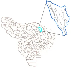
The study area is Kings Creek, a tributary of the Cedar Creek River basin (Figure 1). It has a drainage area of 614 km2 as delineated from a U.S. Geological Survey (USGS) streamflow gaging station (32.513 N, 96.3286 W). Its elevation ranges from 107 m to 190 m and its land use is mainly hay (34%) and range (34.5%). The remain-ing areas were composed of agricultural, forest-deciduous, etc. The average annual precipitation in the study area is 1975 mm.
4. Methodology for Development of Hydro-Ecological-Index
Figure 1. Kings Creek, a Tributary of the Cedar Creek River Basin, Texas.
4.1. Goodness of Fit Criteria
The objective function used in SWAT was to minimize the average Root Mean Square Error (RMSE) of the ob-served vs. simulated flows. The RMSE was defined as:
(
)
2 0.5, , 1
1 RMSE
n
obs i sim i i
Q Q n =
= −
∑
(1)where n is the number of time steps, Qobs,i is the observed streamflow at time i, and Qsim,i is the simulated streamflow at time i. The Nash-Sutcliffe model efficiency (NSE) was used to evaluate SWAT’s overall perfor-mance during calibration and validation. The NSE was defined as:
(
)
(
)
2
, ,
1
2 ,
1
NSE 1
n
obs i sim i i
n
obs i obs i
Q Q
Q Q
=
=
−
= −
−
∑
∑
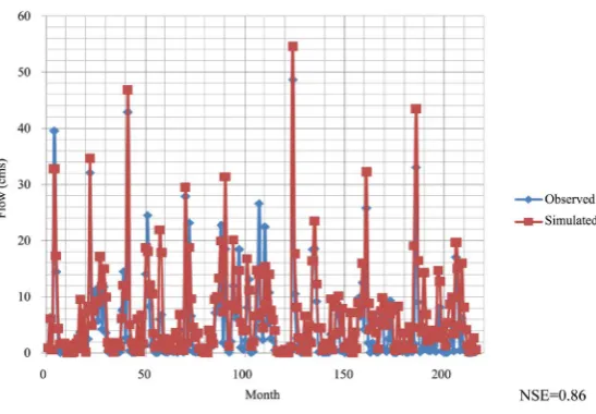
(2)After many trials, a good agreement between observed and simulated flows was obtained as indicated by the NSE of 0.86. Figure 2 shows the model prediction. Model validation was done using the calibrated parameters. Model validation involved re-running the model using input data independent of data used in calibration. Three years of observed flow data from 01 January 1984 to 31 December 1986 were used to validate the model. The validation process led to an NSE of 0.81. This showed a good agreement between measured and simulated flows.
4.2. Determination of IHA Parameters
Figure 2. Observed and Simulated Flow for the Calibration Period.
4.3. Determination of Probability Distributions of IHA Parameters
It was hypothesized that each of the 32 biologically relevant hydrologic parameters, proposed by reference [7], could be considered as a random variable. Then, for each parameter, the least biased probability distribution was obtained by maximizing the Shannon entropy [13]:
1
log N
i i
i
E p p
=
= −
∑
(3)in accord with the Principle of Maximum Entropy (POME), subject to known constraints. In Equation (3) E is the Shannon entropy, p p1, 2,,pN are the values of probabilities corresponding to the specific values
, 1, 2, , ,
i
x i= N of the biologically relevant hydrologic parameter X, and N is the number of values. These probabilities constitute the probability distribution P=
{
p p1, 2,,pN}
of the parameter X:{
x ii, =1, 2,,N}
in question. For maximization, the constraints on X can be expressed in terms of averages or expected values of the parameter reflecting the state of the riverine ecosystem as
( )
1
, 1, 2, ,
N
i j i j
i
p g x C j m
=
= =
∑
(4)1
1, 0, 1, 2, ,
N
i i
i
p p i N
=
= ≥ =
∑
(5)where Cjis the j-th constraint, m is the number of constraints, and gj
( )
xi is the j-th function of x. Using the method of Lagrange multipliers, the maximization of E would lead to the least biased P expressed as [13]:( )
0 1
exp , 1, 2, ,
m
i j j i
j
p λ λ g x i N
=
= − − =
∑
(6)In practical applications, functions gj
( )
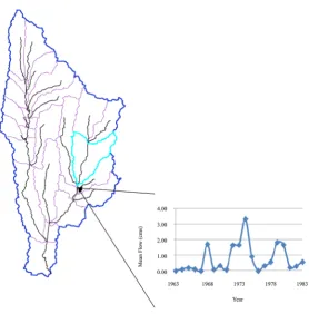
xi are expressed as simple moments and the number of constraint iskept to two or three. Thus, the first constraint would be the average and the second constraint would be the second moment or variance. Once the least biased probability distribution is determined by using Equation (6), it is inserted in Equation (3) to obtain the maximum entropy. This process was carried out for each of the IHA pa-rameters and for each catchment as shown in Figure 3.
To illustrate the method, consider the condition at one of the catchment outlets for one of the IHA parameters, mean flow for the month of January, shown in Figure 4. The constraints on this parameter are expressed in terms of two simple moments: Mean = 0.7421; SD = 0.8882. Using these values, Equations (4) to (5) yield val-ues of Lagrange multipliers as: λ0, λ1,and λ2 [1.1494, −0.9405, 0.6337]. Substitution of these values in Equation
Figure 3. Determination of Maximum Entropy at Catchment Scale.
[image:6.595.173.452.424.707.2]( )
(
2)
2 1exp where 0.7421; 0.8882
2 2
x a
f x a b
b b
− −
= = =
Π (7)
In this manner, the least-biased probability distributions were determined for IHA parameters for all the cat-chments. For most of the parameters, the first two moments and hence the normal probability distribution suf-ficed, providing the maximum entropy values. For group-2 parameters which define the magnitude and duration of the ecosystem, the constraints were specified to log-normal distribution.
4.4. Computation of Maximum Entropy Values
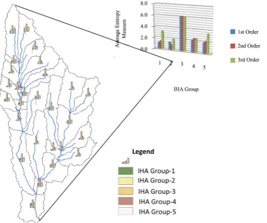
The maximum entropy values were computed from Equation (3) using the least biased probability distributions derived in section 4.3 for each of the biologically relevant parameters and for all the catchments. At the consi-dered catchment outlet, the insertion of the probability distribution in Equation (3) gives the maximum entropy of 1.3006 for the mean flow for the month of January. As shown in Figure 5, the average entropy measure of group-3 is very high compared to the average entropy measure of the remaining IHA groups. This makes it clear that the timing of the highest and lowest water conditions within annual cycles, which provide another measure of life cycle phases (e.g., reproduction), environmental disturbance or stress, heavily defines the underlying ri-verine ecosystem in this study area. In other words, these inter-annual variations in the timing of extreme events reflect that environmental contingency is very high as the entropy measure is high compared to the rest of the IHA groups.
Thus far, it has been shown how to encapsulate the information hidden within each of the 32 biological para-meters through entropy measures. This yields an array
(
E E E1, 2, 3,,E32)
of entropy/information measure ofthe 32 parameters. However, it is reasonable to say that these 32 parameters may have priorities among them-selves. Some of the parameters may not be of importance even though they define the underlying ecosystem. Thus, there has to be a way to consider this with the index development.
4.5. Computation of Hydro-Ecological-Index
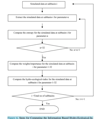
[image:7.595.176.446.475.700.2]Hydro-ecological-index was computed using the steps shown in Figure 6. The values of entropy of biological parameters were aggregated based on [14] such that the final aggregation maximized the information associated with each biological parameter. The Ordered Weighted Averaging (OWA) operator introduced by [14] is a gen-eral type operator that provides flexibility in the aggregation process such that the aggregated value is bounded
Figure 6. Steps for Computing the Information Based Hydro-Ecological-In- dex.
between minimum and maximum values of input parameters. The OWA operator is defined as
(
1)
1 , ,
n n j j
j F a a w b
= =
∑
(8)
where the computed value of entropy for each of the 32 parameters is the argument (ai), bjis the jth largest of ai, and wj are a collection of weights such that wj € [0,1] and
∑
wj=1. Hydro-ecological-index can also be ex-pressed as(
)
(
)
321 32 1 max 2 max 32 max 1
Hydro-ecological-index , , , , , j j
j F a a F E E E E E E w b
=
= = =
∑
(9)The methodology used for obtaining the OWA weighting vector was based on [14]. This approach, which only requires the specification of just the Orness value (1-Andness), generates a class of OWA weights that are called Maximum Entropy Operator Weighted Averaging (ME-OWA) weights. The determination of these weights w1,,w32 from a degree of optimism Orness given by the decision maker requires the solution of an optimization problem formulated below. The objective function used for optimization is one of trying to max-imize the dispersion or entropy, which calculates the weights to be the ones that use as much information as possible about the values of entropy for each of the 32 parameters in the aggregation.
( )
1
log n
i i
i
H W w w
=
= −
∑
(10)subject to:
( )
(
)
1
1 1
n
i i
Orness W n i w
n =
= −
−
∑
(11)1
i w =
∑
where n = 32 and wi∈[ ]
0,1 .The Orness characterizes the degree to which the aggregation is like an “OR” operator. For the analysis an Orness value of 0.75 was assumed in this study to ensure that the impact of all the IHA parameters is considered in the index development and to avoid assigning equal weights as some of the parameters may have more influ-ence on defining the underlying ecosystem. Then, an array of weights wj was generated using Equations (10)
and (11). Using Equation (9), the hydro-ecological-index was found to be [0.3508] for the subwatershed/catch- ment in question. This procedure was followed for the other catchments as well.
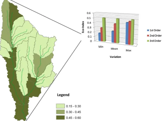
To present the results in a concise way, the eco need of the study area was divided into three categories. As shown in Figure 7, most of the catchments of the study area fall under the lowermost categories. Beside this, the first order streams tend to have a higher variation compared to the streams of 2nd and 3rd order.
5. Conclusions and Recommendations
1) This study outlines an information based on index development to show the eco status of a river basin at catchment scale. It is shown how a hydrological model like SWAT can be used to get an insight about the rive-rineecosystem through natural flow-regime paradigm: Indicators of Hydrologic Alteration. The relative values of the index clearly distinguish the catchments in terms of their needs to sustain the riverine ecosystem. This kind of analysis is significant specifically in ungaged river basins which are dominant in developing countries to define policy towards sustainability.
2) The outlined index development can be extended to analyze the impact associated with river basin activi-ties such as water development projects (e.g., reservoirs, downstream effect of upstream development) and hy-pothetical climate change scenarios. In other words, instead of aggregating the entropy measure at catchment scale, one can aggregate the deviation on entropy measure at catchment scale to reflect the harness level of the system. Such analysis can provide a first insight to spot the critical locations within a river basin.
[image:9.595.173.457.492.701.2]3) For this study, an Orness value of “0.75” is used to develop the hydro-ecological-index. Even though the overall evaluation and prioritization of the 32 parameters should be based on local concerns and local watershed
management goals and objectives, there is a need to evaluate the sensitivity of Orness value on the result. 4) Though the objective of the study is to show how a hydrological model like SWAT can be used to get an insight about the riverine ecosystem through natural flow-regime paradigm: Indicators of Hydrologic Alteration, at catchment scale, it is equally important to have a field reconnaissance and/or monitoring to validate the re-sults.
Acknowledgements
The authors would like to thank Texas Water Resources Institute and U.S. Geological Survey for providing the financial support to conduct this research.
References
[1] Dyson, M., Berkamp, G. and Scanlon, J. (2003) Flow: The Essentials of Environmental Flows, IUCN, Gland,
Switzer-land and Cambridge. http://dx.doi.org/10.2305/IUCN.CH.2003.WANI.2.en
[2] Tharme, R.E. (2003) A Global Perspective on Environmental Flow Assessment: Emerging Trends in the Development
and Application of Environmental Flow Methodologies for Rivers. River Research and Applications, 19, 397-442. http://dx.doi.org/10.1002/rra.736
[3] Naiman, R.J., Bunn, S.E., Nilsson, C., Petts, G.E., Pinay, G. and Thompson, L.C. (2002) Legitimizing Fluvial
Ecosys-tems as Users of Water: An Overview. Environmental Management, 30, 455-467.
http://dx.doi.org/10.1007/s00267-002-2734-3
[4] Postel, S. and Richter, B.D. (2003) Rivers for Life: Managing Water for People and Nature. Island Press, Washington
DC.
[5] Lytle, D.H. and Poff, N.L. (2004) Adaptation to Natural Flow Regimes. Trends in Ecology and Evolution, 19, 94-100.
http://dx.doi.org/10.1016/j.tree.2003.10.002
[6] Poff, N.L., Allan, J.D., Bain, M.B., Karr, J.R., Prestegaard, K.L., Richter, B.D., Sparks, R.E. and Stromberg, J.C. (1997)
The Natural Flow Regime: A Paradigm for River Conservation and Restoration. BioScience, 47, 769-784.
http://dx.doi.org/10.2307/1313099
[7] Richter, B.D., Baumgartner, J.V., Powel, J. and Braun, D.P. (1996) A Method for Assessing Hydrologic Alteration
within Ecosystems. Conservation Biology, 10, 1163-1174. http://dx.doi.org/10.1046/j.1523-1739.1996.10041163.x
[8] Singh, V.P. (1995) Computer Models of Watershed Hydrology. Water Resources Publications, Highlands Ranch, 1130
p.
[9] Singh, V.P. and Frevert, D.K. (2002) Mathematical Models of Small Watershed Hydrology and Applications. Water
Resources Publications, Highlands Ranch, 950 p.
[10] Singh, V.P. and Frevert, D.K. (2002) Mathematical Models of Large Watershed Hydrology. Water Resources
Publica-tions, Highlands Ranch, 891 p.
[11] Singh, V.P. and Frevert, D.K. (2006) Watershed Models. CRC Press, Boca Raton, 653 p.
[12] Gassman, P.W., Reyes, M.R., Green, C.H. and Arnold, J.G. (2007) The Soil and Water Assessment Tool: Historical
Development, Applications, and Future Research Directions. Transactions of the ASABE, 50, 1211-1250.
http://dx.doi.org/10.13031/2013.23637
[13] Singh, V.P. (1998) The Use of Entropy in Hydrology and Water Resources. Hydrological Processes, 11, 587-626.
http://dx.doi.org/10.1002/(SICI)1099-1085(199705)11:6<587::AID-HYP479>3.0.CO;2-P
[14] Yager, R.R. (1999) Induced Ordered Weighted Averaging Operators. IEEE Transactions on Systems, Man and
![Table 1. Summary of Hydrological Parameters Used in IHA [7]](https://thumb-us.123doks.com/thumbv2/123dok_us/8099809.787428/2.595.94.537.522.718/table-summary-hydrological-parameters-used-iha.webp)