A Learning Automata based Algorithm for Solving
Traveling Salesman Problem improved by
Frequency-based Pruning
Mir Mohammad Alipour
Department of Computer Engineering, University of Bonab, Bonab 5551761167, iran
ABSTRACT
Many real world industrial applications involve finding a Hamiltonian path with minimum cost. Some instances that belong to this category are transportation routing problem, scan chain optimization and drilling problem in integrated circuit testing and production. Distributed learning automata, that is a general searching tool and is a solving tool for variety of NP-complete problems, together with 2-opt local search is used to solve the Traveling Salesman Problem (TSP). Two mechanisms named frequency-based pruning strategy (FBPS) and fixed-radius near neighbour (FRNN) 2-opt are used to reduce the high overhead incurred by 2-opt in the DLA algorithm proposed previously. Using FBPS only a subset of promising solutions are proposed to perform 2-opt. Invoking geometric structure, FRNN 2-opt implements efficient 2-opt in a permutation of TSP sequence. Proposed algorithms are tested on a set of TSP benchmark problems and the results show that they are able to reduce computational time, while maintaining the average solution quality at 0.62% from known optimal.
Keywords
Traveling Salesman Problem, Distributed Learning Automata, Frequency-based pruning strategy, Fixed-radius near neighbour.
1.
INTRODUCTION
Traveling Salesman Problem (TSP) is about finding a Hamiltonian path (tour) with minimum cost. TSP is one of the discrete optimization problems which is classified as NP-hard [1]. It is common in areas such as logistics, transportation and semiconductor industries. For instance, finding an optimized scan chains route in integrated chips testing, parcels collection and sending in logistics companies, are some of the potential applications of TSP. Efficient solution to such problems will ensure the tasks are carried out effectively and thus increase productivity. Due to its importance in many industries, TSP is still being studied by researchers from various disciplines and it remains as an important test bed for many newly developed algorithms.
Various techniques have been used to solve TSP. In general, these techniques are classified into two broad categories: exact and approximation algorithms [2]. Exact algorithms are methods which utilize mathematical models whereas approximation algorithms make use of heuristics and iterative improvements as the problem solving process. Some instances in the exact methods category are Branch and Bound, Lagrangian Relaxation and Integer Linear Programming.
Approximation algorithms can be further classified into two groups: constructive heuristics and improvement heuristics.
Instances in constructive heuristics include Nearest Neighbourhood, Greedy Heuristics, Insertion Heuristics [3], Christofides Heuristics [4] etc. Instances in improvement heuristic include k-opt [5], Lin-Kernighan Heuristics [6], Simulated Annealing [7], Tabu Search [8], Evolutionary Algorithms [9-11], Ant Colony Optimization [12,13] and Bee System [14].
In this paper an optimized Distributed Learning Automata (DLA) algorithm is mentioned that significantly improves the computational speed of algorithm proposed previously by the author [15]. Each solution generated by the previous DLA algorithm was locally optimized by an exhaustive 2-opt and proposed algorithm was tested on a set of TSP benchmark instances. The 2-opt heuristic is implemented according to the basic idea which eliminates two arcs in order to obtain two different paths. These two paths are then reconnected in the other possible way if the new path results in a shorter tour length. Although the integration of 2-opt gave promising results, the results presented showed that the execution time could be improved further. To achieve this, two mechanisms, namely FBPS and FRNN 2-opt, are presented in this paper. FBPS is a strategy that allows only a subset of promising solutions to perform 2-opt and FRNN 2-opt is an efficient implementation of 2-opt.
This paper organized as follows: In the next section the Learning Automata and Distributed Learning Automata and 2-opt Local Search Heuristic is introduced and then DLA with 2-opt local search algorithm is described. Section 3 describes FBPS and its working mechanism. In section 4 the FRNN 2-opt adapted from [16] is described. Computational results and findings of this paper are presented and analyzed in section 5 while in the last section conclusions are given.
2.
LEARNING AUTOMATA
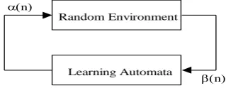
The automaton approach to learning involves determination of an optimal action from a set of allowable actions. An automaton can be regarded as an abstract object that has finite number of actions. It selects an action from its finite set of actions. This action is applied to a random environment. The random environment evaluates the applied action and gives a grade to the selected action of automata. The response from environment is used by automata to select its next action. By continuing this process, the automaton learns to select an action with best response.
The environment can be described by a triple
E
{
,
,
c
}
, where
{
1,
2,...,
r}
represents the finite set of the inputs,
{
1,
2,...,
m}denotes the set of the values canbe taken by the reinforcement signal, and
c
{
c
1,
c
2,...,
c
r}
denotes the set of the penalty probabilities, where the elementi
[image:2.595.87.247.327.389.2]c
is associated with the given action
i. If the penalty probabilities are constant, the random environment is said to be a stationary random environment, and if they vary with time, the environment is called a non stationary environment. The environments depending on the nature of the reinforcement signal
can be classified into P-model, Q-model and S-model. The environments in which the reinforcement signal can only take two binary values 0 and 1 are referred to as P-model environments. Another class of the environment allows a finite number of the values in the interval [0, 1] can be taken by the reinforcement signal. Such an environment is referred to as Q-model environment. In S-model environments, the reinforcement signal lies in the interval [a, b]. The relationship between the learning automaton and its random environment has been shown in Fig. 1.Fig. 1. The relationship between the learning automaton and its random environment.
Learning Automata can be classified into two main families: fixed structure learning automata and variable structure learning automata. A variable structure learning automaton is represented by triple < 𝛼, 𝛽, 𝑇 >, where β is a set of inputs, α is a set of actions and T is learning algorithm. The learning algorithm is a recurrence relation and is used to modify the action probability vector. It is evident that the crucial factor affecting the performance of the variable structure learning automata, is learning algorithm for updating the action probabilities.
Let α(k) and p(k) denote the action chosen at instant k and the action probability vector on which the chosen action is based, respectively. The recurrence equation shown by Eq. (1) and Eq. (2) is a linear learning algorithm by which the action probability vector p is updated. Let ∝𝑖(𝑘) be the action chosen by the automaton at instant k.
𝑝𝑗 𝑛 + 1 = 𝑝 1 − 𝑎 𝑝𝑗 𝑛 + 𝑎 1 − 𝑝𝑗 𝑛 𝑗 = 𝑖
𝑗 𝑛 ∀𝑗 𝑗 ≠ 𝑖 (1)
When the taken action is rewarded by the environment (i.e., 𝛽 𝑛 = 0) and
𝑝𝑗 𝑛 + 1 =
(1 − 𝑏)𝑝𝑗 𝑛 𝑗 = 𝑖
𝑏
𝑟 − 1+ 1 − 𝑏 𝑝𝑗 𝑛 ∀𝑗 𝑗 ≠ 𝑖
(2)
When the taken action is penalized by the environment (i.e., 𝛽 𝑛 = 1). r is the number of actions can be chosen by the automaton, a(k) and b(k) denote the reward and penalty parameters and determine the amount of increases and decreases of the action probabilities, respectively.
If a(k) = b(k), the recurrence equations (1) and (2) are called linear reward-penalty (
L
RP) algorithm, if a(k) >> b(k) the given equations are called linear reward-ε penalty (P R
L
),and finally if b(k) = 0 they are called linear reward-Inaction (
L
RI). In the latter case, the action probability vectorsremain unchanged when the taken action is penalized by the environment.
Learning automata have been found to be useful in systems where incomplete information about the environment, wherein the system operates, exists. Learning automata are also proved to perform well in dynamic environments. It has been shown that the learning automata are capable of solving the NP-hard problems [23].
2.1
Distributed Learning Automata (DLA)
A DLA is a network of the learning automata which collectively cooperate to solve a particular problem [23]. In DLA the number of actions for any automaton in the network is equal to the number of outgoing edges from that automaton. When an automaton selects one of its actions, another automaton on the other end of edge corresponding to the selected action will be activated. The environment evaluates the applied actions and emits a reinforcement signal to the DLA. The activated learning automata along the chosen path update their action probability vectors on the basis of the reinforcement signal by using the learning schemes. Formally, a DLA can be defined by a quadruple < 𝐴, 𝐸, 𝑇, 𝐴0> where
𝐴 = {𝐴1 , … , 𝐴𝑛} is the set of learning automata, 𝐸 ⊂ 𝐴 × 𝐴 is
the set of the vertices in which vertex 𝑒(𝑖,𝑗 ) corresponds to the action ∝𝑗 of the automaton 𝐴𝑖 , T is the set of learning schemes with which the learning automata update their action probability vectors and 𝐴0 is the root automaton of DLA from which the automaton activation is started. For example in Fig. 2, every automaton has two actions, if automaton 𝐴1 selects action 𝛼1 then automaton 𝐴3 will be activated. The activated automaton 𝐴3 chooses one of its actions which in turn activates one of the automata connected to 𝐴3. At any time only one automaton in the network will be active.
Fig. 2. Distributed learning automata.
2.2
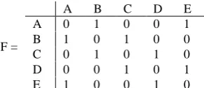
Local Search: 2-OPT Heuristic
The method of 2-opt heuristic is applied frequently to solve TSP. Applying 2-opt heuristic in TSP has some advantages such as simplicity in its implementation and its ability to obtain near optimal results. The basic idea of 2-opt heuristic is to eliminate two arcs in R in order to obtain two different paths. These two paths are then reconnected in the other possible way. Let’s consider a feasible solution, R, with the permutation of “A, B, C, D, E, F, A” with total tour length of 8 units as shown in Fig. 3(a). This closed tour is then further transformed by firstly eliminating two arcs (B, C) and (E, F) and thus producing two separate paths “F, A, B” and “C, D, E”. Next, these two paths are then reconnected to produce another closed tour, R’ = “A, B, E, D, C, F, A”, as shown in Fig. 3(b). Note that there is only one possible way to
Random Environment
Learning Automata n
n
α2
α1
A1
A3
reconnect these two paths in order to preserve the length of the other four arcs. By performing a two-arc transformation, the total length of the closed tour is reduced from 8 units to 6 units. The 2-opt transformation mechanism can be generalized to cater for more arcs in its eliminate-and-reconnect process [5].
Fig. 3. (a) Original closed tour, R. (b) R’ after 2-opt transformation
2.3
DLA Algorithm with 2-opt for TSP
In this section, we describe the DLA-2opt algorithm proposed in [15]. At first a network of learning automata which is isomorphic to the graph of TSP instance is created. In this network each node is a learning automaton and each outgoing edge of this node (connecting this city to other city) is one of the actions of this learning automaton.
At first, one automaton selected (activated) randomly as starting city, then at the each stage, active automaton chooses one of its actions based on its action probability vector and heuristic information (it prefer to choose short edges) according to the probability distribution given in Eq. (4).
) 4 ( } ,..., 2 , 1 : )] , ( [
)] , ( [ | {
1
1 1
r i i
j W p
i j W p p p
P r
i j i j i j i j i
j
where
P
ijis the is the probability with which automaton jchooses to move from city j to city i,
W
1(
j
,
i
)
is the inverse of the distance between city j to city i, i is the one of cities that can be visited by automaton on city j (to make the solution feasible), and
1
is a parameter which determines the relative importance ofP
ijversus distance. In Eq. (1) wemultiply the
P
ijby the corresponding heuristic value)
,
(
1i
j
W
. In this way we favor the choice of edges whichare shorter and which have a greater j
i
P
.This action activates automaton on the other end of edge. The process of choosing an action and activating an automaton is repeated until a tour is created, this means, every node of the graph is visited and coming back at starting city (or making a feasible tour is impossible). In order to exclude loops from the traversed paths, the algorithm meets every node along a path being traversed once (except starting city). To implement this, if an automaton chooses action ∝𝑘 from the list of its actions, then all inactivated automatons (unvisited nodes) will disable action ∝𝑗 in their list of actions. However, at the next iteration of the algorithm, all the disabled actions will be enabled. The action of a DLA is a sequence of actions that represents a particular tour in the graph. After this, the solution is improved by 2-opt heuristic. The outline of our DLA 2-opt algorithm is shown in Fig. 4.
Procedure TSP Begin
Repeat Produce a tour by DLA.
Perform 2-opt on this tour. Compute the tour length.
if CurrentTourLength < BestTourLength then Reward the selected actions of all LAs along the tour according to the
L
RI.Modify the Probability vector.
End if Enable all the disabled actions of each LAs.
Until (stop condition reached) End Procedure
Fig. 4. DLA with 2-opt local search for TSP
The environment uses the length of this tour to produce its response. This response, depending on whether it is favorable or unfavorable, causes the actions along the traversed path be rewarded if it is favorable (the action probability vectors remain unchanged if it is unfavorable) according to linear Reward-Inaction learning algorithm
(
L
RI)
.3.
FREQUENCY-BASED PRUNING
STRATEGY
FBPS is based on building blocks concept that has been found in many areas. One of them is the Genetic Algorithms (GA) in computer science. Gero et al [24,25] studied the building blocks in GA chromosomes. A population of chromosomes is divided into two groups, one above a threshold (better fitness), and the other one below the threshold (lower fitness). They proposed a mechanism to identify prevalent building blocks in the better fitness group and absent building blocks in the lower fitness group. The identified building blocks are then combined as a single gene and they are prevented from further modifications by crossover and mutation. The proposed approach was tested on space layout planning and results showed that if these blocks are frequently reused in the evolutionary process, a significant reduction of computational time can be achieved. The FBPS proposed in this paper is able to identify some common building blocks in the TSP solutions generated by DLAs. The identified building blocks will be used to decide which solutions need to be further improved by 2-opt.
If every solution generated by DLAs locally be optimized using 2-opt, computational time for obtaining good results is highly increased. Hence, a pruning strategy based on the accumulated frequency of building blocks is proposed to prohibit 2-opt operations from being performed on some solutions. Consider the following example that explains the working mechanism of the pruning strategy. Firstly, an n × n matrix is created with each entry of the matrix assigned to zero. n is the number of cities of a TSP instance. If a TSP instance with 5-city is being solved, a matrix 𝐹5∗5 is required:
F =
A B C D E
A 0 0 0 0 0
B 0 0 0 0 0
C 0 0 0 0 0
D 0 0 0 0 0
E 0 0 0 0 0
F is used to record the accumulated frequency of the smallest building blocks of every solutions generated by DLAs. In this case, the smallest building block contains two elements. Consider the solution “A, B, C, D, E, A” and how F will be updated:
1 1 1
1 1
1
D
E B A
C F
(b) (a)
1 1 1
1 1
1
D
E B A
C F
[image:3.595.315.541.69.235.2]F =
A B C D E
A 0 1 0 0 1
B 1 0 1 0 0
C 0 1 0 1 0
D 0 0 1 0 1
E 1 0 0 1 0
In this paper only the smallest edges (edge between two nodes) is considered in a solution, but it can be extended to consider building blocks in different sizes e.g. three-element block and so on. For every building block found in the permutation, two entries of F will be updated. For instance, when the building block AB is encountered, the entries of AB and BA of F are both incremented by 1. Consider another solution “A, B, E, D, C, A” is generated, result is:
F=
A B C D E
A 0 2 1 0 1
B 2 0 1 0 1
C 1 1 0 2 0
D 0 0 2 0 2
E 1 1 0 2 0
Assume the algorithm generates several solutions and then final value of F is as below:
F =
A B C D E
A 0 125 814 32 198
B 125 0 708 382 97
C 814 708 0 30 715
D 32 382 30 0 182
E 198 97 715 182 0
Looking at F, we can identify the building blocks with high frequency. Consider the first row of F as an example, where it records the frequency of the building blocks with A as the first element {AB, AC, AD and AE}. It has a total frequency of 1169 (summation of 125, 814, 32 and 198). The building block of AA is disregarded as the system does not allow any recursive visit. Of these four building blocks, AB contributes 10.69% of the total occurrences ( 1169125 × 100%). AC, AD and AE contribute 69.63%, 2.73% and 16.93% respectively. Rest of entries in F are calculated similarly and the resulting matrix is as below:
F% =
A B C D E
A 0.00 10.69 69.63 2.73 16.93 B 9.52 0.00 53.96 29.11 7.39 C 35.90 31.23 0.00 1.32 31.53
D 5.11 61.02 4.79 0.00 29.07
E 16.61 8.13 59.98 15.26 0.00 Based on F%, building blocks that are q% and above are identified as hot spots. q is a user defined threshold value. For instance, if q = 5%, AB, AC and AE are the hot spots with A as its first element. The identified hot spots will then be employed in the decision making process. The pruning criterion is set as follow: if any solution contains k% or more dissimilar building blocks, it will be prohibited from performing the FRNN 2-opt. Otherwise, it will be further optimized by the FRNN 2-opt. If a permutation of “A, D, C, B, E, A” is considered (based on F% and q = 5%), building blocks of AD and DC are not hot spots. And CB , BE and EA are hot spots. If k is configured at 25%, this particular permutation will be pruned from performing 2-opt. If another permutation of “A, D, E, B, C, A” is encountered, it will be accepted for 2-opt optimization as only one dissimilar building blocks is observed (20% < κ where k is set at 25%). k is a pruning threshold that defined by user and results of tuning it will be mentioned in Section 5.
4.
Fixed-Radius Near Neighbour 2-OPT
In this paper, Fixed-radius Near Neighbour (FRNN) 2-opt is used for efficient implementing 2-opt [16]. The 2-opt swap could not decrease the tour length as both edges increase in length. Because of this observation, the exploration of the second edge can be restricted to a circle centered at a node of the first edge with a radius equal to the edge length.
[image:4.595.99.245.71.134.2]The tour with a permutation of “E, F, I, H, C, G, A, B, D, E” in Fig. 5 will be optimized by 2-opt. While the edge that links E and F, 𝐸𝐸𝐹, serves as the first edge, a search of the second edge based on FRNN method centered at E is performed with a radius of 𝑑𝐸𝐹. All the nodes within the vicinity will be considered to form the second edge together with its single appropriate neighbour. In Fig. 5, node B is found within the vicinity. 𝐸𝐵𝐴 and 𝐸𝐵𝐷 will then be picked as potential candidates for the second edge in 2-opt swap.
Fig. 5. Finding the second edge where 𝑬𝑬𝑭 is the first edge based on FRNN method.
Using FRNN 2-opt, only two comparisons are needed. However, if the exhaustive 2-opt local search is applied on the same permutation of “E, F, I, H, C, G, A, B, D, E” and 𝐸𝐸𝐹 is chosen as the first edge, the potential candidates for second edge are 𝐸𝐼𝐻, 𝐸𝐻𝐶 , 𝐸𝐶𝐺 , 𝐸𝐺𝐴 , 𝐸𝐴𝐵 and 𝐸𝐵𝐷. In the worst case scenario, the exhaustive 2-opt has to perform six comparisons before a successful swap. Considering FRNN 2-opt and exhaustive 2-opt local search, FRNN 2-opt can 67% reduction in terms of the number of comparisons.
5.
EXPERIMENTAL RESULTS
In this section proposed algorithm is tested on a set of benchmark problems taken from TSPLIB1 and some experimental results in this study are presented. The dimension of the problems ranges from 48 to 318 cities. The numerical figure denotes the dimension of the problem. For example, ATT48 is a 48-city problem from the ATT series.
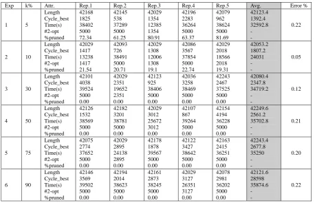
The results for each benchmark instance are computed as an average tour length of five replications. Firstly, results for the experiments of tuning k are presented. Six experiments were carried out with the settings as follows: 𝑎 =2∗(𝑛−2)𝑛∗(𝑛−1) (n is the number of cities) and β = 10. FBPS and FRNN 2-opt is integrated and each experiment consists of five replications. LIN318 (42029 as its known optimal) is used as the test dataset for this set of experiments. The results of the experiments are summarized in Table 1. Whenever a replication achieves the optimum tour length, the execution will be halted and the results will be collected. Otherwise, it will be executed till termination for 5000 iterations (cycles).
1
www.informatik.uni-heidelberg.de/groups/comopt/software/TSPLIB95/
F D
I H C
G A
B
For each replication, the table shows the best tour length, execution time and at which cycle the best tour length is achieved. #2-opt denotes the total number of 2-opt operations if the FRNN 2-opt is performed on every solution.
For cases where the optimum tour length is obtained before 5000 iterations, #2-opt is equal to Cycle_best. For instance, #2-opt for replication 1 in experiment I equals to 1241. For cases where the execution is run for 5000 iterations till termination, #2-opt is equal to 5000. %pruned denotes the total number of pruned solutions and its percentage. In the last column we give the error percentage (%Error), a measure of the quality of the best result found by proposed algorithm (%(Avg - Optimal_Result)/Optimal_Result).
Considering the results shown in Table 1, experiment 2 produces the most satisfactory results. It shows the lowest values for the average tour length and the average computational time, that are 42053.2 and 24031s respectively. In terms of the total number of pruned solutions, Table 1 shows that experiments 3, 4, 5 and 6 fail to prune any solution. This makes their computational times much longer than experiment 2 (nearly 1.5 times of experiment 2), although their average tour lengths are not very much different from experiment 2. In experiment 1, by setting k to a low value, it is expected that the execution time will be reduced. However, the results show otherwise. The FBPS prunes all solutions towards the end of the algorithm execution and this does not contribute to finding the optimal solutions. Hence, more time is needed to search in the space. This makes the performance of experiment 1 not comparable to the rest. All these observations show that k should not be configured either too high or too low. To achieve a reasonable trade off between solution quality and computational cost, k should be set within a bound of [10%, 30%].
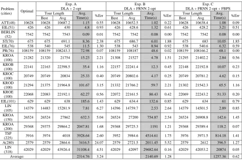
The experimental results that show the performance of the DLA algorithm integrated with FBPS and FRNN 2-opt in terms of solution quality and computational timing on a set of
20 selected problem instances from TSPLIB are presented in Table 2. The table illustrates results of three different sets of experiment. Parameter settings for these three experiments are the same as what were used in previous section, except it will be executed for 10000 iterations. Experiment A uses the 2-opt which requires an exhaustive comparison and swap in its operation. Experiment B uses the FRNN 2-opt, but not the FBPS. Experiment C uses both FRNN 2-opt and FBPS and the k is set at 10%. The results for experiment A in Table 2 has been previously reported in [15] and they were comparable with other seven existing approaches for solving TSP. As the solution quality is maintained after the FRNN 2-opt and FBPS integration, such comparison study as in [15] is not included in this paper. The focus of this paper is to investigate the effect on computational timing when such the integration is made.
As shown in Table 2, the three approaches are able to obtain the optimal or near to optimal tour length for all the problems. Considering all 20 problems together, Table 2 shows that the solution quality is sustained while a major reduction in computational time is observed.
6.
CONCLUSION
[image:5.595.70.529.476.771.2]A new DLA algorithm optimized by frequency-based pruning strategy and efficient implementation of 2-opt has been proposed in this paper. Based on the experimental results, the addition of both FBPS and FRNN 2-opt in the DLA algorithm is able to significantly improve its execution performance compared to the DLA algorithm proposed in [15]. The proposed algorithm will ensure that only a set of promising solutions are locally optimized by FRNN 2-opt, and hence avoid performing an exhaustive 2-opt on every solution generated by DLA.
Table 1: Adjusting k and its Results in experiments.
Table 2: Performance of the DLA Algorithm terms of Solution Quality.
Problem
(cities) Optimal
Exp. A DLA + 2-opt
Exp. B DLA + FRNN 2-opt
Exp. C
DLA + FRNN 2-opt + FBPS Tour Length Avg.
Time(s) %Err
Tour Length Avg.
Time(s) %Err
Tour Length Avg. Time(s) %Err
Best Avg Best Avg Best Avg
ATT(48) 10628 10628 10687.2 1.15 0.55 10628 10652.5 1.02 0.22 10628 10638.4 1.08 0.09 EIL(51) 426 426 430 4.8 0.93 426 428.6 1.32 0.61 426 428.2 3.21 0.51 BERLIN
(52) 7542 7542 7543 0.09 0.01 7542 7542 0.08 0.00 7542 7542 0.08 0.00 ST(70) 675 675 691.1 8.36 2.38 675 686.7 6.01 1.88 675 683 10.05 1.85 EIL(76) 538 540 545 11.5 1.30 538 543 8.94 0.92 538 540.6 6.32 0.59 PR(76) 108159 108159 108243.3 72.98 0.07 108159 108187 48.6 0.02 108159 108166.2 68.1 0.00 KROA
(100) 21282 21320 21754 15.23 2.21 21308 21527 4.78 1.51 21295 21402.2 2.84 0.56 KROB
(100) 22141 22163 22398.5 35.4 1.16 22157 22241.4 12.3 0.45 22148 22192.8 10.07 0.23 KROC
(100) 20749 20749 20834 25.33 0.40 20749 20802.6 4.17 0.25 20749 20781.2 4.62 0.15 KROD
(100) 21294 21375 21964.8 101.67 3.15 21332 21766.2 59.7 2.21 21302 21542.3 65.5 1.16 KROE
(100) 22068 22083 22192.1 62.27 0.56 22072 22161.5 86.43 0.42 22069 22243.2 51.33 0.20 EIL(101) 629 629 638 185.6 1.43 629 634.4 132.6 0.85 629 634 61 0.79
LIN
(105) 14379 14483 15281.9 7.81 6.27 14396 14759.7 2.53 2.64 14379 14501.5 2.89 0.85 KROA
(150) 26524 26524 27862 632.3 5.04 26524 27200 754.87 2.54 26524 26908.8 142.6 1.45 KROA
(200) 29368 29375 29864.2 2047.81 1.68 29368 29725.3 1191 1.21 29368 29389.4 118.2 0.07 TSP
(225) 3916 3974 4018 3928.64 2.60 3952 3984.6 4514.61 1.75 3976 3971.5 814.18 1.41 A(280) 2579 2579 2864.6 3416.5 24.07 2579 2721.5 2011.45 5.52 2579 2612 396.5 1.27
LIN
(318) 42029 42029 43926.4 31108.4 4.51 42029 42097 29682.64 0.16 42029 42053.2 20874 0.05
Average: 2314.76 3.24 2140.69 1.28 1257.36 0.62
7.
REFERENCES
[1] G. Laporte, "The traveling salesman problem: An overview of exact and approximate algorithms," European Journal of Operational Research, vol. 59, no. 2, pp. 231-247, 1992.
[2] G. Laporte, "The traveling salesman problem: An overview of exact and approximate algorithms," European Journal of Operational Research, vol. 59, no. 2, pp. 231-247, 1992.
[3] D. J. Rosenkrantz, R. E. Stearns, and P. M. Lewis, "An analysis of several heuristics for the traveling salesman problem," SIAM Journal on Computing, vol. 6 , no. 3, pp. 563-581, 1977.
[4] A. M. Frieze, "An extension of Christofides heuristic to the k-person travelling salesman problem," Discrete Applied Mathematics, vol. 6, no. 1, pp. 79-83, 1983.
[5] B. Chandra, H. Karloff, and C. Tovey, "New results on the old k-opt algorithm for the traveling salesman problem," SIAM Journal on Computing, vol. 28, no. 6, pp. 1998-2029, 1999.
[6] S. Lin and B. W. Kerninghan, "An effective heuristic algorithm for the traveling salesman problem," Operations Research, vol. 21, no. 2, pp. 498-516, 1973.
[7] E. H. L. Aarts, J. H. M. Korst, and P. J. M. Vanlaarhoven, "A quantitative analysis of the simulated annealing algorithm - A case study for the traveling salesman
problem," Journal of Statistical Physics, vol. 50, no. 1-2, pp. 187-206, 1988.
[8] J. Knox, "Tabu search performance on the symmetric traveling salesman problem," Computers & Operations Research, vol. 21, no. 8, pp. 867-876, 1994.
[9] B. Freisleben and P. Merz, "A genetic local search algorithm for solving symmetric and asymmetric traveling salesman problems," in Proceedings of International Conference on Evolutionary Computation, 1996. pp. 616-621.
[10] P. Merz and B. Freisleben, "Genetic local search for the TSP: New results," in Proceedings of the 1997 IEEE International Conference on Evolutionary Computation, 1997. pp. 159-164.
[11] C. M. White and G. G. Yen, "A hybrid evolutionary algorithm for traveling salesman problem," in Proceedings of Congress on Evolutionary Computation, 2004, CEC2004., 2004. pp. 1473 -1478.
[12] L. M. Gambardella and M. Dorigo, "Solving symmetric and asymmetric TSPs by ant colonies," in Proceedings of IEEE International Conference on Evolutionary Computation, 1996. 1996. pp. 622-627.
[14] P. Lucic and D. Teodorovic, "Computing with Bees: Attacking Complex Transportation Engineering Problems," International Journal on Artificial Intelligence Tools, vol. 12, no. 3, pp. 375-394, 2003.
[15] M. Alipour, "Solving Traveling Salesman Problem Using Distributed Learning Automata improved by 2-opt local search heuristic," Proceedings of First CSUT Conference on Computer, Communication and Information Technology, Computer Science Department, Tabriz University, Tabriz, Iran, pp. 256-264 Nov. 2011.
[16] J. L. Bentley, “Fast algorithms for geometric traveling salesman problems,” ORSA Journal on Computing, vol. 4, no. 4, pp. 387–441, 1992.
[17] K. S. Narendra and K. S. Thathachar, "Learning Automata: An Introduction," (Prentice-Hall, New York, 1989).
[18] M. A. L. Thathachar and P. S. Sastry, "A hierarchical system of learning automata that can learn the globally optimal path," Information Science 42 (1997) 743–766.
[19] M. A. L. Thathachar and B. R. Harita, "Learning automata with changing number of actions," IEEE Trans. Systems, Man, and Cybernetics SMG17 (1987) 1095– 2400.
[20] M. A. L. Thathachar and V. V. Phansalkar, "Convergence of teams and hierarchies of learning
automata in connectionist systems," IEEE Trans. Systems, Man and Cyber-netics 24 (1995) 1459–1469.
[21] S. Lakshmivarahan andM. A. L. Thathachar, "Bounds on the convergence probabilities of learning automata," IEEE Trans. Systems, Man, and Cybernetics, SMC-6 (1976) 756–763.
[22] K. S. Narendra and M. A. L. Thathachar, "On the behavior of a learning automaton in a changing environment with application to telephone traffic routing," IEEE Trans. Systems, Man, and Cybernetics SMC-l0(5) (1980) 262–269.
[23] M. Alipour, "A learning automata based algorithm for solving capacitated vehicle routing problem," International Journal of Computer Science Issues Vol. 9, Issue 2, No 1, pp. 138–145 March 2012.
[24] J. S. Gero and V. A. Kazakov, “Evolving design genes in space layout planning problems,” Artificial Intelligence in Engineering, vol. 12, no. 3, pp. 163–176, 1998. [25] J. S. Gero, V. A. Kazakov, and T. Schnier, “Genetic