Comparative Study between the (BA) Algorithm and (PSO) Algorithm to Train (RBF) Network at Data Classification

Comparative Study between the (BA) Algorithm

and (PSO) Algorithm to Train (RBF) Network at

Data Classification

Ruba Talal

Computer Science Department, Faculty of Computer Science and

Mathematics, Mosul University, Iraq.

ABSTRACT

The Swarm Intelligence Algorithms are (Meta-Heuristic) development Algorithms, which attracted much attention and appeared its ability in the last ten years within many applications such as data mining, scheduling, improve the performance of artificial neural networks (ANN) and classification. In this research was the work of a comparative study between Bat Algorithm (BA) and Particle Swarm Optimization Algorithm (PSO) to train Radial Basis function network (RBF) to classify types of benchmarking data. Results showed that Bat Algorithm (BA) is overcome on (PSO )Algorithm in terms of improving the weights of (RBF) network and accelerate the training time and good convergence of optimal solutions, which led to increase network efficiency and reduce falling mistakes and non-occurrence.

General Terms

Bat Algorithm, Radial Basis Function, Particle Swarm Optimization Algorithm, Neural Network, Classification.

Keywords

RBF, BA, PSO, ANN, Meta-Heuristic.

1.

INTRODUCTION

The Neural Networks is a science that deals with the mathematical methods that can be formulated based on the simulation of biological cells in living organisms, its characterized by neuronal high speed in data processing and by their ability to learn from examples and experiences to produce solutions efficient for complex problems, even in the event that the input incomplete or contain errors [1]. Artificial Neural Networks is a structure of a building parallel information, consisting of units dealing with the handling of information called neurons or elements of the account, which pass signals between neurons across lines linking, and each neuron represents local memory (Local memory) and encloses to each line linking weight (Weight ) hits with a certain numerical signals entering the neuron and then applied to each neuron activation function (Activation Function) on the income of the network, which represents the total income measured signals to determine output signal resulting. artificial neural networks Characterized by ability to perform a variety of tasks, including classification, learning and functions approximation but sometimes practically be performed close to the lower boundary of the solution. Due to the selection of structural inappropriate for the network, or because of the inadequacy of the weights used in the training.

The process of increasing the number of nodes in the hidden layer of the network helps to increase the performance of the network, but some problems can be resolved by using a small number of hidden nodes On the condition of taking the bench optimal network [2]. Unfortunately, the vast majority of neural networks are converging in configuration, and its network of sub-optimal. To address these problems been assumed optimal use two algorithms to improve the performance of artificial neural networks. In this research , the development of the performance of the Radial Basis Function (RBF) network has been improved by using two algorithms and then work a comparison between the performance of two algorithms on the network. Algorithms are random development of roads capable of finding the optimal alternative solutions for traditional methods regular. The linear programming and dynamic programming techniques failed to resolve the complex problems that have a large number of variables and non-linear optical solutions. [2] to overcome these problems, the researchers suggested a number of developmental algorithms for searching near optimal solutions to complex problems. The (PSO) algorithm is inspired by the collective behavior of animals such as flocks of birds, fish and bats [3]. Every solution in the (PSO) algorithm is a bird in the flock and is referred to as a "particle", similar to the chromosome in the genetic algorithm. the process of development (PSO) algorithm is not a process of a new generation of the Son and parent, as is the case in a genetic algorithm but each particle in the community follow the collective behavior and find the best way towards the target. In this research, the application of the two algorithms development bat (BA) algorithm and (PSO)algorithm on the RBF network for improvement of the performance of the network, as was the work of a comparison between the results of two algorithms in terms of the amount of error and standard deviation of benchmarks dataset.

2.

RADIAL BASIS FUNCTION (RBF)

NETWORK

.

.

.

X 2

X n

Q1

Q2

QK

∑

.

.

.

Input Layer Hidden Layer Output Layer

.

.

.

X 1

applied, however, the number of neurons in the hidden layer of RBF network always affects the network complexity and the generalizing capabilities of the network. If the number of neurons of the hidden layer is insufficient, the learning of RBF network fails to correct convergence, however, the neuron number is too high, the resulting over-learning situation may occur. Furthermore, the position of center of the each neuron of hidden layer and the spread parameter of its activation function also affect the network performance considerably. The determination of three parameters that are the number of neuron, the center position of each neuron and its spread parameter of activation function in the hidden layer is very important[7]. The RBF network is consist of two layers except input layer, the hidden layer and output layer, where the network with feed forward and contain two types of training, supervised and unsupervised and its used activation function such as (gaussian function)and the form of the spread data which is similar to radial so called radial basis function network [8]. Several algorithms had been used to train the parameters of the RBF network for classification. The gradient descent (GD) algorithm (1999) is the most popular method for training the RBF network. It is a derivative based optimization algorithm that is used to search for the local minimum of a function [9]. Barreto (2002) used a genetic algorithm, which consists of three operations that are selection, crossover and mutation for training RBF network . The centers of hidden neurons, spread and bias parameters were identified by minimizing the mean square error of the desired outputs and actual outputs [10]. Kurban and Besdok use artificial bee colony algorithm (ABC) to evaluate the weights, spread, bias and center parameters based on the algorithm [11].

2.1

The structure of Radial Basis Function

Neural Network

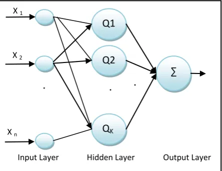
As previously mentioned, a RBFNN consists of three layers: the input layer, the RBF layer (hidden layer) and the output layer. The inputs of hidden layer are the linear combinitions of scalar weights and the input vector x =[x1 , x2 ,…, xn ]T ,

where the scalar weights are usually assigned unity values. Thus the whole input vector appears to each neuron in the hidden layer. The incoming vectors are mapping by the radial basis functions in each hidden node. The output layer yields a vector y = [y1, y2 ,…, ym] for m outputs by linear combination

of the outputs of the hidden nodes to produce the final output.(see Fig. 1) presents the structure of output RBF[12] .

Fig 1: structure of Radial Basis Function( RBFNN)

the network output can be obtained by [12]:

𝑦 = 𝑓 𝑥 = 𝑘𝑖=1𝑤 ∅𝑖 𝑥 + 𝛽𝑖 (1)

where f(x) is the final output, φi (⋅) denotes the radial basis

function of the i-th hidden node, wi denotes the

hidden-to-output weight corresponding to the i-th hidden node, and k is the total number of hidden nodes.

A radial basis function is a multidimensional function that describes the distance between a given input vector and a pre-defined center vector. There are different types of radial basis function. A normalized Gaussian function usually used as the radial basis function, that is[12]

∅𝑖 𝑥 = exp[| 𝑥−𝜇 𝑖 |2_2𝜎𝑖2 ] (2)

where αi and σi denote the center and spread width of the i-th

node, respectively. Generally, the RBFNN training can be divided into two stages[12]:

1. Determine the parameters of radial basis functions, i.e., Gaussian center and spread width. In general, k-means clustering method was commonly used here.

2. Determine the output weight w by supervised learning method. Usually Least-Mean-Square (LMS) or Recursive Least-Square (RLS) was used.

The first stage is very crucial, since the number and location of centers in the hidden layer will influence the performance of the RBFNN directly. The hidden layer of an RBFNN acts as a receptive field operating on the input data space. The number of hidden node based on the distribution of the training data set. The proposed approach performs this task by defining a cluster distance factor, ε , which is the maximum distance between an input sample and a specific RBF node center and allowing the number of basis function to increase iteratively according to this factor[12].

The rationale of this learning is described as follows: the hidden layer starts with no hidden node and ε is pre-determined by PSO to control the clusters production. The first RBF node center α1 is set by choosing one data, x1,

randomly from NT input data sample. The value of Euclidean

2-norm distance between α1 and the next input sample, x2, is

compared with ε . If it is greater, a new cluster whose center location is x2 is created as μ2 ; otherwise, the elements of μ1

are updated as[12]:

𝜇1𝑖 𝑛𝑒𝑤 = 𝜇1𝑖 𝑜𝑙𝑑 + 𝛼 𝑥2𝑖− 𝜇1𝑖 𝑜𝑙𝑑 , 𝑖 = 1,2, . . , 𝑁 3

where α1i and x2i are the i-th component of vectors μ1 and x2,

respectively, || ⋅ || denotes the Euclidean distance and 0 < α < 1 is the updating ratio. Thus, this procedure is carried out on the remaining training samples. The number of clusters grows or RBF nodes center self-adjust continuously until all of the samples are processed. For L clusters, a global spread width σ can be derived by the average of Euclidean distance between each cluster center and its nearest neighbor as[12]:

= µ𝑖− µ𝑗  (4)

where⋅ denotes the expression for the average value for 1 ≤ i ≤ L , 1≤ j ≤ L and i ≠ j . the cluster distance factor , ε ∈ (0, ∞ ) , is obviously a critical factor to determine input space partitioning and obtains the hidden node number and locations in RBFNN. An unduly large value of ε does not reflect an enough number of cluster so it may cause a poor-generalized precision solution. On the contrary, an unduly small value of ε will create redundant clusters; therefore, it may cause overlap

between RBF neurons; moreover, it may lead to poor accuracy and slow convergence either[12].

3.

PARTICLE SWARM OPTIMIZATION

(PSO)

This algorithm is based on the work of Population where the simulated natural behavior flocks of birds in the software program. Is initially create individuals by random and called (Particles). each particle is associated with Velocity. particles is Flying in the search space and is adjusted speed own continuously by the behaviors own a swarm so the particles have a tendency to fly towards the best solution in the search space. Each particle in swarm has the following characteristics:

Xi: is the current location of the particle.

Vi: the current Velocity of the particle.

Pbesti: best position taken by the particle.

Suppose that ƒ represent function quality that measure how close the solution to the optimal solution and t is the current time, the best position taken by the particle is updated as follows: [13]

𝑃𝑏𝑒𝑠𝑡𝑖 𝑡 + 1

= 𝑃𝑏𝑒𝑠𝑡𝑖 𝑡 if 𝑓 𝑥𝑖 𝑡 + 1 ≥ 𝑓(𝑃𝑏𝑒𝑠𝑡𝑖 𝑡 ) 𝑥𝑖 𝑡 + 1 if 𝑓 𝑥𝑖 𝑡 + 1 < 𝑓(𝑃𝑏𝑒𝑠𝑡𝑖 𝑡 )

(5)

The best position in the swarm Gbest (t) at time t is calculated as in equation [13] (2):

𝐺𝑏𝑒𝑠𝑡 t ∈ 𝑃𝑏𝑒𝑠𝑡𝑜 𝑡 , … , 𝑃𝑏𝑒𝑠𝑡𝑛𝑠 𝑡 |𝑓 𝐺𝑏𝑒𝑠𝑡 t

= 𝑚𝑖𝑛 𝑓 𝑃𝑏𝑒𝑠𝑡𝑜 𝑡 , … , 𝑓 𝑃𝑏𝑒𝑠𝑡𝑛𝑠 𝑡 (6)

ns: represents the number of elements in swarm.

The velocity is calculated as the element in the equation(3):

[13]

𝑉𝑖𝑗 𝑡 + 1 = 𝑊 𝑉𝑖𝑗 𝑡 + 𝑐1 𝑟1𝑗 𝑡 𝑃𝑏𝑒𝑠𝑡𝑖𝑗 𝑡 − 𝑋𝑖𝑗 𝑡 +

𝑐2 𝑟2𝑗 𝑡 𝐺𝑏𝑒𝑠𝑡𝑗 𝑡 −𝑋𝑖𝑗 𝑡 7

𝑉𝑖𝑗 𝑡 : represents the velocity of the element i in dimension j

and j is the (j = 1, ..., nx) at time t.

i : represents the position particle and {i = 1,2, .... n}, where n represents the number of birds in swarm.

j {j = 1,2, ..., m} where m represents the dimensions of the problem.

W : represents the weight of inertial value of {0,1}.

𝑋𝑖𝑗 𝑡 ∶ represents the location of the item i in dimension j at

time t.

c1, c2 : represent constants and denote the acceleration coefficients .

𝑟1𝑖 , 𝑟2𝑗 ∶ represent random values in the range (0,1) are taken

from Regular distribution, and these values add random to the algorithm.

Pbest ij (t) : represent the best local location visited element

since i first time.

Finally, particle is updated position i in xi by the following

equation[13]:

Xi (t + 1 ) = Xi (t) + Vi ( t + 1 ) (8)

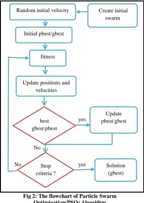
(see Fig.2) represents a flowchart of the algorithm (PSO). were selected the item with the best fitness function for every element, and then to be represented Gbest,then the velocity

element is calculated according to the equation(3),and updated location of the item, according to equation (4). Where they are conducting the following steps repeatedly until the maximum of the iterations within the algorithm or be achieved conditions stop-and-thus is obtain the best solution .

Fig 2: The flowchart of Particle Swarm Optimization(PSO) Algorithm

3.1

The use of (PSO) algorithm to improve

the RBF network

In this paper has been applied (PSO) algorithm to improve the RBF network in terms of the weights (w) and centers (μ) and the structure of the network in addition to the learning the network and to exploit the efficiency of the (PSO) algorithm to improve the training RBF network. Every solution in(PSO) algorithm called (bird) or particle moving in solution space to search for the optimal solution. birds or particles evaluated using the (fitness function) and also called target function or mean squared error (MSE) to search for value appropriate to factor Euclidean distance () used in the training RBF network and evaluate the difference between real output(Yn) and the desired output(Tn). Equation(9) represents the objective function of n samples:

𝑓 𝜀, 𝑦𝑛 = 𝑀𝑆𝐸 𝑦 =

𝑇𝑗𝑘−𝑌𝑗𝑘 2 𝑚

𝑘=1 𝑛 𝑗 =1

𝑛𝑚 (9)

Stop criteria ? Random initial velocity

Initial pbest/gbest

fitness

Update positions and velocities

best gbest/pbest

Create initial swarm

Update pbest/gbest

Solution (gbest) yes

yes No

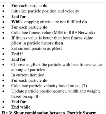
The centers and the width represent as particles and then initialize their own values by K-means algorithm but the values of the weights and the bias are created randomly. Updated bird or particle through equation (7) and (8). The value of the fitness of each bird (particle) which is the value of the error function and evaluated according to the current location of the bird and its velocity of the bird in that location of where (the center, weight, width and b). (see Fig. 3) shows the steps PSO algorithm to train RBF network:

 For each particle do

 initialize particle position and velocity

 End for

 While stopping criteria are not fulfilled do

 For each particle do

 Calculate fitness value (MSE in RBF Network)

 If fitness value is better than best fitness value pBest in particle history then

 Set current position as pBest

 End if

 End for

 Choose as gBest the particle with best fitness value among all particles

 In current iteration

 For each particle do

 Calculate particle velocity based on eq. (7)

 Update particle position(center, width and weight) based on eq. (8)

 End for

 End while

Fig 3: Show combination between Particle Swarm Optimization(PSO) Algorithm and Radial basis function

As mentioned previously that path of each particle in the swarm of birds affected by the path of the best particle in swarm as attracted each particle swarm quickly and at one time to the best particle in the search space, but there is a problem which is to be the best particle in swarm away from the optimal solution as it all starts swarm gather around [13] and it becomes impossible for swarm discovered other areas in the search space so you will blockading swarm is located in a problem and one of the disadvantages of this algorithm, swarm of birds that depend on the particle best in local optima. There is other algorithm called (BAT Algorithm) that mimic the behavior of echolocation by flying bat, causing it to attract the attention of many researchers. (BA) algorithm Based on the frequency tuning and dynamic control of exploration and exploitation, so that the automatic switching to exploration intensive if necessary, in addition to it's similarity (PSO) algorithm in terms of the modified velocities and locations of bats and thus create balanced combination between the PSO algorithm and the local search intensive, which controls the loudness and pulse rate [14].

4.

BAT ALGORITHM (BA)

Bat algorithm (BA) is a meta-heuristic optimization algorithm which was presented by Yang [14]. This algorithm is inspired from the echolocation behavior of microbats. In echolocation behavior, each pulse only lasts a few thousandths of a second (up to about 8–10 ms). Nevertheless, it has a constant frequency which is usually in the range of 25–150 kHz corresponding to the wavelengths of 2–14 mm. Echolocation works as a type of sonar: bats, mainly micro-bats, emit a loud and short pulse of sound, wait it hits into an object and, after a fraction of time, the echo returns back to their ears. Thus, bats can compute how far they are from an object. In addition, this

amazing orientation mechanism makes bats being able to distinguish the difference between an obstacle and a prey, allowing them to hunt even in complete darkness[15]. Yang has idealized the following rules to model Bat algorithm[16]:

1. All bats use echolocation to sense distance, and they also “know” the difference between food/prey and background barriers in some magical way.

2. A bat 𝑏𝑖 fly randomly with velocity 𝑣𝑖 at position 𝑥𝑖

with a fixed frequency 𝑓min, varying wavelength 𝜆

and loudness 𝐴0 to search for prey. They can

automatically adjust the wavelength (or frequency) of their emitted pulses and adjust the rate of pulse emission 𝑟 ∈ [0, 1], depending on the proximity of their target .

3. Although the loudness can vary in many ways, Yang [14] assume that the loudness varies from a large (positive) 𝐴0 to a minimum constant value 𝐴𝑚𝑖

.

Firstly, the initial position 𝑥𝑖, velocity 𝑣𝑖 and frequency 𝑓𝑖 are initialized for each bat 𝑏𝑖. For each time step 𝑡, being 𝑇 the maximum number of iterations, the movement of the virtual bats is given by updating their velocity and position using Equations 10, 11 and 12, as follows:

𝑓𝑖 = 𝑓𝑚𝑖𝑛 + ß 𝑓𝑚𝑎𝑥 – 𝑓𝑚𝑖𝑛 (10)

v𝑖𝑡= v 𝑖𝑡−1+ f𝑖 x𝑖𝑡−1− xcgbest (11)

𝑥𝑖𝑡= 𝑥𝑖𝑡−1+ 𝑣𝑖𝑡 (12)

where 𝛽 denotes a randomly generated number within the interval [0, 1]. Recall that 𝒙𝒊𝒕 denotes the value of decision

variable 𝑗 for bat 𝑖 at time step 𝑡. The result of 𝑓𝑖 (Equation 10) is used to control the pace and range of the movement of the bats. The variable xcgbest represents the current global best

location (solution) for decision variable 𝑗, which is achieved comparing all the solutions provided by the 𝑚 bats. In order to improve the variability of the possible solutions, Yang [14] has proposed to employ random walks. Primarily, one solution is selected among the current best solutions, and then the random walk is applied in order to generate a new solution for each bat that accepts the condition By the following equation:

𝑥new = xold + €Ᾱ(t) (13)

in which Ᾱ (𝑡) stands for the average loudness of all the bats at time 𝑡, and 𝜖 ∈ [−1, 1] attempts to the direction and strength of the random walk. For each iteration of the algorithm, the loudness 𝐴𝑖 and the emission pulse rate 𝑟𝑖 are updated, as follows:

𝐴_𝑖(𝑡 + 1) = 𝛼𝐴𝑖𝑡 (14)

𝑟𝑖𝑡 + 1 = 𝑟𝑖0[1 − 𝑒𝑥𝑝(−𝛾𝑡)] (15)

often randomly chosen. Generally, 𝐴(0) ∈ [1, 2] and 𝑟𝑖(0) ∈ [0, 1] [14].

(see Fig. 4) The steps of bat algorithm (BA) [14]:

 While 𝑡 < 𝑇

 For each bat 𝑏𝑖, do

 Generate new solutions through Equations (10),(11) and (12).

 If 𝑟𝑎𝑛𝑑 > 𝑟𝑖, then

 Select a solution among the best solutions.

 Generate a local solution around the best solution.

 If 𝑟𝑎𝑛𝑑 < 𝐴𝑖 and 𝑓(𝑥𝑖) < 𝑓(xcgbest), then  Accept the new solutions.

 Increase 𝑟𝑖and reduce .

 Rank the bats and find the current best xcgbest.

Fig 4. The steps of bat algorithm

4.1

The use of Bat Algorithm to improve

the Radial basis function network

The process of training RBF network occurs using bat algorithm (BA) by choosing the optimal parameters of the weights between the hidden layer and the layer output (w) and the parameter spread (α) to function mainly in the hidden layer, Centers hidden layer (μ) and bais of the cells in a layer output (𝛽).

The determine number of cells in the hidden layer is very important in RBF network, if the number of cells is few that leads to slow speed of convergence However, if number is a large that leads to the complexity of the network structure, so it was in this paper (1-6 )choose the number of neurons in the hidden layer of the RBF network. The possible solutions are calculated by the fitness function (MSE), which that mentioned earlier. (see Figure 5) shows the (BA) algorithm for training the RBF network, where the algorithm begins to read the data set and then set the required parameters of the RBF network in terms of the number of hidden cells, and the maximum generations . The next step is to determine the parameters controlling of (BA) algorithm.In each generation, every particle evaluated based on a scale MSE as well as dependence on the values of w and μ and ß and α.

 BAT is initializes and passes the best weights to RBF

 Load the training data

 While MSE < Stopping Criteria

 Initialize all BAT Population

 Bat Population finds the best weight and  in Equation 11 and pass it on to the network in Equation 1 and Equation 2.

 RBF neural network runs using the weights and  initialized with BAT

 Bat keeps on calculating the best possible weight,α,ß,µ at each period until the network is converged.

 End While.

Fig 5. Improving Radial Basis Function network by Using Bat Algorithm

5.

COMPARISON BETWEEN (PSO)

ALGORITHM AND (BA) ALGORITHM

FOR TRAINING (RBF) NETWORK

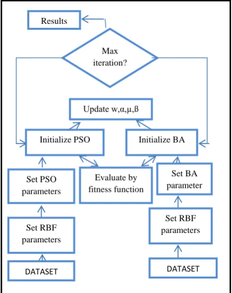
(See Fig.6) shows final structure to comparison between Particle Swarm Optimization (PSO) Algorithm and Bat Algorithm (BA) for training Radial Basis Function (RBF) network. After inserting data set and create the parameters for each of the (RBF) network and (PSO) ,(BA) algorithms to get at the simple structure of the network and accurate results with a minimum of errors and the few execution time .

Fig 6. comparision between (BA) and (PSO)Algorithms for training (RBF) Network

6.

EXPERIMENTAL EVALUATION

In this paper, a comparison between the results of the (PSO) algorithm and the bat algorithm (BA) for training RBF network to classify a set of data taken from the repository UCI [17], which has been used previously by researchers to evaluate the performance of the intelligent algorithms in training neural networks. The program has been implemented in a MATLAB, 2010. The process of selecting parameters for the PSO and BA algorithms plays an important role in the optimization [18]. Because it affects the rate of convergence, in this paper have been identified ideal parameters of PSO and BA algorithms. Through tests and experiments the best weight (w) in PSO algorithm between [0.7,0.8] , c1, c2 = 2, velocity v = 2, the size of the swarm z = 25, the number of iterations 1000. In BA algorithm ,the number of bats N = 20 ,the number of iterations 200 =, fmin = 0, fmax = 1, α = 0.8, γ = 0.7 and L0 = 1, Lmin = 1. from the data set in the repository UCI, has been selected Iris, plant Wine and Glass plant for experiments testing. table 1 shows the standard features of these data.

Results

Max iteration?

Update w,α,µ,ß

Initialize BA Initialize PSO

Evaluate by fitness function

Set BA parameter

s Set PSO

parameters

DATASET

Set RBF parameters

Set RBF parameters

Table 1.shows the standard features of these data

No. of classes No. of

properties No. of

samples dataset

3 4

150 Iris

3 13

178 Wine

7 9

214 Glass

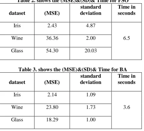
In every execution, the corresponding data set was randomly partitioned in two subsets: training data set (75%), and test data set (25%). Table (2) and (3) illustrate the comparison between the two algorithms in terms of mean square error (MSE) and the standard deviation and the time scale (T) in seconds.

Table 2. shows the (MSE)&(SD)& Time for PSO Time in seconds standard

deviation (

MSE ) dataset

6.5 4.87

2.43 Iris

2.00 36.36

Wine

20.03 54.30

Glass

Table 3. shows the (MSE)&(SD)& Time for BA Time in seconds standard

deviation (

MSE ) dataset

3.6 1.09

2.14 Iris

1.73 23.80

Wine

1.00 18.29

Glass

Table (2) and (3) show that the bat algorithm (BA) is better than (PSO) algorithm in the classification of dataset Iris and Wine and plant Glass and achieve scale error and a standard deviation less than the (PSO) algorithm during a few time of training.

7.

CONCLUSIONS

Through experiments and tests it was concluded that the Bat Algorithm is better than (PSO) Algorithm for training RBF network to classify the benchmarks dataset. Although the PSO algorithm has the power to find a Global Minimum, but its society has a slow rate of convergence in finding from optimal solution, therefore the Bat algorithm is better because its based on the principle of frequency tuning and change the emission rate of impulses which lead to the good affinity from ideal solutions, in addition to the creation process of a balance between exploration and exploitation and accelerate the training time, which led to increase network efficiency and reduce the fall errors and thus the algorithm is very efficient in multiple applications, such as image processing and clustering, which is consider the future recommendations in this paper.

8.

REFERENCES

[1] Dr.laheeb M. Ibrahim, Hanan H. Ali:” Using of Neocognitron Artificial Neural Network To Recognize

handwritten Arabic numbers”. The first scientific conference for information technology - Iraq - Mosul University 22 to 23 December 2008.

[2] Nazri Mohd. Nawi, Abdullah Khan, and Mohammad Zubair Rehman:” A New Back-Propagation Neural Network Optimized with Cuckoo Search Algorithm”. Faculty of Computer Science and Information Technology, Universiti Tun Hussein Onn Malaysia (UTHM).SPRINGER. pp. 413–426, 2013.

[3] Diptam Dutta, Argha Roy, Kaustav Choudhury.” Training Artificial Neural Network using Particle Swarm Optimization Algorithm”. International Journal of Advanced Research in Computer Science and Software Engineering. Volume 3, Issue 3, March 2013.

[4] Horng, M.H. (2010). Performance Evaluation of Multiple Classification of the Ultrasonic Supraspinatus Image by using ML, RBFNN and SVM Classifier, Expert Systems with Applications, 2010, Vol. 37, pp. 4146-4155. [5] Wu, D., Warwick, K., Ma, Z., Gasson, M. N., Burgess, J.

G., Pan, S. & Aziz, T. (2010). A Prediction of Parkinson’s Disease Tremor Onset Using Radial Basis Function Neural Networks, Expert Systems with Applications, Vol .37, pp.2923-2928.

[6] Feng, M.H. & Chou, H.C. (2011). Evolutional RBFNs Prediction Systems Generation in the Applications of Financial Time Seriies Data. Expert Systems with Applications, Vol.38, 8285-8292.

[7] Ming-Huwi Horng, Yun-Xiang Lee, Ming-Chi Lee and Ren-Jean Liou (2012). Firefly Meta-Heuristic Algorithm for Training the Radial Basis Function Network for Data Classification and Disease Diagnosis, Theory and New Applications of Swarm Intelligence, Dr. Rafael Parpinelli (Ed.) 2012.

[8] Ferat , Sahin ,1997, “A Radial Basis function Approach To a color Image Classification Problem in a Real Time Industrial Application”, formerly the scholarty communications projects, Electrical engineering. [9] Karayiannis, N.B. (1999). Reformulated Radial Basis

Function Neural Network Trained by Gradient Descent. IEEE Trnas. Neul Netw., Vol. 3, No, 10, pp. 657-671. [10] Maha Abdul Ilah Mohammed al-Badrani (2008). “The

use of radial basis function network RBFN in the diagnosis of illnesses children”, In Proceedings of the Iraqi Journal of Statiistical Sciences No, 13, pp. 179-195 [11] Kurban T. & Besdok, E. (2009). A Comparison of RBF Neural Network Training Algorithms for Inertial Sensor based Terrain Classification, Sensors, Vol..9, pp. 6312-6329.

[12] Tsung-Ying Sun, Chan-Cheng Liu, Chun-Ling Lin, Sheng-Ta Hsieh and Cheng-Sen Huang.” A Radial Basis Function Neural Network with Adaptive Structure via Particle Swarm Optimization”.

[13] Engelbrecht A. P., (2007):”Computational Intelligence An Introduction”, Second Edition, John Wiley & Sons Ltd, West Sussex, England.

for ptimization (NICSO 2010), Springer Berlin Heidelberg, 2010, pp. 65-74.

[15] D. R. Griffin, F. A. Webster, and C. R. Michael, “The echolocation of flying insects by bats,” Animal Behaviour, vol. 8, no. 34, pp. 141 – 154, 1960.

[16] Gandomi A, Yang X-S, Alavi A, Talatahari S. Bat algorithm for constrained optimization tasks, Neural Computing and Applications, 22(2013) 1239-55.

[17] Blake, C., Keogh, E., Merz, C.J.: UCI Repository of Machine Learning Databases www.ics.uci.edu/ mlearn/MLRepository.html.