6969
FEATURE SELECTION METHODS FOR PREDICTING THE
POPULARITY OF ONLINE NEWS: COMPARATIVE STUDY,
AND A PROPOSED METHOD
1SAMAH OSAMA M. KAMEL, 2MOHAMED NOUR
1Electronics Research Institute, Informatics Research Department, El-Behooth Str., Cairo, Egypt
2Electronics Research Institute, Informatics Research Department, El-Behooth Str., Cairo, Egypt
E-mail: 1[email protected], 2[email protected]
ABSTRACT
Nowadays, accessing the Internet has become interesting for the people’s life. It will be promising if it can accurately predict the popularity of news prior to its publication. Online classification is well suited for learning from large and high dimensional dataset. The main objective of this research work is to predict and evaluate the popularity of online news. Several approaches of feature selection will be adopted to reduce the dataset to improve the classification and prediction accuracy. Some filtering approaches will be used such as correlation, information gain and relief to remove the non-important features so that the classification of new instances will be more accurate. The above mentioned approaches will be presented for selecting the most significant features in the dataset and then providing comparison among their performance. Moreover, Bayes Network and K-Nearest Neighbors algorithms are trained for classification and prediction. The training set is used to construct the models while the testing set is used for validation. This work will be operated and tested using a dataset taken from the UCI machine learning repository containing thousands of articles with sixty-two attributes. A feature selection method is proposed based on features' extraction and/or features' fusion. A comparative study is done among the adopted methods and the novel proposed one. The performance of the adopted classification and prediction models and/or approaches will consider some measurable criteria such as precision, recall, accuracy and error for highlighting the advantages and disadvantages of the adopted approaches and the proposed one. From the experimental work, the performance of the proposed method is promising and outperforms those adopted ones.
Keywords: Feature Selection, Classification Methods, Popularity Prediction, High Dimensional Datasets, and Online News.
1. INTRODUCTION AND RELATED WORK
The process of web contents plays an important role in our life. Web content can be briefly defined as any individual item; in the form of text, audio, video and image; publicity available on a web site. Such items contain a measure that reflects a certain level of interest followed by an online community. Web content is useful in several areas. Examples of such areas are: online marketing, media advertising, economical applications, network dimensioning, predictive problems and others [1]. Identifying the web contents that will be popular is important. Predicting the popularity of web content is an active research area. Several prediction methods for web contents were proposed. This is because the web contents can be broadly defined by any type of information on a web site. The web content improves the subject of the information and the individual item used to define the information [1],[2].
Due to the advances of the Internet, there is an interest in online news which allows fast spread of information around the world. Predicting the popularity of online news is an important trend and it can be measured by the number of interactions in the web and social networks. Predicting the popularity of online news is valuable for authors, advertisers, activists, content providers and others. There are two approaches of popularity prediction. The first one is based on using features only known after publication while the second one doesn’t use such features. The first approach is more common as mentioned in the literature [3], [2]
Moreover, adequate identification of relevant features of a dataset is important. So, it is important to adopt using some of the feature selection methods to reduce the data dimensionality.
6970 Examples of such efforts are briefly mentioned as follows:
[4] the authors discussed the Random Forest regression model which is used to predict popularity of articles from the online news. The authors compared and evaluated the performance of some models with the Random Forest one. The authors also investigated the impact of standardization, correlation and feature selection on some learning models. The work was operated and implemented using a dataset for online news popularity. From the obtained results, the Random Forest model outperforms the other chosen models specifically for the accuracy measure.
[5] the authors mentioned that it would be greatly helpful if it can accurately predict the popularity of news prior to its publication for social media workers. The authors intended to find the best model and set of features to predict the popularity of online news using machine learning techniques. Ten different learning algorithms were implemented on a chosen dataset. The dataset was taken from Mashable; a well-known online news website. The authors used various regression methods, SVM and Random Forest approaches. The performance of the chosen methods/approaches were compared and evaluated. Random Forest was the best one for prediction as it achieved accuracy of 70% with optimal parameters. This is useful to those companies who predict new popularity before publication.
[6] the authors mentioned that the online news is important for spreading awareness of any topic or subject published on the Internet. Online news are available to a large number of users to gather information. The authors used correlation techniques to get the dependency of the popularity obtained from an article and then used genetic algorithm to get the best attributes. The authors implemented twelve learning algorithms on a dataset. The dataset contains about thirty-nine thousands articles with sixty attributes and one decision attribute. The authors presented a comparative study and performance evaluation for the chosen algorithms [6].
[7] the authors mentioned that feature selection is a strategy that can be used to improve categorization accuracy, effectives and computational efficiency. The authors presented a study of some common and useful feature selection methods. This involves term frequency-inverse document frequency (if-idf), information gain, CHI-square (X^2) and symbolic feature selection (SFS). The work was operated using some classifiers such as: Naïve Bayes, K-nearest neighbor, SVM and others. The work was
experimented using Reuters standard dataset. The performance of the adopted feature selection methods and different classifiers were reported.
[8] the authors mentioned that feature selection is a method for removing irrelevant features and reducing dimensionality of the features. The authors proposed a method for selecting the important attributes. The work is concerned with selecting the important attributes and each one is ranked based on the filter and wrapper method. The tree based J48 classifier was used with different test options. Examples of the test options are: 10-fold cross validation using training set, supplying test set and others. Labor dataset was used during the implementation work to test the adopted methods. A comparative study was presented to evaluate the performance of the adopted methods.
[9] the authors discussed the feature selection method based on one-way ANOVA F-test statistics. It was operated to determine the most important features contributing to e-mail spam classification. The adopted feature selection method was applied to reduce the high data dimensionality of the feature space before classification. The experiment was done using spam base benchmarking dataset to evaluate the feasibility of the adopted method. The experimental results showed that the enhanced SVM significantly outperforms SVM and many other recent spam classification methods in terms of complexity and dimension reduction.
This paper implements a comparison among feature selection methods and the novel one using feature fusion and feature selection methods. The performance of the adopted classification and prediction models and approaches illustrates that the advantages and disadvantages of the proposed is better than the adopted approaches. From the experimental work, the performance of the proposed method is promising and outperforms those adopted ones.
6971
2. THE ADOPTED DATASET
To evaluate the performance of the feature selection methods as well as the prediction popularity approaches of online news, the work should be tested using a test bed data collection. The test bed data in our case was chosen from the UCI machine learning repository. That dataset has sixty-two attributes describing different aspects of more than thirty-nine thousands of articles. The attributes of an article involve many aspects such as word, links, digital media, publication time, keywords, natural language processing, target and others. Each aspect has a set of features [5]. Attributes categories are classified into number with integer values, ratios, logic and nominal. The attributes include but not limited to the following: the number of words of the article title, number of links, number of images and videos, number of keywords, worst/best/average keywords, article category, average word length, number of shares, closeness to LDA topics, rate and polarity of positive/negative words, absolute subjectivity/polarity level and others. The last label in the dataset is the class label which is either popular or unpopular.
The articles are classified into six topics. Each topic may be popular or unpopular. Most articles are published on Tuesday, Wednesday, and Thursday respectively. Least articles are published on Weekends. Table 1 shows respectively the articles with their number and percentage for the chosen dataset. For more details, the reader can refer to [5].
Table 1: Articles’ Categories with their Numbers and Percentages
Category No. of Articles percentage %
world 9438 0.23
Technology 8347 0.211
entertainment 8057 0.204
Business 7099 0.180
Social Media 3344 0.084
lifestyle 3100 0.078
3. ANALYSIS OF SOME FEATURE SELECTION METHODS
Feature selection plays an important role in the classification problem. The feature selection process aims at selecting a subset of significant features and discarding others. Feature selection methods are used to reduce the data dimensionality, improve the classification accuracy, and improve the prediction process as well. There are several types of feature selection methods. A brief explanation of some adopted ones is presented as in the following subsections.
3.1 Feature Selection Method based on Correlation
The feature selection method based on correlation aims to analyze the correlation between the data attributes or features of the chosen dataset. Feature selection correlation-based finds and measures correlation on two steps: feature redundancy (intra-feature correlation) and (intra-feature relevancy ((intra-feature- (feature-class correlation) [19]. This method is used to measure the correlation between features as well as between features and classes. It returns the absolute value of correlation as attributes weight. The correlation between features and classes can be briefly written as follows:-
R
∗∗
(1)
Where: Rfc is the correlation between a feature and a class, K is the number of features, Rkc is average of the correlation between features and the class and Rkk is the average linear correlation or inter-correlation between features.
Moreover, the correlation coefficients are used to measure how strong a relationship is between two attributes. Pearson correlation is a correlation coefficient commonly used in regression analysis [17]. The correlation coefficient formula between two features (e.g. x and y) can be presented as follows:-
r ∑ - ∑ ∑ - ∑ ∑∑ - ∑ (2) Where: x is the first feature, y is another feature and n is the sample size.
3.2 Feature Selection Method Based on Information Gain
Information gain is used to measure the importance of features according to the classes in the dataset. The weight of attributes is calculated with respect to the dataset classes. The difference of entropy before and after features appearance in the dataset classes affect on the information gain value. Therefore, the greater weight of attributes gives a greater information gain value. The importance of these attributes in the dataset will affect on the accuracy and error rates [11]. In deeper meaning, attribute subset is obtained with respect to high value of information gain. Equation (3) explains the concept weighted by the information gain.
IG f P c log P c
∣
P f P f ∣∣ c log P f ∣∣ c
∣ ∣
6972 Where: f is a feature of dataset, c is the total number of classes in the dataset, P(ci) is the probability of a class in dataset, P(fp) is the probability of a feature which appears in the dataset, P(fp∣ci) is the probability of appeared feature in class (ci), P(fa) is the probability of a feature which doesn’t appear in the dataset and P(fa∣ci) is the probability of a feature which doesn’t appear in class ci.
3.3 Feature Selection Method Based on Relief
Relief is a statistical filter method. It can deal with nominal and numeric attributes but it’s limited to two classes. Relief is based on weighting each attribute according to its class relevance. Below, the process of Relief is briefly presented [14], [15].
Initially, all weights are set to zero and then updates iteratively. In each iteration, the Relief algorithm chooses a random instance (i) in the dataset and estimates how well each feature value of this instance distinguishes between instances close to (i). In this case, two sets of instances are chosen. Some closest instances are belonging to the same class while others are belonging to a different class. With these instances, the Relief algorithm iteratively updates the weight of each feature. The algorithm differentiates data points from different classes and; at the same time; recognizes data points from the same class. Finally, the features with the highest weights are selected. It is recommended to select only those features with weights above a certain threshold value. The output of the Relief algorithm is a weight between -1 and 1 for each attribute. More predictive attributes can occur for more positive weights.
To update the weight of an attribute, a sample is selected from the data. Identification is done for the nearest neighboring that belongs to the same class; this is called nearest it. Also, identification should be done for the nearest neighboring sample that belongs to the opposite class; this is called nearest miss. A change in attribute value associated with a change in class leads up to weighting of the attribute. This means the attribute change is responsible for the class change. Also, a change in attribute value accompanied by no change in class leads to down weighting of the attribute. This means the attribute change doesn’t have effect on the class. Moreover, updating the weight of the attribute is done for a random set of samples in the data or for every sample in the data. The final weight is then averaged so that the weight becomes in the range [-1, 1] [15], [14].
4. CLASSIFICATION AND PREDICTION APPROACHES
After selecting and implementing the most significant attributes; classification algorithms are applied. The adopted classification algorithms in this work are Bayes Network (BN) and k-Nearest Neighbor (k-NN). It is necessary to build a classification model and test it to measure its performance and to make sure that the selected attributes will improve the performance. Building a prediction model is also important. The logistic regression algorithm is used to predict a new instance which belongs to one of the six topics. It predicts a new instance according to the popularity of online news which may be either popular or unpopular.
4.1.Bayes Network Classification Algorithm
The Bayes Network (BN) is used to represent the joint probability distribution in the discrete, continuous and hybrid environments. The design of BN is based on the number of nodes and edges. Each node represents groups of parents and children which contain large number of random variables whereas edges represent statistical dependencies. The process of the dependence structure of BN can be illustrated briefly as the following sections. It implements the probability conclusion of these variables and calculates the conditional probability of one node and gives certain values of the other nodes. There are two main components of BN structure to implement the process of BN which are a directed acyclic graph (DAG) and a set of conditional probability table (CPT) or a probability density function. First, DAG is used to represent the dependency structure among variables in the network. Second, a set of conditional probability table (CPT) is used for discrete data while a probability density function is used for continuous data [12]. Equation (4) represents the joint probability of the nodes named Chain Rule.
P A ∏ P A |P A (4)
Where: A = {A1, A2, A3, …..,Ai} can be defined as nodes, (A) refers to the joint probability of nodes and Pai(Ai) refers to the parent nodes of Ai which is known as the conditional probability table. Figure 1 shows the process of BN classifier
6973
4.2.k-Nearest Neighbor (k-NN) Classification Algorithm
The k-NN algorithm is used to build a classification model because it is more robust and gives precise results. On the other hand, the k-NN algorithm is lazy as it consumes more time to build the classification model. In this work, the feature selection is an offline phase so time is not important. The implementation of the k-NN algorithm can be simplified in the following steps. First, it converts all features of the dataset into numerical values and all instances are represented as vectors of features in the n-dimensional to decrease the distances among instances. Second, it separates the training dataset into number of classes. The model receives a number of new instances; it predicts each instance according to the nearest neighbors which belongs to their class. The number of the nearest neighbor (k) can be 1 or more. The calculation of the distance between a new instance and its nearest neighbors depends on the usage of the Euclidean Distance Function which can be represented as follows: [13].
𝑓 𝑋 ∑ 𝑥𝑖 𝑦𝑖 (5)
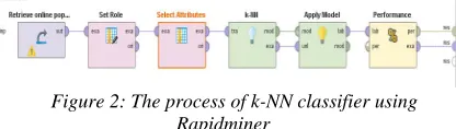
[image:5.612.93.301.424.483.2]Where: k is the number of nearest neighbors, xi is the predicted value, and yi is the value of the nearest-neighbor. Figure 2 shows the Process of k-NN Classifier.
Figure 2: The process of k-NN classifier using Rapidminer
4.3.Analysis of a Regression Model for Predicting Popularity of Online News
The dataset contains six topics as mentioned before; each has two categories: popular and unpopular. The logistic regression approach was adopted to predict the popularity of online news. The idea of regression analysis depends on two types of variables mainly the independent variables and the dependent variable. The independent variables are considered inputs which are known as the predictors. The dependent variable is the output which is called response and it can be either 1 or 0. The idea of regression analysis is crystallized in the relation between the dependent variable and the independent variables and produces the form of the relation between them. When one or more of the independent variables is/are changed while others are fixed, the dependent variable value is changed. The regression approaches may be linear simple regression, linear multiple regression, nonlinear simple regression and nonlinear multiple regression. Due to the nature and
characterization of the chosen dataset, a multiple nonlinear regression method is used (logistic regression). Logistic regression is used to measure the relationship between the response variable (binary dependent variable) and the independent input variables [18]. Figure 3 shows the Process of Logistic Regression.
outcome takes value 1 with probability P 0 with probability 1 P
Logit transform P log (6)
Odds (7)
OR (8)
constant ∗ OR (9)
log constant log OR (10)
Let: log (OR) is BX
log A B X (11)
Equation (12) is logistic function:
logit P y A B X B X ⋯ B X (12)
P y …….. (13)
Where: y is the binary dependent variable {0 or 1},X is independent variables, P(y) is logistic function which shows the probability of the predictors X1, X2,………., Xk, Pi, is the probability of the predictors X1,X2,………, Xk , A is constant and B is the Odd Ratio which is a comparative measure of two odds relative to different variables.
Figure 3: The Process of logistic regression using Rapidminer tool
5. PERFORMANCE METRICS AND DISCUSSION OF RESULTS
5.1.Performance metrics
The performance of the feature selection methods can be evaluated by considering a set of measurable criteria. The criteria or the performance metrics are accuracy, precision, recall, prediction and mean absolute error. Accuracy is evaluated by calculating the correctly classified instances ratio to the total number of instances.
Accuracy (14)
6974 between the true positive (TP) and combination of both true positive and false positive (TP and FP).
Precision (15)
Recall is defined as the ratio between the true positive (TP) and the total number of true positive and false negative (FN)
𝑅𝑒𝑐𝑎𝑙𝑙 (16)
The mean absolute error (MAE) specifies how the predicted values are different from the actual values.
𝑀𝐴𝐸 ∑ |𝐹 𝑌 | ∑ |𝐸 | (17)
Where: Ei is the average of the absolute error Fi is the predicted value and Yi is the actual value.
5.2.Discussion of Results
The first experiment of the feature selection phase uses the correlation matrix to measure the attributes weights and the relation among the features and each other’s as shown in Figure 4. Each feature is related to other features and this relation may be positive, negative or zero. Accordingly, there are strong, medium and weak relations among features.
[image:6.612.314.565.180.452.2]The relationships among features are classified into three types. First, a positive correlation value indicates that there is a strong or medium relationship between features. The range of such correlation value is between 0 < r < 1 (r = 1, 0.9, 0.8, 0.7, ….). The second correlation is no correlation between features where r = 0. The third relationship has negative correlation values which meaning that there is a weak relationship between features.
Figure 4: The relationship among features using the correlation matrix
Using the weighted correlation, every feature is assigned a different weight. According to such weight values some attributes will be chosen for their highly correlated values while others are discarded. Figure 5 presents the weight value associated with each attribute in the dataset.
Figure 5: The weight value for each attribute
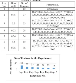
Table 2 shows seven experiments with their features subsets at different threshold values. Figure 6 shows the number of features resulted after applying the seven experiments at the above threshold values.
Table 2: Seven Experiments with their Features Selected Number
Exp. No.
Thre-shold
No. of
Features Features No.
1 0 62 62 features
2 0.15 37
18,27,38,25,16,14,36,41,42,37,17,7,60,3,2 9,40,49,61,10,19,9,48,59,57,46,23,50,8,33
,13,32,28,19,30,39,34,62
3 0.2 33
18,27,38,25,16,14,36,41,42,37,17,7,60,3,2 9,40,49,61,10,19,9,48,59,57,46,23,50,8,33
,13,32,28,62
4 0.22 28 18,27,38,25,16,14,36,41,42,37,17,7,60,3,29,40,49,61,10,19,9,48,59,57,46,23,50,62
5 0.26 24 18,27,38,25,16,14,36,41,42,37,17,7,60,3,29,40,49,61,10,19,9,48,59,62
6 0.3 22 18, 27, 38, 25, 16, 14, 36, 41, 42, 37, 17, 7, 60, 3, 29, 40, 49, 61, 10, 19, 9 and 62
7 0.36 16 18,27,38,25,16,14,36,41,42,37,17,7,60,3,29,62
Figure 6: No. of Features for Experiments
[image:6.612.94.302.460.559.2]Due to the implementation work, Table 3 presents the accuracy (AC %) and error %.
Table 3: Accuracy and Error Rates after Applying BN and k-NN Classification Algorithms
Exp. No.
Thre-shold
No. of Features
AC % of BN
AC % of k-NN
Error % of BN
Error % of k-NN
1 0 62 76.3 87.32 23.7 12.32
2 0.15 37 87.24 86.84 12.76 13.16
3 0.2 33 87.4 86.85 12.5 13.15
4 0.22 28 87.65 86.85 12.35 13.15
5 0.26 24 88.86 88.44 11.14 11.56
6 0.3 22 89.38 89.16 10.62 10.84
[image:6.612.312.568.532.632.2]7 0.36 16 86.1 84.11 13.9 15.89
Figure 7 shows respectively the accuracy % and error rate% w.r.t. the number of features. The precision % and recall % are measured using BN and k-NN classifiers as shown in Table 4. Figure 8 shows respectively precision % and recall % w.r.t. the number of features for the experiments.
62 37
33 28 24 22 16
0 100
Exp. 1Exp. 2Exp. 3Exp. 4Exp. 5Exp. 6Exp. 7
No.
of
F
eatures
Experiment No.
[image:6.612.94.298.633.707.2]6975
Figure 7: Accuracy % and error % after applying BN and k-NN classifiers Table 4: Precision % and Recall % after
Applying BN and k-NN Classifiers
Exp. No.
Thre-shold
No. of Features
Precision % of BN
Precision % of k-NN
Recall % of
BN
Recall % of k-NN
1 0 62 70.6 82.1 71.7 81.8
2 0.15 37 82.23 81.4 82.73 81.62
3 0.2 33 82.6 81.4 82.9 81.6
4 0.22 28 82.92 81.4 83.09 81.5
5 0.26 24 85.08 83.3 84.05 84.1
6 0.3 22 85.85 84.1 84.7 85.3
7 0.36 16 81.4 79.3 81.3 80.2
Figure 8: Precision % and recall % for the seven experiments
From Tables 3 and 4, it is shown that the best values of the performance measures are for that experiment with threshold value equals 0.3. The most important features are reduced to twenty-two features. Due to the implementation of the information gain method, every selected feature is associated with its weight as known in Figure 9. The features subsets are obtained after applying the seven experiments at different threshold values as shown in Table 5.
Figure 9: The features with their associated weights
Table 5: Experiments with their Selected Features’ Numbers
Exp. No.
Thre-shold
No. of
Features Features No.
1 0 62 62 features
2 0.002 37 1,17,18,10,43,45,37,52,21,46,23,38,5,22,61,60,28,27,31,29,42,26,19,30,39, 18,50,7,41,47,13,53,44,1,25,51,62
3 0.0027 32
61,60,28,27,31,29,42,26,19,30,39, 1,17,18,10,43,45,37,52,21,46,23,38,5,22,
18,50,7,41,47,13,62
4 0.003 28 1,17,18,10,43,45,37,52,21,46,23,38,5,22,61,60,28,27,31,29,42,26,19,30,39, 18,50, 62
5 0.0034 24 1,17,18,10,43,45,37,52,21,46,23,38,62 61,60,28,27,31,29,42,26,19,30,39,
6 0.004 20 61,60,28,27,31,29,42,26,19,30,39,1,17,18,10,43,45,37,52,62
7 0.005 18 61,60,28,27,31,29,42,26,19,30,39,1,17,18,10,43,45,62
Figure 10 shows the resulted number of features for the seven experiments. Table 6 shows the accuracy % and error % for BN and k-NN algorithms respectively. Figure 11 shows respectively the accuracy % and error % for each obtained number of features for the seven experiments
.
Figure 10: No. of features for experiments
Table 6: Accuracy % and Error % after Applying BN and k-NN Algorithms
Ex p. No.
Thre-shold Features No. of AC % of
BN
AC % of
k-NN
Error % of BN
Error % of k-NN
1 0 62 76.3 87.32 23.7 12.32
2 0.002 37 85.6 87.23 14.4 12.77
3 0.002 32 87.72 87.3 12.28 12.7
4 0.003 28 88.93 88.2 11.07 11.8
5 0.003 24 89.44 88.8 10.26 11.2
6 0.004 20 89.75 89.1 10.25 10.9
7 0.005 18 89.75 86.4 10.25 13.6
Figure 11: Accuracy % and error % after applying BN and k-NN algorithms respectively
Table 7 shows the results of precision and recall after applying both BN and k-NN algorithms. Figure 12 shows respectively the precision % and recall % w.r.t. the number of features resulted from the experiments.
Table 7: Precision % and Recall% after Applying BN and k-NN Algorithms
Exp.
No. Thre-shold Features No. of Precision % of BN
Precision % of
k-NN
Recall % of
BN
Recall % of k-NN
1 0 62 70.6 82.4 71.7 81.5
6976
3 0.002 32 82.62 82.4 83.4 81.6
4 0.003 28 85.15 83.6 85.67 84.1
5 0.003 24 85.15 83.6 85.67 84.1
6 0.004 20 85.68 84.4 86.04 85.3
7 0.005 18 85.68 81.3 86.04 80.2
Figure 12: Precision % and recall % after applying BN and k-NN algorithms
From Tables 6 and 7, it is noticed that when threshold is increased, the accuracy %, precision % and recall% increase while the error % is decreased. At the threshold value 0.0055, the value of performance metrics is fixed. The most significant features are at threshold value 0.0055. The number of individual features of the dataset was reduced to eighteen features. The third feature selection method is Relief method and the result of this implementation is shown in Figure 13.
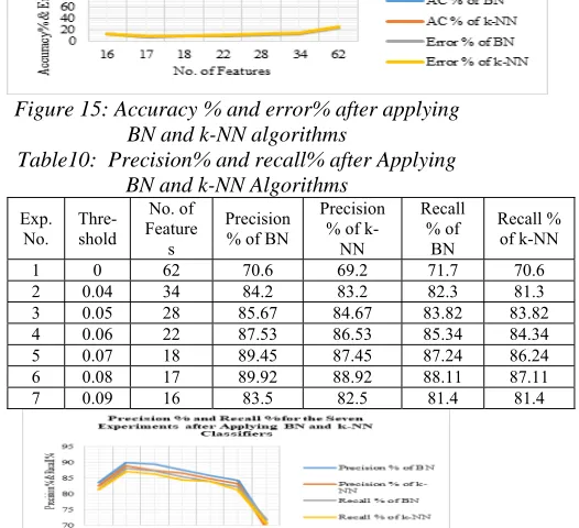
Similarly, the features with their weights, the number of important features for each experiment for its threshold, accuracy %, error %, precision % and recall % are presented respectively in Figures 13 – 16. The details of such parameters are illustrated also in Tables 8 – 10 respectively.
Figure 13: Features with their weights
Table 8: The No. of Experiments and Features Number
Exp. No.
Thre-shold
No. of
Features Features No.
1 0 62 62 features
2 0.04 34
27,42,56,43,16,57,9,25,39,58,59,17,44, 24,3,46,50,7,48,35,49,33,32,45,34,18,5
3,38,12,29,31,36,55,62
3 0.05 28
27,42,56,43,16,57,9,25,39,58,59,17,44, 24,3,46,50,7,48,35,49,33,32,45,34,18,6
2
4 0.06 22 27,42,56,43,16,57,9,25,39,58,59,17,44,24,3,46,50,7,48,35,49,62
5 0.07 18 27,42,56,43,16,57,9,25,39,58,59,17,44,24,3,46,50,62
6 0.08 17 27,42,56,43,16,57,9,25,39,58,59,17,44,24,3,46,62
7 0.09 16 27,42,56,43,16,57,9,25,39,58,59,17,44,24,3,62
[image:8.612.304.567.54.681.2]Figure 14: No. of features for experiments
Table 9: Accuracy % and Error % after Applying BN and k-NN Algorithms
Exp . No.
Thre-shold
No. of Feature
s
AC % of
BN
AC % of
k-NN
Error % of BN
Error % of k-NN
1 0 62 76.3 75.1 23.7 24.9
2 0.04 34 88.1 86.1 11.9 13.9
3 0.05 28 89.04 87.04 10.96 12.96
4 0.06 22 90.27 89.27 9.73 10.73
5 0.07 18 91.63 90.63 8.37 9.37
6 0.08 17 92.1 91.1 7.9 8.9
[image:8.612.91.526.70.232.2]7 0.09 16 87.5 86.4 12.3 13.3
Figure 15: Accuracy % and error% after applying BN and k-NN algorithms
Table10: Precision% and recall% after Applying BN and k-NN Algorithms
Exp. No. Thre-shold
No. of Feature
s
Precision % of BN
Precision % of
k-NN
Recall % of
BN
Recall % of k-NN
1 0 62 70.6 69.2 71.7 70.6
2 0.04 34 84.2 83.2 82.3 81.3
3 0.05 28 85.67 84.67 83.82 83.82
4 0.06 22 87.53 86.53 85.34 84.34
5 0.07 18 89.45 87.45 87.24 86.24
6 0.08 17 89.92 88.92 88.11 87.11
7 0.09 16 83.5 82.5 81.4 81.4
Figure 16: Precision% and recall% after applying BN and k-NN algorithms
[image:8.612.310.573.385.625.2]6977 feature subset was obtained at the threshold value 0.08 which achieved high accuracy and minimum error. The number of features of the dataset was reduced from sixty-two features to seventeen features. The most important features are: 27, 42, 56, 43, 16, 57, 9, 25, 39, 58, 59, 17, 44, 24, 3, 46 and 62.
It is obvious that Relief performance is different from those correlation and information gain methods. The most significant features subset was obtained by using relief method which gives higher accuracy, precision and recall and minimum error. The Relief process is based on number of iterations in order to get the most significant feature subset.
6. A PROPOSED METHOD BASED ON FEATURES' SELECTION AND/OR FUSION
As mentioned before, the prediction of online news popularity is one of the important challenges of enormous amount of news. To improve the classification performance, the useful set of features should be selected. The bad or irrelevant features which don’t provide class separability should be discarded. Irrelevant features are those features that have low correlation values with the class. This section presents a proposed method based on selecting and/or fusing the features. The feature selection methods mentioned above produced respectively different number of features (22 for correlation, 18 for information gain, and 17 for Relief). Let’s store the chosen and selected features of the three methods in three subsets. The subsets are Sc, SIG and SR which can be used to store respectively those features from the methods based on correlation, information gain, and Relief.
Sc={18,27,38,25,16,14,36,41,42,37,17,7,60,3,29, 40,49,61,10,19,9,62}
SIG = {61, 60, 28, 27, 31, 29, 42, 26, 19, 30, 39, 1, 17, 18, 10, 43, 45, 62}
SR={27,42,56,43,16,57,9,25,39,58,59,17,44,24,4 6,62}
Adopting the concept of selecting and/or fusing the features, we have five cases which can be briefly presented as follows: -
Case 1: Fusion of all the selected features (F1) This case aims at fusing all the features chosen by the three selection methods. It was noticed that some features are repeated in the results of the adopted methods. i.e the set of the fused features (F1) (involves all chosen features without redundancy; and it can be written in the form:
F1 = Sc⊔ SIG⊔ SR
The total number of the resulted features is thirty eight features.
F1 = {8, 27, 38, 25, 16, 14, 36, 41, 42, 37, 17, 7, 60, 3, 29, 40, 49, 61, 10, 19, 9, 60, 28, 31, 26, 30, 39, 1, 43, 45, 56, 57, 58, 59, 44, 24, 46, 62}.
Case 2: Fusion of the highly weighted features (F2)
This case is focused on fusing the highly weighted features produced by the three feature selection methods. The set F2 contains those features that were produced either by the three methods or by any two of them. The number of fused features in this case is less than those exist in case 1. i.e F2⊏ F1. The number of features in F2 is 17 features.
F2 = {18, 27, 25, 16, 42, 17, 60, 3, 29, 61, 10, 19, 9, 39, 43, 61, 62}.
Case 3: The highly weighted features and the remaining subset (F3)
This case is considered an amalgamation of two subsets: the highly weighted features F1 and that Srest that contains the remaining features from the universal set. The remaining subset is represented as Srest = SU – F1
Where;
SU is the universal set containing all features of the dataset while F1 is the set containing those features produced by the three methods. According to this Srest contains twenty-one features.
Srest = {38, 14, 36, 41, 37, 7, 40, 49, 28, 31, 26, 30, 1, 45, 56, 57, 58, 59, 44, 24, 46}
The features of Srest are grouped and clustered according to their semantics and similarity in their natures. Then, the features in each group or cluster are averaged together. In this case Srest is partitioned into four groups as follows: - Group1= {24, 26, 28, 30}, Group 2 = {31, 36, 37, 38}, Group 3 = {44, 45, 46, 49} and Group 4 = {56, 58, 59}.
The number of features in case 3 is the subset features of the highly weighted features and four extracted values representing respectively the average of the values of each group.
F3 = F2⊔ Averagei Where 1≤ i ≤4
Case 4: The highly weighted features and the four group representatives
As mentioned in case 3, the rest subset Srest was partitioned into four groups. Instead of computing the average of those features belonging to each group, it is preferred to choose only the feature with the maximum weight value. i.e
F4 = F2⊔ Maximum Featurei, ∀ Fth∈ Groupi and 1≤ i ≤ 4
The number of features in F4 is twenty-one features.
Case 5: The highly weighted features and those above a predefined threshold (F5)
6978 in the rest subset Srest. A predefined threshold value should be considered such that those features above that threshold and belonging to Srest are chosen. The subset F2 will be
F5 = F2⊔ Fth where Fth∈ Srest∀ Fth > threshold (th) The number of features in F5 is twenty-five features. Now, the features produced in the five cases are considered inputs to the classifiers.
7. DISCUSSION OF RESULTS
[image:10.612.314.587.154.418.2]The building prediction model using Logistic Regression is used to predict a new instance which belongs to one of the six topics of online news popularity and then identifies that instance which may be popular or unpopular as shown in Figure 17. The logistic regression is applied to the dataset using the common and the generated new features.
Figure17: The block diagram of the of prediction model for the adopted online dataset Table 11: The Number of Features in the Five
Cases
Case No.
Features No. No. of
Features 1 18, 27, 38, 25, 16, 14, 36, 41, 42, 37,
17, 7, 60, 3, 29, 40, 49, 61, 10, 19, 9, 60, 28, 31, 26, 30, 39, 1, 43, 45, 56,
57, 58, 59, 44, 24, 46 and 62
38 Features
2 18, 27, 25, 16, 42, 17, 60, 3, 29, 61, 10, 19, 9, 39, 43, 61, and 62.
17 Features 3 18, 27, 25, 16, 42, 17, 60, 3, 29, 61,
10, 19, 9, 39, 43, 61, 62, Reference, Weekend, Words and Polarity.
21 features
4 18, 27, 25, 16, 42, 17, 60, 3, 29, 61, 10, 19, 9, 39, 43, 61, 62, 26, 38, 44, 59
21 features 5 18, 27, 25, 16, 42, 17, 60, 3, 29, 61,
10, 19, 9, 39, 43, 61, 62, 41, 38, 7, 26, 36, 37, 30, 44
25 features
The next experiment shows the usage of logistic regression using the generated feature subset after using the features of case 5. Logistic regression is used to build the prediction model to predict a new
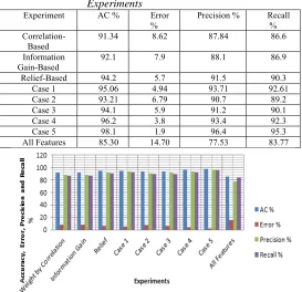
instance which may belong to any of the six topics of online news. The instance may be either popular or unpopular. Table 12 shows the performance metrics for all experiments.
Table 12: Performance Metrics for all Experiments
Experiment AC % Error
%
Precision % Recall %
Correlation-Based
91.34 8.62 87.84 86.6
Information
Gain-Based 92.1 7.9 88.1 86.9
Relief-Based 94.2 5.7 91.5 90.3
Case 1 95.06 4.94 93.71 92.61
Case 2 93.21 6.79 90.7 89.2
Case 3 94.1 5.9 91.2 90.1
Case 4 96.2 3.8 93.4 92.3
Case 5 98.1 1.9 96.4 95.3
All Features 85.30 14.70 77.53 83.77
Figure 18: Performance metrics percentage for all experiments
Table13: Results of the Generated Feature Subset after Applying Logistic Regression
Figure 18 shows the percentage of accuracy, error, precision and recall for the proposed fusion method, the original total number of features in the dataset, and those features produced by the three features selection methods based on correlation, information gain, and Relief. Table 13 shows the results after applying logistic regression using the generated feature subset.
Topics AC % Error % Precision % Recall %
Prediction popular
%
Prediction unpopular
%
Business 95.04 4.9 94.2 94 93 95.5
Entertainment 95.45 4.6 95.5 95.5 95.2 95.5
Lifestyle 95.5 4.5 95.5 95.5 95.5 95.6
Social Media 94.8 6.2 92.4 92.8 92.8 91.8
Technology 95.3 4.7 95.1 95.1 95.1 93.5
[image:10.612.86.303.409.664.2]6979
8. CONCLUSION
This work discussed and investigated the identification of web online news that will be either popular or non-popular. The investigation adopted three different approaches of feature selection. Such approaches are based respectively on correlation, information gain, and relief. The Bayes Network and K-Nearest Neighbor algorithms were adopted and operated for classification and prediction.
This work also proposed a novel method based on selecting and/or fusing the features. There were five different cases of the proposed method. The performance of the proposed method was better than those the three adopted methods. The classification accuracy, recall, and error were improved using that proposed method. The reason for the improvement was due to discarding these irrelevant features which didn't provide class separability. The proposed method manipulated the features that were not considered by the three chosen methods. The manipulation was done depending on two situations. The first one collected those features into groups depending on their semantics and similarity of their natures. The representatives of those groups were taken either the average or the maximum of each group. The second situation was based on selecting only those highly weighted features where their weights are above a predefined threshold. Finally, the performance of the proposed method outperforms all the three adopted ones for the chosen online news dataset. It is also expected that the classification accuracy will be still improved if the proposed method is operated on other datasets.
REFRENCES:
[1] Alexandru Tatar, Marcelo Dias de Amorim, Serge Fdida and Panayotis Antoniadis, “A Survey on Predicting the Popularity of Web Content”, The Journal of Internet Services and Applications, Vol. 5, No. 8, 2014, pp. 1-20.
[2] Kelwin Fernandes, Pedro Vinagre and Paulo Cartez, “A Proactive Intelligent Decision Support System for Predicting the Popularity of Online News, The Proceedings of the 17th Portuguese Conference on Artificial Intelligence, EPIA 2015, Coimbra, Portugal,
September 8-11, 2015, pp 535-546.
[3] Veronica Bolon-Canedo, Naelia Sanchez-Marono and Amparo Alonso-Betanzas, “A Review of Feature Selection Methods on Synthetic Data”, Knowledge and Information Systems, Vol. 34, No. 3, 2013, pp. 483-519.
[4] R. Shreyas, D.M. Akshata, B.S. Mohanad, B. Shagun and C.M Abhishek, “Predicting
Popularity of Online Articles using Random Forest Regression”, The Second International Conference on Cognitive Computing and Informational Processing, Mysore, India, 12-13
Aug. 2016, pp. 1-5, 2016.
[5] He Ren and Quan Yang, “Predicting and Evaluating the Popularity of Online News”, available:
http://cs229.stanford.edu/proj2015/328_report. pdf,
[6] Swati Choudhary, Angkirat Singh Sandhu and Tribikram Pradhan, “Genetic Algorithm Based Correlation Enhanced Prediction of Online News Popularity”, The Proceedings of the International Conference on Computational Intelligence in Data Mining (CIDM), Advances
in Intelligent Systems and Computing, 10-11 December 2016, Vol. 556, pp. 133-144. [7] B. H. Harish and M.B Revanaid dappa, “A
Comprehensive Survey on Various Feature Selection to Categorize Text Documents”, The International Journal of Computer Applications, Vol. 164, No. 8, 2017, pp. 1-7.
[8] S. Dinakaran and P. Ranjit Thangaiah, “Role of Attribute Selection in Classification Algorithms”, The International Journal of Scientific and Engineering Research, Vol. 4,
Issue 6, June 2013, pp. 67-71.
[9] Nadir Elssied, Othnan Ibrahim and Ahmed Osman, “A Novel Feature Selection Based on On-way ANOVA F-test for E-mail Spam Classification”, The Research Journal of Applied Science, Engineering and Technology,
Vol. 7, No. 3, 2014, pp. 625-638.
[10]Danny Roobaret, Grigoris Karakoulas and Nitesh Chawla, “Information Gain, Correlation and Support Vector Machine”, Feature Extraction Foundations and Applications, Studies in Fuzziness and Soft Computing Stud Fuzz, Springer-Verlag Berlin Heidelbery, Vol. 207, 2006, pp. 463-470.
[11]Songtao Shang, Minyong Shi, Wenqian Shang, and Zhiguo Hong, “Improved Feature Weight Algorithm and Its Application to Text
Classification”, Hindawi Publishing
Corporation Mathematical Problems in Engineering, Vol. 2016, pp. 1-12, 2016.
Available:
https://www.hindawi.com/journals/mpe/2016/7 819626/
6980
Information Sciences, Elsevier, Vol. 233, 2013,
pp. 109-125.
[13]M.Akhil Jabbar, B.L Deekshatulua and Priti Chandra, “Classification of Heart Disease Using K-Nearest Neighbor and Genetic Algorithm”,
The International Conference on Computational Intelligence: Modeling
Techniques and Applications (CIMTA),
Kalyani, Kolkata, India, Vol. 10, 2013, pp. 85 – 94.
[14]R.P.L. Durgabai, “Feature Selection using ReliefF Algorithm”, International Journal of Advanced Research in Computer and Communication Engineering, Vol. 3, Issue 10,
October 2014, pp. 8215- 8218.
[15]S. Francisca Rosario, K. Thangadurai, “RELIEF: Feature Selection Approach”,
International Journal of Innovative Research & Development, Vol. 4, Issue 11, October, 2015,
pp. 218-224.
[16]“Pearson’s Correlation Coefficient”, February
17, 2015. Available:
http://www.hep.ph.ic.ac.uk/~hallg/UG_2015/P earsons.pdf
[17]Yongsuo Liu, Qinghua Meng, Rong Chen, Jiansong Wang and Shumin Jiang, and Yuzhu Hu, “A New Method to Evaluate the Similarity of Chromatographic Fingerprints: Weighted Pearson Product–Moment Correlation Coefficient”, The Journal of Chromatographic Science, Vol. 42, No. 1, November 2004, pp:
545–550.
[18]Park HA and Hyeoun-Ae, “An Introduction to Logistic Regression: From Basic Concepts to Interpretation with Particular Attention to Nursing Domain”, Korean Society of Nursing Science, Vol.43, No.2, April 2013, pp. 154-164.
[19]Mark A. Hall and Lloyd A. Smith, “Feature Selection for Machine Learning: Comparing a Correlation-based Filter Approach to the Wrapper”, The Proceedings of the Florida Artificial Intelligence Symposium, FLAIRS-99,
1999. Available:
https://www.aaai.org/Papers/FLAIRS/1999/FL AIRS99-042.pdf
[20]“Predict the Popularity of an Online News
Article”, Available:
https://inclass.kaggle.com/c/predicting-online-news-popularity.
[21]Roja Bandari, Sitaram Asur and Bernardo A. Huberman, “The Pulse of News in Social Media: Forecasting Popularity”, Proceedings of the Sixth International AAAI Conference on
Weblogs and Social Media (In: ICWSM), 2012,
pp. 26-33.
[22]Ramalingam, P. and B. Zheng, “Optimization of a Computer-Aided Detection Scheme using a Logistic Regression Model and Information Gain Feature Selection Method”, Global Journal of Breast Cancer Research, Vol. 1, No.
1, 2013, pp. 1-7.
[23]Thomas W. Miller, “Modeling Techniques in Predictive Analytics”, Business Problems and Solutions with R, Pearson Education, Inc., 2014.
[24]Georgios Rizos, Symeon Papadopoulos and Yiannis Kompatsiaris, “Predicting News Popularity by Mining Online Discussions”, The International World Wide Web Conference
Committee (IW3C2), April 11–15, 2016,
Montréal, Québec, Canada, pp. 737-742. [25]Nuno Moniz, Lu´ıs Torgo and Magdalini
Eirinaki, “Time-Based Ensembles for Prediction of Rare Events In News Streams”, Data Mining Workshops (ICDMW), 2016 IEEE 16th International, Barcelona, Spain, 12-15 Dec. 2016, pp. 1-8.
[26]Prdnya Kumbhar and Manisha Mali, “Survey on Feature Selection techniques and Classification Algorithms for Efficient Text Classification”,
The International Journal of Science and research (IJSR), Vol. 5, Issue 5, May 2016, pp.
1267-1275.
[27]Alper Kursatuysal, “An Improved Global Feature Selection Scheme for Text Classification”, Expert System with Application, ElSEVIER, Vol. 43, 2016, pp. 82-92.
[28]Utthara Gosa Mangai, Suranjana Samanta, Sukhendu Das and Pinaki Roy Chowdhury, “Survey of Decision Fusion and Feature Fusion Strategies for Pattern Classification”, IETE Technical Review, Vol. 27, Issue 4, July-Aug