Basic Paradoxes of Statistical Classical Physics and
Quantum Mechanics
Oleg Kupervasser
Scientific Research Computer Center, Moscow State University, 119992 Moscow, Russia *Corresponding Author: [email protected]
Copyright © 2013 Horizon Research Publishing All rights reserved.
Abstract
Statistical classical mechanics and quantum mechanics are developed and well-known theories that represent a basis for modern physics. Statistical classical mechanics enable the derivation of the properties of large bodies by investigating the movements of small atoms and molecules which comprise these bodies using Newton's classical laws. Quantum mechanics defines the laws of movement of small particles at small atomic distances by considering them as probability waves. The laws of quantum mechanics are described by the Schrödinger equation. The laws of such movements are significantly different from the laws of movement of large bodies, such as planets or stones. The two described theories are well known and have been well studied. As these theories contain numerous paradoxes, many scientists doubt their internal consistencies. However, these paradoxes can be resolved within the framework of the existing physics without the introduction of new laws. To clarify the paper for the inexperienced reader, we include certain necessary basic concepts of statistical physics and quantum mechanics in this paper without the use of formulas. Exact formulas and explanations are included in the Appendices. The text is supplemented by illustrations to enhance the understanding of the paper. The paradoxes underlying thermodynamics and quantum mechanics are also discussed. The approaches to the solutions of these paradoxes are suggested. The first approach is dependent on the influence of the external observer (environment), which disrupts the correlations in the system. The second approach is based on the limits of the self-knowledge of the system for the case in which both the external observer and the environment are included in the considered system. The concepts of observable dynamics, ideal dynamics, and unpredictable dynamics are introduced. The phenomenon of complex (living) systems is contemplated from the point of view of these dynamics.Keywords
Entropy, Schrodinger’s Cat, Observable Dynamics, Ideal Dynamics, Unpredictable Dynamics, Self-Knowledge, And Correlations1. Introduction
A number of important points should be noted.
1) In contrast with other papers regarding paradoxes of quantum mechanics, this paper is not a philosophical paper on physics. We employ scientific methods to consider a solution of these paradoxes. We also construct the physics by excluding these paradoxes and obtain requirements that facilitate their feasibility. The misunderstanding of physics causes these paradoxes and produces physical errors instead of philosophical errors. 2) This paper does not constitute an attempt to provide a new interpretation of quantum mechanics. All interpretations (for example, multi-world interpretation and Copenhagen) aim to provide an evident explanation of quantum mechanics. These interpretations neither solve any paradoxes nor introduce any new appearance in the physics. The author considers all existing reasonable and admissible interpretations. In this paper, a paradox solution is not related to an interpretation but is based on general physics.
3) This paper does notconstitute apopular scientific paper and includes original ideas. The paper is designed for an extensive set of specialists, including biologists, physicists (in quantum mechanics, statistical physics, thermodynamics, and non-linear dynamics), and computer science specialists. Therefore, we have provided a popular review of physics that may be trivial for one expert and useful to another expert. Formulas are not included in this paper; this paper is composed of figures and text. All formulas are contained in the appendices. The author is not a pioneer of this writing style. Examples of this writing style are books by Penrose [1,2], Hofstadter [3], Mensky [4], and Licata [85]. These books are not popular despite their "simplistic" style.
4) This paper includes not only a review of completed papers (although many references are provided) but also includes original ideas of the author.
5) The author does not attempt to discover new laws of physics1. All reviews are conducted within the framework 1 Peierls [7] and Mensky [4] assume that the resolution of the quantum
mechanics measurement paradox is possible by a change in quantum physics laws and the introduction the concept of "consciousness" in physics. Penrose [1, 2] and Leggett [8] assume that the laws of quantum mechanics are broken for substantially large macroscopic systems. However, numerous
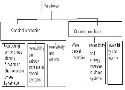
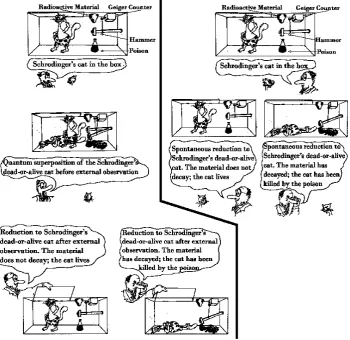
of previously existing physics. The motivation to write this paper was the fact (paradox) that the author has not encountered any paper or physics textbook in which a complete and clear explanation of these paradoxes of physics (Fig. 1) and its consequences is provided. These paradoxes are disregarded in numerous papers, whereas the explanations are incomplete or inaccurate in other papers. In numerous papers, the solution is based on certain interpretations of physics (usually multiworld). New (but not necessary) laws of physics are sometimes used as explanations.
Figure 1 Paradoxes in classical and quantum mechanics
2. Principal Paradoxes of Classical
Statistical Physics
2.1. Macroscopic and Microscopic Parameters of Physical Systems [5, 6]
We begin our discussion from the viewpoint of statistical physics. We examine the gas outflow from a jet engine nozzle (Fig. 2).
[image:2.595.71.288.219.375.2]other physics problems have already been successfully solved without the introduction of new laws. Examples are the Gibbs paradox [9] or the interpretation of spin as a rotation moment of the Dirac electron wave function [10]. Broken symmetries of life or the Universe (such as the symmetry of time direction or the symmetry of right and left) can be explained by a fundamental weak interaction. Weak interaction breaks these symmetries. A complete explanation is included in the Elitzur paper [11]. However, we neglect these small effects and search for other reasons for the asymmetry of time in this paper.
Figure 2 The outflow of gas from a nozzle. Molecules of gas, which are invisible by the naked eye, are magnified.
We observe the distribution of density and velocity of flowing gas for large volumes. These volumes include enormous quantities of invisible molecules. These distinct density and velocity distribution of flowing gas are defined as macroscopic parameters of the system. They provide incomplete descriptions of the system. The complete set of the parameters is includes the velocities and positions of all gas molecules. These parameters are defined as microscopic parameters. Flowing gas is defined as an observable system. The system is considered isolated if it does not interact with its environment. The internal energy of the system is the sum of its molecular energies.
We subsequently consider isolated systems and define internal energy and finite volume (unless the contrary is stated).
2.2. Phase Spaces and Phase Trajectories [5, 6, 12, 17] Here, we introduce the multidimensional space. Coordinates and velocities of all molecules of the system will define the axes of this space. The system will be denoted by a point of this space. The position of this point will provide the complete microscopic description of the system. This space is defined as a system phase space. The system state change, which is featured by the point moving in this space, is defined as a phase trajectory (Fig. 3).
Figure 3 Trajectory in the phase space. A current state of the system described by a point in phase space p, q. The time evolution is described by a trajectory beginning at the initial state point p0, q0.
If we assume that macroscopic parameters are known and microscopic parameters are unknown, the system can be described in phase space by a continuous set of points that correspond to these macroscopic parameters. It is the phase volume ("cloud") of the system or the ensemble of Gibbs (Fig. 4). All points of this volume have equal probability and correspond to different microscopic (but identical macroscopic) parameters. (Appendix A) [5, 6]
[image:2.595.347.517.424.565.2] [image:2.595.75.294.534.681.2]Figure 4. Ensembles in the phase space. The Gibbs ensemble is described by a cloud of points with different initial conditions. The form of the cloud changes during evolution.
For each set of macroscopic parameters (a macroscopic state), the correspondent ensemble of microscopic parameter sets can be obtained. To produce a finite ensemble, we divide the phase space into separate small meshes. This method is defined as discretisation of the continuous space. In this review, the system with a finite volume and a given internal energy can be featured by a major but finite ensemble of states. The corresponding major but finite ensemble of microscopic states can be obtained for each macroscopic state. The properties of the majority of systems are such that a significant part of their possible microscopic states correspond to a principal macroscopic state, which is the equilibrium state. For example, for gas in a given volume, the equilibrium state corresponds to the uniform distribution of molecules in the volume (Appendix E) [5, 6].
2.3. Ergodicity and Mixing [12-14]
The majority of real systems possess the property of ergodicity [13, 14]: almost any phase trajectory should eventually visit all meshes of microstates, which are possible for the given energy of a system. The system should remain for approximately equivalent periods in each microstate mesh. Ergodic systems possess a remarkable property. The average value on time of any macroparametre over a trajectory will be identical for all trajectories. It coincides with the average value over the ensemble of systems featuring thermodynamic equilibrium. This ensemble (referred to as microcanonical) is distributed over a constant energy surface.
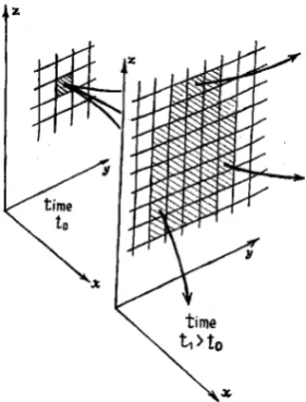
[image:3.595.102.255.81.185.2]The majority of real systems possess a property that is termed chaos or mixing (the first step in describing this property is the so-called KАМ (Kolmogorov-Arnold-Moser) theorem [13, 14], followed by all subsequent theorems). I.e., in the neighbourhood of many points in phase space, there is nearly always another point at which the phase trajectories of these two points diverge exponentially quickly [12- 14] (Figure 5).
Figure 5 Illustration of increased uncertainty increasing or loss of information in a dynamic system. The shaded square at time t0 describes
uncertainty in knowledge of the initial condition.
Indeed, the KAM theorem states that there are persistent portions of phase space in which systems continue to behave like harmonic oscillators. However, the KAM theorem also states that there are noticeable portions of phase space in which harmonic-oscillator systems are destroyed and become chaotic. The KAM theorem describes the mechanism of this destruction. The KAM theorem considers small perturbations of integrable systems. However, for large perturbations (which are applicable for most real systems) and with more degrees of freedom, the portion of the phase space in which the systems continue to behave like harmonic
oscillators becomes small: (http://en.wikipedia.org/wiki/Kolmogorov%E2%80%93Arn
old%E2%80%93Moser_theorem): “The non-resonance and non-degeneracy conditions of the KAM theorem become increasingly difficult to satisfy for systems with more degrees of freedom. As the number of dimensions of the system increases, the volume occupied by the tori decreases. Those KAM tori that are not destroyed by perturbation become invariant Cantor sets, named Cantori by Ian C. Percival in 1979. As the perturbation increases and the smooth curves disintegrate we move from KAM theory to Aubry-Mather theory which requires less stringent hypotheses and works with the Cantor-like sets.”
Pure ergodic or mixing systems are rare (e.g., Sinai’s hard spheres), but the majority of systems are very close to chaotic (ergodic or mixing) systems. For example, weather is predictable only on short time scales because of chaos (the butterfly effect).
Figure 6 Conservation of volume in phase space.
Figure 7 Change in phase volume element in a) stable and b) unstable
cases.
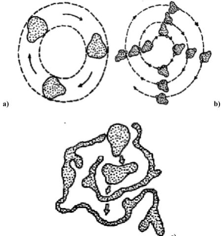
a) b)
c)
Figure 8. Different types of flow in phase space: a) nonergodic flow, b) ergodic flow without mixing, and c) ergodic flow with mixing.
2.4. Reversibility and Poincare's Theorem
Microstate evolution is reversible. For each trajectory in phase space, the inverse trajectory is obtained by the inversion of all velocities of molecules into opposite values. It is equivalent to the reverse demonstration about the process for a film. After a specific duration (most likely large), almost any trajectory returns to its initial microstate. This statement is named Poincare’s theorem (Appendix С) [6]. The majority of real systems are chaotic and unstable, and phase trajectories from previously neighbouring microstates are rapid and divergent. Therefore, the return time for such systems is unequal for previously neighbouring
microstates. It is dependent on the exact position of the initial trajectory point in a mesh that contains a divided phase space. However, for a small class named integrable systems, this return time is approximately identical for all initial points of phase mesh. These returns occur periodically or almost periodically.
2.5. Entropy. [5, 6, 13- 15]
We introduce the basis concept for statistical mechanics—macroscopic entropy. Assume that a certain macroscopic state corresponds to 16 microstates. Using «yes» or «no» answers, how many questions are required to determine which of these 16 microscopic states contains the system? If we consider each microstate, 15 questions are required. A smarter method involves dividing all microscopic states into two groups, with 8 microstates in each group. The first question is to which group does the microstate apply? The specified group will be divided into two subgroups with 4 microstates in each subgroup; we will then ask the same question. We will continue this procedure until a single microstate of the system is obtained. Only four questions, which is the minimal number of questions for the current case, are required. This minimal number of questions can be defined as macroscopic entropy of macrostate [5, 6, 15] (Appendix B). Entropy is simply calculated as the logarithm with basis 2 of the microstate number;the entropy increases with an increase in microstate number. The equilibrium state has maximum entropy as it corresponds to a maximal number of microstates. Entropy is frequently considered a measure of disorder. The greater the disorder in a system, the more questions are necessary to determine the microstate of a system. Therefore, the entropy also increases. Why do we need to introduce an "abstruse" conception as entropy? It would be easier to use the number of microstates instead. However, entropy possesses a remarkable property. We assume that we have a system that consists of two disconnected subsystems. The entropy of a complete system is the sum of two entropies of its subsystems. (The number of questions that correspond to a system is the sum of questions for each of the subsystems). However, the number of microstates are multiplied. Summing the numbers is easier than multiplying the numbers.
Statistical mechanics describes a number of important properties of physical systems:
Let the initial macroscopic state correspond to a certain volume in phase space. A theorem for the reversible Newtonian evolution of the system exists, in which the value of this phase volume is conserved (Appendix F) [6]. Therefore, the number of microstates that correspond to it is also conserved. The entropy that corresponds to this set of microstates is defined as the entropy of ensemble. Based on the conservation of phase volume, the entropy of ensemble is constant over time.
Based on the properties of ergodicity, a system will eventually transfer from almost any initial microstate to an equilibrium state and will remain in this state for the majority of time. During the evolution of a system, the majority of transiting microstates correspond to an equilibrium state. The equilibrium state exhibits maximum macroscopic entropy. If the macroscopic entropy of an initial state was small, it would increase substantially after convergence to thermodynamic equilibrium. This property is opposite of the property of ensemble entropy, which remains constant during evolution. The entropy of ensemble is defined by numerous microstates that do not change during evolution. It is constant and equivalent to the initial number of microstates, whereas macroscopic entropy is defined by a number of microstates that corresponds to a current macroscopic state. Thermodynamic equilibrium involves a large number of microstates.
For chaotic systems (systems with mixing), the following theorem is valid:
Processes of the evolution of macroparametres with macroscopic entropy decreasing are highly unstable with respect to small external noise. In contrast, in the processes of evolution of macroparametres with macroscopic entropy increasing are stable2.
We prove above formulated theorem by considering a process with entropy growth. The initial state of the system is featured by a macroscopic state that is far from thermodynamic equilibrium. This state is characterised with a compact (closed and limited) and convex (containing a straight segment connected by any two points) phase volume. As the system is chaotic, another point is present at an exponentially diverging distance in the neighbourhood of each point. Due to phase volume conservation (Appendix F), another point is always present in the neighbourhood of each phase point, such that these two points exponentially converge and diverge. As a result of mixing, an initially compact phase volume, which is not convex, will completely spread over the constant energy surface in phase. The phase volume possesses a large quantity of "sleeves" or "branches". The full volume of phase "drop" is conserved. "Sleeves" are exponentially expended over their lengths and exponentially shrink over their widths. The number of "sleeves" or "branches" expands; they are incurvate and completely covered by its “net” at the phase energy surface. This process is named as spreading of phase "drop" [13, 14]. Assume that a small external noise has thrown out a phase point from the "sleeve" of a phase drop. However shrinking occurs perpendicularly to the "sleeve," and the phase point moves closer to the "sleeve" and not further from it, which indicates that the process of phase drop spreading is stable with respect to noise.
Therefore, noise can significantly influence a microstate 2 We consider a simple example of ideal gas entropy growth. Gas expands
from a small volume of a box filling this box. The expansion process is distinctly stable with respect to a small amount of noise. Therefore, the inverse process is easily prevented with a small amount of external noise due to the scattering of molecules.
but does not influence a macrostate. A macrostate corresponds to a substantial number of molecular microstates. Although external to each individual molecule, the complete contribution of all molecules to a macrostate remains unchanged. It is related to the “law of large numbers” in probability theory [16]. The majority of microstates, which correspond to a current macrostate, evolve in entropy growth as the probability of this evolution is significant. When the phase drop almost spreads along the entire constant energy surface, its macrostate corresponds to thermodynamic equilibrium. Thus, a small noise cannot distinctly affect its macrostate as the majority of microstates in a system correspond to equilibrium.
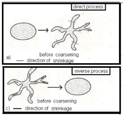
[image:5.595.331.530.429.615.2]We consider an inverse process with decreasing entropy. The initial state is defined by points set in phase space, which are obtained from a direct process («a phase drop» spreading), and the final state is defined by the reversion of molecular velocities. In a reversion of velocities, the initial shape of «a phase drop» does not change. However, the direction of shrinkage due to the reversion of velocities occurs in parallel with its "branches". Shrinkage occurs instead of phase drop spreading. Assume that a small external noise has thrown out a phase point from a "sleeve" of a phase drop. Shrinking occurs in parallel and the spreading occurs perpendicularly to the “sleeve”, which causes the phase point to move away from the "sleeve" instead of approaching it. This condition indicates that the process of phase drop shrinkage is unstable with respect to noise (Fig. 9).
Figure 9. Direct process with an increase in macroscopic entropy and its inverse process. The direction of shrinkage is denoted.
2.7. The Second Law of Thermodynamics and Related Paradoxes
We discuss the second law of thermodynamics and related paradoxes. The second law states the following principles:
thermodynamic equilibrium state [5, 6].
The reversibility is inconsistent with this entropy growth law according to the previously mentioned basic properties of statistical physics.
Due to the reversibility of each process with increasing entropy, an inverse process with decreasing entropy exists. It is paradox of Loschmidt.
Poincare's theorem of returns states that the system must return to an initial state. Its entropy will also return to an initial value. This is a paradox of Poincare.
The concept of the correlations of the velocities and positions of molecules is related to these two paradoxes. 2.8. Additional Unstable Microscopic Correlations and
Their Connection with Paradoxes of Statistical Physics[17])
Correlation is a measure of the mutual dependence of variables. (In our case, it is a measure of the mutual dependence of the velocities and positions of molecules). Pearson’s correlation, which is the most well-known correlation, is a measure of the linear relation of two variables (Appendix D). More complex dependencies and corresponding more complex correlations exist. Correlations between various variables produce restrictions on the possibility of selection of certain values of these variables.
The knowledge of a macroscopic state of a system is a source of correlations. Certain microstates correspond to the given macroscopic state. Thus, their set is already restricted, which will generate to a restriction for possible velocities and positions of molecules, i.e., restriction on the possible microstate of the system. Note that all such correlations are macroscopic and are manifested in dependence between macroscopic parameters of a system. For macroscopic states with small entropy, the restriction on the selection of possible microstates is significant and the quantity of macroscopic parameters and their correlations is also significant. A system at thermodynamic equilibrium entropy reaches the maximum, and the quantity of macroscopic parameters and correlations is small.
Additional or microscopic unstable correlations [17] are defined not only by a knowledge of the current macroscopic state but also by the knowledge of a previous macroscopic history of a system. Assume that the physical system evolved from an initial macroscopic state into another current macroscopic state. Thus, all microscopic states that conform to a current macroscopic state are not possible. Only such states in which the reversion of velocities of molecules produces an initial state can be considered (property of reversibility of motion.): this additional restriction on the states superimposes additional restrictions (correlations) on a set of the microstates that correspond to a current macroscopic state. Additional unstable correlations can be identified in another way; not via knowledge of the past but via knowledge of the future. According to Poincare's theorem, the system should return to a known initial macroscopic initial state after a specific period. By knowing
a certain current macroscopic state and when it will return, we can superimpose additional restrictions (correlation) on a set of microstates that correspond to this current macroscopic state. These correlations are considered unstable as they are extremely unstable with respect to external noise (as will be discussed subsequently). Based on the definition of additional unstable correlations it can be seen that these correlations are close related to Poincare’s and Loschmidt’s paradoxes.
[image:6.595.319.554.395.467.2]These correlations are additional to the macroscopic correlations. (Macroscopic correlations correspond to macrostate representations). The existence of these additional correlations produce a violation of the second law of thermodynamics and ensures a possibility of returns and reversibility, i.e., appearances observed in Poincare’s and Loschmidt’s paradoxes.
Figure 10. Scattering and correlations and correlation flow. Similarly, if the system consists of two non-interacting systems, correlations will only exist inside each system. Returns and reversibility are possible for each of these subsystems. Assume that a small interaction between these subsystems exists. Correlations "will flow" from one subsystem to another, which will create two dependent systems. Only their joint return or reversibility will be possible.
in the system occurs (Fig. 10).
3. Principal Paradoxes of Quantum
Mechanics
3.1. Basic Concepts of Quantum Mechanics—The Wave Function, Schrodinger Equations, Probability Amplitude, Observables, and Indeterminacy Principle of Heisenberg [18, 19]
For clarity, we provide the basic concepts of quantum mechanics.
Motion in quantum mechanics is represented by a wave function and not by a trajectory. Motion is a probability wave; specifically, it is a "probability amplitude" wave, which signifies that the quadrate of the amplitude module of the wave function at some point provides the probability of detecting a particle at this point. The variation in the time of this probability wave is defined by the Schrodinger equation [19]. This is a linear equation, i.e., the sum of its two solutions comprises the solution. Thus, the amplitudes of the probabilities are summed; however, the probabilities are not summed. The probability is defined by the quadrate of amplitude. It imports nonlinearity to the evolution process of a wave function.
Any observable (for example, momentum) is featured by an orthonormal and complete set of functions (a set of eigenfunctions of a observable). The wave function can be expanded to this set of eigenfunctions. Each eigenfunctions set corresponds to a specific value of a observable (eigenvalue). Expansion coefficients provide a probability amplitude for each value. If the wave function is equivalent to an eigenfunction of the observable set, the value of the observable in this case is equivalent to the correspondent eigenvalue. If this is not the case, we can only specify probabilities for various eigenvalues.
The concept of particle velocity has no explicit physical explanation because no well-defined trajectory of a particle exists; only a probability wave exists [19]. Momentum is defined not via a product of velocity and mass but through wave function expansion coefficients over momentum eigenfunctions. This set of eigenfunctions is similar to a complete orthonormal set of Fourier functions used in Fourier analysis.
Coordinate eigenfunctions are proportional to Dirac delta functions. The coefficients of wave function expansion over Dirac delta functions are given by the value of a wave function in an infinite point of a Dirac delta function. The value of a wave function corresponds to the previously defined sense of a wave function as probability amplitudes.
Both momentum and coordinates correspond to various sets of eigenfunctions [19]. Therefore, no wave function, which is in contrast with can simultaneously correspond to both a single momentum eigenvalue and a single coordinate eigenvalue classical mechanics. The explanation for the well-known uncertainty of Heisenberg has been defined [19]
(See Appendix G) and is related to the variation in the definitions of quantum and classical mechanics.
3.2. Pure and Mixed States. Density Matrix [15,18, 20] Quantum mechanics is best described by its wave function, which is the pure state. For classical mechanics, a point in a phase space has similar sense. What is analogous to a classical and statistical ensemble of systems (a cloud of points in a phase space) in quantum mechanics? It is a set of wave functions in which each function corresponds with its probability (instead of the "probability amplitude" for the expansion of a pure state over eigenfunctions). This is the definition of the mixed state.
Assume that a system is part of a larger system. Even if the larger system is represented by a pure state, the smaller subsystem must be generally represented by a mixed state, with the exception of the case in which the pure state of the large system can be described as a product of the small system wave function and its environment wave function. Assume, for example, that the small quantum system interacts with the device that is in a pure state. Although the large system (including the device and the small quantum system) can be represented by a pure state, the small quantum system after measurement is generally already represented by a mixed state.
For equivalent representations of mixed and pure states, the density matrix is used [20]. We select a observable and a corresponding set of eigenfunctions as the density matrix representation based on these eigenfunctions is represented by a square matrix. Every function corresponds to a diagonal element of a density matrix. The value of the element is equivalent to the probability of detecting the corresponding eigenvalue during measurement of the observable.
Nondiagonal elements of a density matrix define the correlations between corresponding pairs of eigenfunctions. Nondiagonal elements possess a maximum value in a pure state; however, their magnitude decreases for the mixed states and can attain a value of zero. The density matrix can always be rewritten over a different set of eigenfunctions that correspond to a different observable. The density matrix provides a maximally complete description of the state of the system. Consequently, the evolution of the density matrix provides a full description of the evolution of the system. (Appendix I.)
3.3. Properties of the Isolated Quantum System with Finite Volume and a Finite Number of Particles [15] Similar to classical systems, we consider the properties of the isolated (closed) quantum system with finite volume and a finite number of particles.
1) These quantum systems evolve for reversible equations of motion (Schrodinger’s equation)
part of all possible classical systems.) Their returns occur in a nearly periodic fashion. The period of these returns is slightly dependent on initial conditions.
3) For quantum systems, it is also possible to define the entropy of ensemble. Entropy is a measure of uncertainty about the state of a system. A pure state provides a maximally complete description of a quantum system. Therefore, any pure state entropy is zero by definition. For the mixed-state case, the system corresponds to a set of pure states. Therefore, entropy already exceeds zero. Assume that the probability of a pure state is near 1. This mixed state is almost pure and its entropy is almost zero. On the other hand, when all pure states of the mixed state have equivalent probabilities, entropy reaches a maximum.
4) During the evolution of a quantum system, the pure state can evolve to a pure state only. In the mixed state, the probabilities of pure states also remain unchanged. Thus, the entropy of ensemble does not change during the evolution of a quantum system.
5) We can represent a large quantum system by a small number of parameters named macroscopic parameters. A large set of pure states defined by microscopic parameters corresponds to this mixed macroscopic state. The entropy of a macroscopic state can be calculated based on this pure set. We define this entropy as macroscopic entropy. In contrast with the entropy of ensemble, the macroscopic entropy should not be conserved during the evolution of a quantum system.
6) A quantum system will not be considered to be an isolated system due to its interaction with the measuring device. Its initial pure state evolves to a mixed state and its microscopic entropy increases. This evolution cannot be reversed by inversion of the measured system as inversion of the measuring device is also necessary.
3.4. Theory of Measurement in Quantum Mechanics [15, 18] (Appendix J, O, P)
To verify a scientific theory, measurements must be performed with measuring devices. A minimum of two measurements are required: a measurements for the initial and a measurements for the final state. If we know the initial state, we can compare the measured final state with the state predicted by theory. Thus, we can verify the accuracy of the theory using this approach.
In classical mechanics, measurement is a simple process of finding current parameters of the system that does not influence its dynamics. In this case, a complete description of the system, which is provided by all microparametres, yields the unique result of measurement.
This situation is substantially much more complicated in quantum mechanics. Measurement influences the dynamics of a quantum system. For a general case of quantum mechanics, we can predict only the probability of a measurement result despite even the full knowledge of its state (The full knowledge of measured system correspond to a pure state).
We explore the measurement process in quantum mechanics. Let the initial system be represented by a wave function. The measurement of some observables causes the situation in which the wave function transfers to an eigenfunction of a observable with a certain probability. This eigenfunction corresponds to a measured value of a observable, which is equivalent to its eigenvalue. As previously stated, the probability of this measurements is proportional to the quadrate of the amplitude of the wave function. The probability is obtained by expansion to eigenfunctions. After measurement , the system transfers from a pure state to a mixed state and is an ensemble of these possible measurement results with corresponding probabilities. This process is named the reduction of wave function. It is not described by Schrodinger’s equation. The Schrodinger equation describes the evolution from a pure state in the pure one. The result of a reduction is a mixed state obtained from an initial pure state. The Schrodinger equation is reversible. The process of reduction is nonreversible. The second type of quantum evolution is possible as the quantum system is not isolated during measurement —it interacts with the macroscopic classical device.
To be consistently represented by quantum mechanics, the macroscopic device should be ideally macroscopic, i.e., either to exist in infinite space or to consist of an infinite number of particles. The ideal macroscopic device does not obey Poincare's theorem of returns and exhibits a certain macroscopic state during all moments of measurement. For the ideal macroscopic device, quantum laws yield the same results as classical laws during any finite period. Note that the real measuring device (i.e., in a finite volume with a finite number of particles) is approximately macroscopic. This condition is essential to our future analysis as it is the main source of the paradoxes considered in the subsequent section. Thus, the evolution of a quantum system is divided into two aspects. The first aspect is reversible—Schrodinger’s evolution. The second aspect is the nonreversible reduction of the wave function, which occurs at the interaction with the macroscopic classical device.
“mysteriousness” does not exist.
3.5. Complexity of an Attempt of a "Classical"
Interpretation of Quantum Mechanics: Introduction of Hidden Parameters and Paradox EPR [18, 103] The laws of quantum mechanics are probabilistic, and many observables cannot be measured simultaneously. However, many laws of classical statistical mechanics are also probabilistic. Their probabilistic nature can be attributed to hidden microscopic parameters (Appendix U): the velocities and positions of all molecules. Any classical macroscopic state is featured by a set of possible corresponding microstates. Similarly, we can try to interpret a quantum probability by introducing hidden parameters. The knowledge of these hidden parameters enables the unique determination of all variables in the quantum system. Similarly, regarding the macroscopic classical state, an observed state in quantum mechanics corresponds to a set of possible values for the hidden parameters. However, the existence of these hidden parameters is possible in quantum mechanics only under the following assumptions:
1) Measurement (with the exception of special cases in which one of the observable eigenfunctions is equivalent to the wave function of the observed system) changes the state of the observed system. In a classical case, it is possible (at least in principle) to perform any measurement without the perturbation of the observed system.
2) All hidden parameters cannot be measured simultaneously. Note the Heisenberg uncertainty principle. The measurement changes a system state (a wave function reduction) and thus all hidden parameters cannot also be measured by a set of sequential measurements. All hidden parameters possess well-defined values. However, there is no such real and observable physical state in which all hidden parameters possess these well-defined values; a probability distribution exists. In any real experiment, we can measure only a part of these parameters. This measurement will simultaneously produce uncontrollable perturbation for the remainder of the parameters.
3) Existence of the hidden parameters in quantum theory is impossible without introduction of long-range interactions [18]. This long-range interaction acts instantaneously across an infinite distance. However, there is no contradiction with the relativity theory maximal velocity limit as this interaction cannot transfer any information or mass. As the parameters
are hidden; the interaction between them is also hidden and not observed. The observed appearances can be explained by the correlation of random values.
This necessity of introduction of unobserved long-range interaction is a high price for classical "presentation". The interpretation of hidden parameters is not used in the literature about quantum mechanics. It is easier to consider the laws of quantum mechanics as a mathematical method for the calculation of typical random correlations of observable macroscopic parameters for measuring devices.
This necessity of introduction of long-range interactions of the hidden parameters is illustrated by the well-known Einstein-Podolsky-Rozen "Paradox" (EPR) [18] (Appendix R). This "paradox" is fictitious and is derived from a classical interpretation (i.e., interpretation of hidden parameter) of quantum mechanics by the use of "the small price" (i.e. without long-range interaction).
This paradox is based on an analysis of electron-positron pair states. Initially three particles were in proximity; they subsequently scattered over a large distance.
Figure 11. EPR experiment
Assume that spin projections have "classical" interpretations as hidden parameters. Measurement yields previously hidden values. Why does the dependence of measured spin projections of an electron and a positron exist? Are these common random correlations? Does a long-distance interaction between the hidden parameters exist? Using Bell’s inequality (Appendix T), it is possible to prove the following theorem: There is no set of hidden parameters such that the probability distributions of these hidden parameters can explain the mutual probabilities calculated from quantum mechanics without introducing a long-distance interaction between these hidden parameters. The interaction of long-distance spins must exist in hidden spins theory.
However, it is possible to not consider all of the hidden parameters but only the results of measurement. In this case, the dependence between the electron and positron spins can be easily explained using typical random correlations between the measured parameters. We can simultaneously measure only two projections of a spin (one projection for an electron and one projection for a proton) from numerous possible hidden parameters.
The dependence between long-range objects is defined as a quantum correlation. This correlation cannot be explained by hidden parameters without the long-range interaction of these hidden parameters. This explanation is always possible for classical correlations. After measurement, the quantum correlations are transformed to classical correlations.
The introduction of hidden parameters in quantum mechanics is impossible without long-range interactions between these parameters. It is possible to disregard hidden parameters and to consider quantum mechanics, such as a mathematical apparatus provides random dependence between the measured properties of large classical devices. In this case, long-range interaction is not required. Dependence between observed values can be explained by random correlation. Correlation exists as the measured quantum objects initially co-existed.
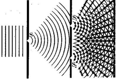
3.6. Problem of Two Slots As an Illustration of the Complexity of Quantum Mechanics [96,97,104]
Due to the impossibility of an "easy" classical interpretation of quantum mechanics, a well-known American physicist named Richard Feynman assumed that nobody understands quantum mechanics. He noted that «the single secret of quantum mechanics can be expressed by just one experiment using a double slot and electrons. It is a modified version of a simple classical experience in 1801 by an English scientist Thomas Young, who demonstrated the wave nature of light. In Young’s experiment, light from a source (a narrow slot S) illuminates a screen with two closely positioned slots S1 and S2. While transiting through each of the slots, the light is scattered by diffraction; therefore, the light beams that have transited through slots S1 and S2, were overlapped on a white screen E. In the field of overlapping light beams, numerous alternating light and dark bands formed—we define this overlapping as an interference pattern. Young interpreted the dark lines as places in which "crests" of light waves from one slot meet "troughs" of waves from the other slot and quench each other. The bright lines occur in places in which crests or troughs from both slots coincide, which amplified the light. During almost two hundred years, variants of the two-slot-hole Young experiments were considered to be proof of the nature of waves on water, radio signals, X-rays, sound and thermal radiation (Fig. 12).
Figure 12. Young’s experiment with light.
[image:10.595.331.527.581.714.2]difference in the distances from the two slots to this point, which is measured in wave length units, is named the path difference for this point. If it is an integer, the maximum wave occurs at this point. If it is an integer and a half, the minimum occurs at this point.
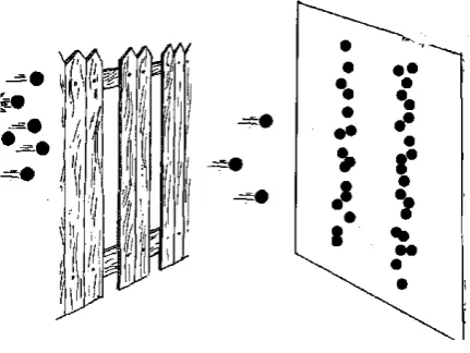
It is remarkable that Young’s experiment can also be conducted with electrons (Fig. 13,14). Instead of a sunlight beam, a beam of electrons transits through parallel slots. The screen plate is coated with a luminophor (similar to the screen of a television tube). Each electron colliding with the luminophor produces an illuminating point, which registers its arrival in the form of a common particle. However, the image generated by all electrons yields a surprising impression. The image gives an interference pattern similar to the pattern obtained in the case of light. The image contrasts with the pattern that we would obtain by throwing balls at a fence with two boards removed (similar to two slots). The two-slot-hole experiment with electrons demonstrates that these particles can behave as a wave.
[image:11.595.77.282.310.422.2]Figure 13. Young’s experiment with electrons.
Figure 14. Young’s experiment with balls and a fence.
If one of the slots is closed in the two-slot electron diffraction experiment, an interference pattern disappears. Instead, the band of the electrons is registered. We open the second slot and close the first slot. In this manner, we obtain the second band. The final pattern is similar to the pattern obtained by the ball game described previously, i.e., a simple sum of these two bands. However, if both slots are opened simultaneously, we observe a complex interference pattern. The results of this experiment cannot be explained by the interaction of electrons—the same result is obtained by
emitting electrons one at a time—as an electron position is not defined by a specific trajectory but by a wave of probabilities. The two waves from the two slots are summed to yield an interference pattern. The quadrate of the amplitude of sum of these two waves on the screen yields the probability of locating an electron in this area.
Assume that we arrange a detector that shows the slots through which an electron transits. In this case, the final pattern is similar to the results of the experiment with alternately closed slots, i.е., the interference pattern disappears. This result is explained by the influence of the measuring device—the detector. A reduction of wave function occurs, and it’s pure state transfers to the mixed state. Thus, instead of the sum of wave amplitudes from two slots, the probabilities are condensed and the interference pattern disappears.
This experiment demonstrates two main properties of quantum mechanics. First, we cannot predict the exact final position of an electron on the screen but we can discover the probabilities of all points. Only a large number of electrons produces a certain and predictable distribution pattern on the screen. In the classical case, the result was predictable for a single particle. Second, we cannot perform any measurement of the intermediate state of an electron without perturbation of this intermediate state that causes variation in the measurement results. After observing which slots the electron has transited, we destroy the additional interference pattern. In classical mechanics, it is always possible, at least in principle, to perform a measurement without the perturbation of the system dynamics. In quantum mechanics, this measurement is possible only if the wave function of the measured system is identical to an eigenfunction of an observable.
The experiment with two slots also facilitates an explanation of the mechanism of the vanishing of quantum interference effects for macroscopic systems, which occurs under the following three requirements:
1) A coherent "monochromatic" wave, which is considered in the experiment, interacts with its environment or its source. This interaction causes the transformation of its pure state to the mixed state. Consequently, the probability wave does not consist of an infinite sine curve but of a set of sine curve segments. This segment of the sine curve is named a wave packet. A phase of a wave packet possesses a random value. The length of a wave packet is approximately 10–20 wave lengths with the order of wave-atom interaction radius. The atoms correspond to the surrounding medium or the source. 2) Consider a system with a macroscopic size. The distances between the slots (D) are significantly larger than the lengths of a wave packet (n λ) and the distances from the slots to the screen (L). Precisely, D>> (L∙nλ)1/2, where λ is a wave length.
[image:11.595.72.288.453.615.2]As the distance between slots increases (at constant value L), the path difference becomes much larger than the length of a wave packet for the majority of points on the screen. As result, the phases of the waves that originate at the slots become random. Thus, coarsened macroscopic intensities are condensed rather than the amplitudes of the waves. The interference disappears for the majority of points on the screen. As the distance between the slots becomes larger than the distance to the screen, the interference remains in the small neighbourhood of a screen point, which would be precisely between the slots. The size of an interference range becomes equivalent to a wave packet. As the distances between slots increase, the wave intensity in this interference range begins to decrease and converges to zero without a decrease in size3. Thus, small interference effects are not observed for coarsened (i.e., macroscopic) descriptions.
These effects of loss of interference are caused by the macroscopic nature of the system and its parameters and by the mixed nature of the initial state. This transformation of a wave from a pure coherent state to a mixed state due to interaction (entangling) with its environment is named decoherence (from the Latin cohaerentio—connection) [21-25] (Appendix P). The system is mixed or entangled with a surrounding medium. For macroscopic (i.e., very large) systems, decoherence causes a loss of quantum interference, as discussed previously in the experiments with two slots. The decoherence theory has an important consequence: for macrostate quantum theory, the predictions almost coincide with the predictions of classical theory. However, the price for this coincidence is irreversibility, as will be subsequently discussed.
3.7. Schrodinger’s Cat Paradox [26] and Spontaneous Reduction [18, 98]
The complete violation of the wave superposition principle (i.e., the complete vanishing of interference) and the wave function reduction occurs only during the interaction of a quantum system with an ideal macroscopic object or device. The ideal macroscopic object either possesses infinite volume or consists of an infinite number of particles. Such an ideal macroscopic object can be consistently described by quantum and classical mechanics4.
We consider (unless the other is assumed) only systems with finite volume with a finite number of particles, which is
3 Note that this system has an infinite size in the wave propagation direction
and the screen with interference (its distance to the screen with slots is constant and equal to L) does not reflect the wave. Therefore, in contrast with the finite systems considered in the subsequent section, the interference does not reappear after it disappears. Conversely, when the distance between the slots converges to infinity (at the constant value L), the effects of quantum interference converge to zero (for any finite wave packet length and for any finite degree of macroparameter coarsening).
4 Thus, by observing the light of a remote star, we study the light but do not
influence the light as the observation may have been expected on the basis of quantum measurement theory. We only change the state of star photons that reach us as we consider the Universe space as infinite. Thus, illuminated photons have no chance of returning to a star and changing its state. In the case of the finite Universe, observable photons can return to a star and influence it. However, for an extremely large Universe, an extremely long period may be required.
similar to the classical case. Such devices or objects can be considered as only approximately macroscopic5.
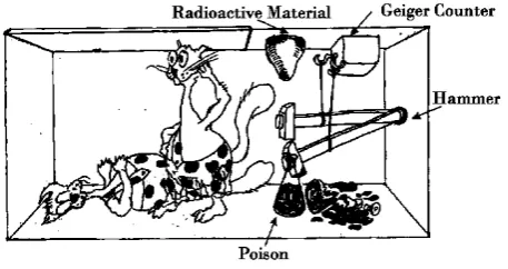
A real experiment demonstrates that, for nonideal macroscopic objects, the destruction of superposition and corresponding wave function reduction may occur. We define this reduction of imperfect macroscopic objects as spontaneous reduction. Despite its tremendous successes, spontaneous reduction produces paradoxes that produce doubt in the completeness of quantum mechanics. We reduce the most impressive paradox from this series— Schrodinger’s cat paradox (Schrodinger 1935) [26] (Fig. 15).
Figure 15. Experiment with Schrodinger’ cat.
Schrodinger’s cat paradox is a thought experiment that clarifies the principles of superposition and wave function reductions. A cat is placed in a box. With the exception of the cat, there is a capsule with poisonous gas (or a bomb) in the box, which can detonate with a 50 percent probability due to the radioactive decay of a plutonium atom or a casually illuminated light quantum. After awhile, the box is opened and it is revealed whether the cat is still alive. Until the box is opened (measurement is not performed), the cat stays in a strange superposition of two states: "alive" and "dead". For macroobjects, this situation appears to be mysterious6. (Therefore, for quantum particles, the superposition of two different states is natural.) No basic prohibition for the quantum superposition of macrostates exists.
The reduction of these states by an external observer at the moment the box is opened does not produce any inconsistency in quantum mechanics. It is easily explained by the interaction of the external observer with the cat during the evaluation of the cat’s state.
However, the paradox arises in the closed box when the observer is the cat. The cat possesses consciousness and is capable of observing both itself and the environment. After introspection, the cat cannot be simultaneously alive and dead but must exist in one of these two states. Experience demonstrates that any conscious creature feels alive, otherwise it is dead. These situations do not exist simultaneously. Therefore, spontaneous reduction to two possible states (alive and dead) occurs7. The cat, along with 5 For example, this star-observer system in a large finite Universe would
behave similarly to an infinite Universe only during a long finite period.
6 These situations can be described with art, such as the use of using
"paradoxical" images [3, 28], (Appendix V).
7 Certain attempts have been made to understand how the consciousness can
perceive these exotic states of macro-objects [3, 28], (Appendix V, and the
[image:12.595.320.549.218.339.2]
the contents of the box, does not represent an ideal macroscopic object. Thus, an observable and nonreversible spontaneous reduction contradicts reversible Schrodinger quantum dynamics. In this case, it cannot be explained by an external influence, as the system is isolated. [18, 27, 7].
Numerous problems are related to spontaneous reduction. Does spontaneous reduction actually contradict Schrodinger quantum dynamics? When the system is substantially macroscopic, does spontaneous reduction occur? Must a macroscopic system have a consciousness similar to the consciousness of the cat? When does spontaneous reduction occur?
3.8. Zeno Paradox or the Paradox of a Kettle that Never Boils
The "the paradox of a kettle that never boils" is related to the last previously mentioned problem. Two paradoxes are discussed.
Assume a quantum process. For example, the decay of a particle or transmission of a particle from one energy level to another level.
The first paradox is as follows: If intervals between acts of registering converge to zero, then the specified process never occurs during any chosen finite interval. This paradox can be explained by the influence of quantum measurement. Measurement causes a reduction to the mixed state (broken and unbroken particles). The relative process rate (over one particle) converges to zero when the measurement interval converges to zero. These two facts cause an end to the process of frequent measurements.
The second paradox is as follows: In real life, the decay of a substance that contains numerous particles is always represented by exponential law. The decay is not casual. The relative velocity of this decay is constant over time. It is impossible to determine the observational "age" of this substance if we do not know the initial quantity of unbroken particles and the quantity of particles that are removed from the system. However, quantum decay, according to the quantum mechanical equations, is not described by exponential law. Therefore, the relative rate of decay is zero at the beginning of the process and, subsequently, increases. We paradoxically conclude that it is possible to introduce a nonphysical concept of the system—"age". "Age" can be easily determined through the current relative rate of system decay.
We will resolve this second paradox in the part of the paper concerned with observable dynamics.
3.9. Quantum Correlations of System States and their Connection with the Paradox of Schrodinger’s Cat The concept of the quantum correlation of system statesis closely related to the paradox of Schrodinger’s cat. Assume a spontaneous reduction of states of the living or dead cat. Any
previous references).
additional measurement will be dependent on the previous state of the cat. The cat is either "living" or "dead". The observed data can be divided into two nonoverlapping groups: one group corresponds to a “living cat” and the other group corresponds to a "dead cat". However, if the cat is in a quantum superposition of these two states, the results of the additional measurements will be dependent on both states of the cat. It cannot be divided into two nonoverlapping groups. This connection between initial states, for which the division of additional results of measurement into independent nonoverlapping groups corresponds to these initial states, is named the "quantum correlation of system states".
In mathematical language, this fact is explained by the nonlinearity of the connection between the probability of observed data and a wave function. The quadrate of the sum is not equivalent to the sum of the quadrates. Additional terms (or the interference terms) are the measures of quantum correlations.
Quantum correlations also correspond to nondiagonal elements of a density matrix. For the mixed state obtained from measurement, all nondiagonal terms are zero.
We express the paradox of Schrodinger’s cat in the language of quantum correlations. Introspection about the cat provides only one of two possible results: a "living cat" or a "dead cat". Thus, spontaneous reduction exists, and a quantum correlation between these states disappears, which indicates that additional results of measurement can be divided into two independent nonoverlapping groups that correspond to the initial states.
According to Schrodinger’s equations, a quantum correlation cannot disappear by itself without the presence of external forces. Additional measurement results cannot be divided into two independent nonoverlapping groups that correspond to the initial states.
This inconsistency between Schrodinger dynamics and the observable spontaneous reduction produces the paradox.
4. Quantum Mechanics Interpretations:
Their Failure to Solve Paradoxes
One of the problems that we discussed previously is the difficulty of understanding quantum mechanics based on our classical intuition of real word experience. Various interpretations of quantum mechanics, which [18] can facilitate this understanding, exist. Note that none of the interpretations of quantum mechanics can solve the previously mentioned paradoxes; they only enable a visual, distinct and intuitive understanding of quantum mechanics. From an extensive list of possible interpretations, we restrict this discussion to three interpretations. The multiworld interpretation is currently the most popular interpretation.
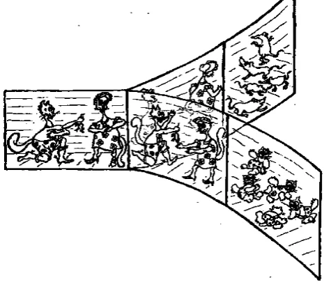
4.1. Multiworld Interpretation. [29, 30, 18, 99]
quantum evolution can generate various and macroscopically distinguishable conditions. We observe only one of these conditions. A multiworld interpretation states that although these states simultaneously exist in certain “parallel worlds”, we (or a cat in our mental experiment) can only observe one macroscopic alternative.
Figure 16. Multiworld interpretation.
A similar approach illustrates the concept of spontaneous reduction: As all worlds exist simultaneously, they all have the capability of influencing measurement results. Generally, measurement results cannot be divided into two disconnected groups related to the living and dead cat. This observation signifies that these worlds are correlated and each influences the measurement results. The presence of spontaneous reduction in measurement causes a loss of this correlation. The measurement results separate into independent groups that correspond to various worlds (Fig. 16).
The multiworld interpretation does not explain the paradox of Schrodinger’s cat. The cat observes only one of the existing worlds. The results of additional measurements are dependent on correlations that exist between the worlds. However, neither these worlds nor these correlations are observed. «Parallel worlds» that we know nothing about can exist. These worlds can significantly affect the results of
future experiments, i.e., knowledge of only the current state (in our "world") and the laws of quantum mechanics does not enable us to probabilistically predict the future. However, quantum mechanics have been developed for these predictions. Nevertheless, based on a spontaneous reduction, which destroys the quantum correlations between the worlds, we can predict the future using knowledge of only the current (and observed) state of our "world". We see that the paradox of Schrodinger’s cat returns, but in a different form.
The multiworld interpretation does not solve some problems. For example, the definition of macroscopic states that correspond to “separation” of “the parallel worlds” is unclear. (The wave function expansion is ambiguous, and different sets of orthogonal functions can be employed for this purpose.) The approach for obtaining the exact moments of time when this "separation" occurs is unclear. However, obtaining solutions for the paradoxes (in contrast with a common error) is not the purpose of interpreting quantum mechanics.
4.2. Copenhagen Interpretation [100]
The Copenhagen interpretation, which has been referenced in existing studies, is a standard for the majority of books and papers in the field of quantum mechanics. It states that at the moment of the observation of macroscopic states, spontaneous reduction occurs and quantum correlations disappear. Thus, the paradoxes described previously are generated.
Note that the reduction in the Copenhagen interpretation occurs only for a chosen final observer in the sequence of measurements. The reduction can be different for different observers. Indeed, the experiment should be described from the observer’s point of view. The reduction, similar to the velocity of the system, is dependent on the choice of the observation system.
[image:14.595.59.292.154.360.2]Figure 17. Schrodinger’s cat experiment from the viewpoint of an external observer (the experimenter) and from self-observation (the cat)
From the point of view of an external observer, the reduction occurs when the external experimenter opens the box and interacts with the cat, which results in the reduction. No paradox exists for the external observer.
Only when the cat is regarded as the final observer does spontaneous reduction occur and, consequently, the paradox described previously exists. The cat can only feel alive or be dead but cannot simultaneously exist in these two states.
This observation is very important as its misunderstanding can produce erroneous statements [29, 30], such as the Copenhagen interpretation, which is incompatible with the multiworld interpretation. The difference between these interpretations are not observable; thus, both interpretations can be employed.
4.3. Interpretation Via Hidden Parameters. [18], (Appendix S,T,U)
Introduction of the hidden parameters defines another interpretation related to the EPR paradox, such as the wave-pilot theory of de Broglie-Bohm [18]. This theory includes coordinates, velocities, spins and wave functions (wave- pilot) that change over time, according to Schrodinger equations, as hidden parameters. Thus, quantum correlations (as presented during the discussion of the EPR paradox) produce a locality violation, i.e., long-range
interactions among the hidden parameters. For an explanation of the connection among actual measured (not hidden) parameters, such long-range interactions are not necessary. These connections are perfectly described by the typical correlations of variables. Thus, the reduction of a macroscopic state (or a state that occurs at measurement or that is spontaneous) causes the quantum correlations, which become classical correlations, to vanish.
The difference between quantum correlations and classical correlations, which occur after reduction, is expressed not only by existing long-range interactions. Let the correlated long-distance parts of the system (these parts that initially existed in a pure state) appear together after a considerable period of time. Thus, in a quantum case, we again obtain a pure state, but in the classical case, reduction (or a reduction that occurs at measurement or that is spontaneous)—the mixed reduction—also occurs. Spontaneous reduction creates inconsistency in the Schrodinger evolution. Paradoxes do not disappear but only acquire different appearances.
observer and a surrounding medium in a complete system because, in many cases, even their small influence cannot be neglected. As will be subsequently explained, this necessity of taking into account of the observer’s influence is valid not only for quantum mechanics but also for classical mechanics. Generally, a complete system consists of three parts: the observable system, the surrounding medium, and the observer. The observer also consists of three parts: the measuring device, the observer and the memory of the observer. Memory is required for maintaining the sequence of observation. This observation sequence can be employed for the comparison with the theory. Memory must be isolated from its entire environment, with the exception of the channel of receiving information. If certain external factors can influence, change or delete its contents, no experiments for theory verification are possible. This statement, which is critical, helps to resolve many paradoxes, including the paradoxes considered in the subsequent section.
The final point of the complete physical system is the observer's memory. The system includes only one observer. Although many observers can exist, we choose the point of view of only one observer. The remaining observers are considered as parts of the observable system or the environment. Which observer must be chosen? The problem is solved using an approach that is similar to relativity theory—it is possible that any observer can be selected. However, it is important to interpret all facts from the point of view of the single chosen observer. For the case of Schrodinger’s cat paradox, the observer can be either the cat or the external observer (but not both).
6. Solution of the Paradox of
Schrodinger’s Cat
Note, the paradox of Schrodinger’s cat is inconsistent with regards to the spontaneous reduction observed by a cat and the evolution by Schrodinger forbidding such a reduction. To understand the paradox of Schrodinger’s cat, it is necessary to consider the paradox from the point of view of two observers: the external observer and the cat, i.e., introspection.
In the case of the external observer-experimenter, the paradox does not occur. If the experimenter attempts to determine whether the cat is alive, it inevitably influences the observable system (in agreement with quantum mechanics), which causes a reduction. The system is not isolated and thus cannot be represented by a Schrodinger equation. The reducing role of the observer can also be played by the surrounding medium. This case is defined as decoherence. In this case, the role of the observer is more natural and reduced to fixing decoherence. In both cases, the measured system is entangled with the environment or the observer, i.e., correlations of the measured system exist with the environment or the observer.
What will occur if we consider the closed complete physical system, including the observer, observed system
and environment? This is the case of the cat introspection. The system includes the cat and his box environment. Note that complete introspection (complete in the sense of quantum mechanics) and the complete verification of the laws of quantum mechanics is impossible in the isolated system, including by the observer. We can precisely measure and analyse a state of an external system in principal. However, if we also include ourselves in the consideration, natural restrictions exist. This occurrence is related to the possibility of retaining memory and the analysis of the states of molecules using these molecules. This assumption produces inconsistencies (Appendix M). Therefore, the possibility of experimentally establishing the inconsistency between Schrodinger evolution and spontaneous reduction using introspection in an isolate system is also restricted.
We discovered mental experiments that cause inconsistency between Schrodinger evolution and spontaneous reduction.
1) The first example is related to the reversibility of quantum evolution. Assume that we have introduced a Hamiltonian that is capable of reversing the quantum evolution of the cat-box system [29, 30]. Although it is almost practically impossible, no theoretical impossibility exists. If spontaneous reduction occurs, the process would be nonreversible. If spontaneous reduction does not occur, the cat-box systemwill return to an initially pure state. However, only the external observer can construct such a validation. The cat cannot validate this observation through introspection because the cat’s memory will be erased after returning to an initial state.
No paradox exists from the point of view of the external observer as he does not observe a spontaneous reduction that can produce a paradox.
2) The second example is related to the necessity of Poincare's return of a quantum system to an initial state. Assume that the initial state was pure. If a spontaneous reduction exists in the case of cat introspection, the reduction produces a mixed state. Return would be impossible—the mixed state cannot transfer to a pure state according to Schrodinger equations. Thus, if the cat has a fixed return, it would result in an inconsistency with spontaneous reduction. However, the cat cannot achieve a fixed return (in the case of the fidelity of quantum mechanics) because a return will erase the cat's memory. Therefore, no paradox exists.
The external observer can observe this return by measurement of the initial and final state of this system. No paradox exists as the observer does not observe a spontaneous reduction that can generate a paradox (Fig. 18).