September 5, 2017
Precise masses for the transiting planetary system HD 106315 with
HARPS
?
S. C. C. Barros
1??, H. Gosselin
2,23, J. Lillo-Box
3, D. Bayliss
4, E. Delgado Mena
1, B. Brugger
2, A. Santerne
2,
D. J. Armstrong
5, V. Adibekyan
1, J. D. Armstrong
6, D. Barrado
7, J. Bento
8, I. Boisse
2, A. S. Bonomo
9, F. Bouchy
4,
D. J. A. Brown
5, W. D. Cochran
10, A. Collier Cameron
11, M. Deleuil
2, O. Demangeon
1, R. F. Díaz
4,12,13, A. Doyle
5,
X. Dumusque
4, D. Ehrenreich
4, N. Espinoza
14,15, F. Faedi
5, J. P. Faria
1,16, P. Figueira
1, E. Foxell
5, G. Hébrard
17,18,
S. Hojjatpanah
1,16, J. Jackman
5, M. Lendl
19, R. Ligi
2, C. Lovis
4, C. Melo
3, O. Mousis
2, J. J. Neal
1,16, H. P. Osborn
5,
D. Pollacco
5, N. C. Santos
1,16, R. Sefako
20, A. Shporer
21, S. G. Sousa
1, A. H. M. J. Triaud
22, S. Udry
4, A. Vigan
2, and
A. Wyttenbach
41 Instituto de Astrofísica e Ciências do Espaço, Universidade do Porto, CAUP, Rua das Estrelas, PT4150-762 Porto, Portugal e-mail:
2 Aix Marseille Univ, CNRS, LAM, Laboratoire d’Astrophysique de Marseille, Marseille, France
3 European Southern Observatory (ESO), Alonso de Cordova 3107, Vitacura, Casilla 19001, Santiago de Chile, Chile 4 Observatoire Astronomique de l’Universite de Geneve, 51 Chemin des Maillettes, 1290 Versoix, Switzerland 5 Department of Physics, University of Warwick, Gibbet Hill Road, Coventry, CV4 7AL, UK
6 Institute for Astronomy, University of Hawaii, 34 Ohia Ku Street, Pukalani, Maui, Hawaii 96790
7 Depto. de Astrofísica, Centro de Astrobiología (CSIC-INTA), ESAC campus 28692 Villanueva de la Cañada (Madrid), Spain 8 Research School of Astronomy and Astrophysics, Australian National University, Mount Stromlo Observatory, Cotter Road,
Weston Creek, ACT 2611, Australia
9 INAF – Osservatorio Astrofisico di Torino, Strada Osservatorio 20, I-10025, Pino Torinese (TO), Italy 10 McDonald Observatory and Department of Astronomy, The University of Texas at Austin, Austin Texas USA
11 Centre for Exoplanet Science, SUPA School of Physics & Astronomy, University of St Andrews, North Haugh ST ANDREWS,
Fife, KY16 9SS
12 Universidad de Buenos Aires, Facultad de Ciencias Exactas y Naturales. Buenos Aires, Argentina
13 CONICET - Universidad de Buenos Aires. Instituto de Astronomía y Física del Espacio (IAFE). Buenos Aires, Argentina. 14 Instituto de Astrofisica, Facultad de Fisica, Pontificia Universidad Catolica de Chile, Av. Vicuna Mackenna 4860, 782-0436 Macul,
Santiago, Chile
15 Millennium Institute of Astrophysics, Av. Vicuna Mackenna 4860, 782-0436 Macul, Santiago, Chile
16 Departamento de Fisica e Astronomia, Faculdade de Ciencias, Universidade do Porto, Rua Campo Alegre, 4169-007 Porto, Portugal
17 Institut d’Astrophysique de Paris, UMR7095 CNRS, Universite Pierre & Marie Curie, 98bis boulevard Arago, 75014 Paris, France 18 Aix Marseille Univ, CNRS, OHP, Observatoire de Haute Provence, Saint Michel l’Observatoire, France
19 Space Research Institute, Austrian Academy of Sciences, Schmiedlstr. 6, 8042, Graz, Austria 20 South African Astronomical Observatory, PO Box 9, Observatory, 7935
21 Division of Geological and Planetary Sciences, California Institute of Technology, Pasadena, CA 91125, USA 22 Institute of Astronomy, University of Cambridge, Madingley Road, CB3 0HA, Cambridge, United Kingdom 23 Université de Toulouse, UPS-OMP, IRAP, Toulouse, France
Received ??, ??; accepted ??
ABSTRACT
Context.The multi-planetary system HD 106315 was recently found in K2 data . The planets have periods ofPb ∼9.55 andPc ∼
21.06 days, and radii ofrb=2.44±0.17R⊕andrc=4.35±0.23R⊕. The brightness of the host star (V=9.0 mag) makes it an excellent
target for transmission spectroscopy. However, to interpret transmission spectra it is crucial to measure the planetary masses.
Aims.We obtained high precision radial velocities for HD 106315 to determine the mass of the two transiting planets discovered with Kepler K2. Our successful observation strategy was carefully tailored to mitigate the effect of stellar variability.
Methods.We modelled the new radial velocity data together with the K2 transit photometry and a new ground-based partial transit of HD 106315c to derive system parameters.
Results.We estimate the mass of HD 106315b to be 12.6±3.2M⊕and the density to be 4.7±1.7g cm−3, while for HD 106315c we
estimate a mass of 15.2±3.7M⊕and a density of 1.01±0.29 g cm−3. Hence, despite planet c having a radius almost twice as large as
planet b, their masses are consistent with one another.
Conclusions.We conclude that HD 106315c has a thick hydrogen-helium gaseous envelope. A detailed investigation of HD 106315b using a planetary interior model constrains the core mass fraction to be 5-29%, and the water mass fraction to be 10-50%. An alterna-tive, not considered by our model, is that HD 106315b is composed of a large rocky core with a thick H-He envelope. Transmission spectroscopy of these planets will give insight into their atmospheric compositions and also help constrain their core compositions.
Key words. planetary systems: detection – planetary systems: fundamental parameters –planetary systems: composition— stars: individual HD 106315,EPIC 201437844 –techniques: photometric – techniques: radial velocities
1. Introduction
The field of exoplanets has been revolutionised by the discov-ery of∼5000 planetary candidates by theKeplerspace mission (Borucki et al. 2010).Keplerrevealed the existence of a large di-versity of exoplanets and enabled the discovery of planets even smaller than the Earth (e.g. Barclay et al. 2013; Jontof-Hutter et al. 2015). Surprisingly, it also showed that the most common type of planets with periods less than 100 days have sizes of 1.5-4 R⊕ (between those of the Earth and Neptune) (Fressin et al. 2013), which do not exist in the solar system. In turn, radial ve-locity surveys had already found that planets with low masses were more common (Mayor et al. 2011).
Recently, much interest has been devoted to gaining insight into the composition of these planets. Formation and composi-tions theories predict that planets are made of four main com-ponents: H-He, ices, silicates, and iron-nickel (e.g. Seager et al. 2007). Different combinations of these materials result in a wide range of possible radii for a given planetary mass. While planets larger than Neptune are expected to be mainly gaseous and plan-ets equal to or smaller than the Earth are expected to be rocky, planets with sizes of 1.5-4 R⊕ can have compositions ranging from gaseous mini Neptunes, to water worlds, to rocky super-Earths (Rogers et al. 2011; Léger et al. 2004; Valencia et al. 2006; Seager et al. 2007; Rogers 2015). Due to the faintness of the host stars in theKeplerfield, it was only possible to derive accurate masses for relatively few of the Kepler candidates in the small radii regime. For the brightest stars it has been possi-ble to derive mass and radius with sufficient accuracy to reveal a large diversity of planetary compositions (Carter et al. 2012; Marcy et al. 2014; Barros et al. 2014; Haywood et al. 2014; Dressing et al. 2015; Malavolta et al. 2017). Interestingly, plan-ets with very similar radii have very diverse densities like, for example, Kepler-11f (ρ=0.7±0.4 g cm−3,rp =2.61±0.025, Lissauer et al. 2011 ) and Kepler-10c ( ρ = 7.1±1.0 g cm−3
, rp = 2.35±0.05 ,Dumusque et al. 2014). To better under-stand the diversity of planetary composition in this size regime, a larger sample of exoplanets with well-constrained mass and ra-dius is needed. A better insight into planetary composition will also make it possible to constrain planetary formation processes, since the two alternative planetary formation theories, namely core accretion (Lissauer 1993) and gravitational instability mod-els (Nayakshin 2017), predict different metal-gas ratio composi-tions.
Moreover, a statistically significant sample of well-characterised low-mass planets will help to better constrain the transition between rocky and gaseous planets. The determina-tion of the transidetermina-tion between rocky and gaseous planets is a way to constrain the formation theories of small planets and has im-plications for habitability (Alibert 2014). Recent studies point to the transition being at 1.6R⊕(Weiss & Marcy 2014; Rogers 2015; Fulton et al. 2017), although they rely on small number statistics and hence they have a large uncertainty.
Planets with sizes between super-Earths and Neptune ( 1.5-4 R⊕ ) are also very interesting targets for transmission spec-troscopy. Fortunately, it will be possible to explore the atmo-spheres of low-mass planets with next generation instruments like the James Webb Space Telescope (JWST) and the Extremely Large Telescope (ELT), and the proposed exoplanet charac-terisation space missions like Fast Infrared Exoplanet Spec-? Based on observations collected at the European Organisation for
Astronomical Research in the Southern Hemisphere under ESO pro-gramme 198.C-0168.
?? E-mail: [email protected].
troscopy Survey Explorer (FINESSE) and Atmospheric Remote-sensing Exoplanet Large-survey (Ariel). The interpretation of at-mospheric measurements requires precise determination of the planetary surface gravity (Batalha et al. 2017). Therefore, it re-quires the measurement of both precise radius and mass for the planets.
For all these reasons, we started the follow-up of K2 (How-ell et al. 2014) low-mass planetary candidates with the High Ac-curacy Radial velocity Planet Searcher (HARPS) spectrograph (Mayor et al. 2003). Due to its large combined field of view, K2 is finding a higher number of low-mass planets around bright stars. These bright host stars allow the derivation of planetary masses with good precision and facilitate future atmospheric follow-up observations.
The multi-planetary system HD 106315 (EPIC 201437844) was observed by K2 Campaign 10. Two teams simultaneously announced the discovery of two planets with small radii (Cross-field et al. 2017; Rodriguez et al. 2017). The inner planet, HD 106315b, has a period of 9.55 days and a radius of ∼ 2.4
R⊕, while HD 106315c, the outer planet, has a period of 21.05 days and a radius of∼4.2R⊕. Crossfield et al. (2017) obtained radial velocities of HD 106315, which did not constrain the mass of either planet but revealed a long term trend that suggests the presence of an additional third body in the system. The host star, HD 106315, has V=9.0 mag, which is currently the third bright-est planet host star found by K2. The brightness of the host star and the size of both planets make it an interesting target since an accurate mass determination should be achievable with HARPS.
This planetary system is also interesting because HD 106315c is one of the few small planet cases for which a measurement of the obliquity of the host star is possible with current facilities (Rodriguez et al. 2017) using the Rossiter-McLaughlin (RM) effect (Rossiter 1924; McLaughlin 1924). Measured obliquities in hot Jupiters have lead to insight into hot-Jupiter migration mechanisms and the interaction between star and planet, which shape planetary systems. It was shown that hot-Jupiter host stars’ obliquities depend on the tidal dissipation timescale (Albrecht et al. 2012), which in turn depends on the stellar effective temperature, planet-to-star mass ratio, and scaled orbital distance. This supports planet-planet scattering as the migration mechanism for hot Jupiters, since it predicts the misalignment of the orbits (Weidenschilling & Marzari 1996; Rasio & Ford 1996; Ford & Rasio 2008). It is not yet known if a similar trend occurs for smaller mass planets. HD 106315 is a F5V type star with Teff ∼ 6260 K, which is
above the suggested transition temperature between systems with different regimes of the tidal dissipation timescale (Winn et al. 2010). This, combined with the low planet-to-star mass ratio, makes it an extremely interesting system to measure the RM effect.
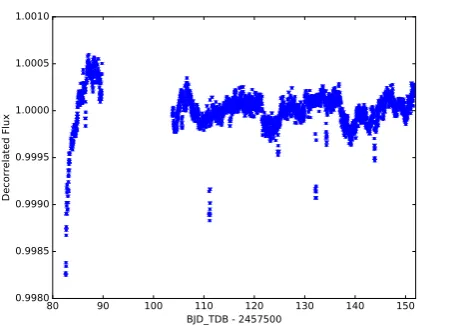
80 90 100 110 120 130 140 150 BJD_TDB - 2457500
0.9980 0.9985 0.9990 0.9995 1.0000 1.0005 1.0010
[image:4.595.50.278.65.228.2]Decorrelated Flux
Fig. 1. K2 detrended light curve of HD 106315 showing short term variability and two sets of transits.
2. Observations
2.1. K2 photometry
HD 106315 (EPIC 201437844) was observed during Campaign 10 of the K2 mission, in long cadence mode, between 2016 July 6 and 2016 September 20, spanning∼80 days. However, during the first six days of Campaign 10 there was a pointing error of 3.5-pixels preventing high precision photometry, so we did not reduce this data. Furthermore, on 2016 July 20 one of the mod-ules failed leading to the telescope going into safe mode and re-sulting in a 14-day gap in the observations. Therefore, Campaign 10 has slightly less data than previous campaigns. We down-loaded the pixel data from the Mikulski Archive for Space Tele-scopes (MAST).1 We reduced the pixel data and extracted the light curves using the Planet candidates from OptimaL Aperture Reduction (POLAR) pipeline. The POLAR pipeline has some routines that are part of the COnvection ROtation and plane-tary Transits (CoRoT) imagette pipeline (Barros et al. 2014). A full description of the POLAR pipeline is given in Barros et al. (2016). The POLAR reduced light curves up to Campaign 6 are publicly available through the MAST.2 The K2 light curve of HD 106315 is presented in Figure 1. The light curve is domi-nated by red noise due to granulation and we cannot find a clear rotation period. Moreover, the K2 light curve shows two sets of planetary signals that were previously reported by Crossfield et al. (2017) and Rodriguez et al. (2017). Planet b shows a transit depth of 297±34 ppm, while planet c shows a transit depth of 944±21 ppm. The phase folded transits of K2 for both planets, together with the best transit model presented in Section 5, are shown in Figure 2. The stellar-activity-filtered final light curve has a robust rms of 55ppm.
2.2. Follow-up photometry
In order to help constrain the orbital period and phase of HD 106315c, we monitored the transit on the night of 2017 March 8 from Cerro Tololo Inter-American Observatory (CTIO), Chile, with one of the three LCO (Las Cumbres Observatory) 1 m telescopes located at that site. LCO operates a network of fully automated 1 m telescopes (Brown et al. 2013) equipped with
1 htt ps://archive.stsci.edu/k2/data_search/search.php. 2 htt ps://archive.stsci.edu/prepds/polar/.
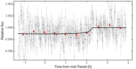
custom built imaging cameras (Sinistro3) with back-illuminated 4K×4K Fairchild Imaging CCDs (charged-coupled device) with 15µm pixels (CCD486 BI). With a plate scale of 0.387”/pixel, the Sinistro cameras deliver a field of view of 26.60×26.6 0, which is important for reference stars when monitoring bright stars such as HD 106315. The cameras are read out by four amplifiers with 1×1 binning, with a readout time of ≈ 45 s. We used thei-band filter, with exposure times of 30 s. Images were reduced by the standard LCO pipeline (Brown et al. 2013), and aperture photometry was performed in the manner set out in Penev et al. (2013). The phase folded light curve as well as the best fit model that we present in Section 5 are shown in Figure 3. The transit shows an egress with a depth and timing consistent with the predicted ephemeris from the K2 data.
2.3. HARPS radial velocity observations
We observed the target star HD 106315 with the HARPS spec-trograph, which is mounted on the ESO-3.6m telescope in La Silla Observatory (Chile), with the aim of detecting the mass of the two transiting planets. Since the star is relatively hot and fast-rotating, measuring precise radial velocities is challenging (Rodriguez et al. 2017). Crossfield et al. (2017) performed a first radial velocity follow-up of this target with the HiReS spectro-graph at the Keck telescope. They used exposure times of three to six minutes, and observed a large rms at the level of 6.4 m s−1. Hot stars are known to have large variability caused by granu-lation and p-modes (Dumusque et al. 2011). We estimated that p-modes have timescale of about 20 minutes, as in the case of Procyon (Bouchy et al. 2004). To average out the oscillation and granulation noises in the spectra, we used exposure times of 30 minutes and observed the target several times during the night with a few hours between exposures. We collected 93 spectra of HD 106315 with HARPS from 2017 January 26 to 2017 May 4, as part of our ESO-K2 large programme (Programme ID 198.C-0169). We rejected eight spectra because they were significantly affected by the Moon background light (Bonomo et al. 2010) or taken at high airmass (>1.7). We complemented our time series with 46 out-of-transit spectra taken as part of the HEARTS pro-gramme (Wyttenbach et al. 2017) on HARPS (propro-gramme ID 098.C-0304) during two transits of planet c. These data have an exposure time of five minutes during the first night and eight minutes during the second night. For this dataset we excluded observations that were taken with airmass higher than 1.7. All the HARPS spectra were reduced with the HARPS pipeline con-sistently. Radial velocities were derived by cross-correlating the spectra with a template of a G2V star (Baranne et al. 1996; Pepe et al. 2002). Radial velocity photon noise was estimated based on the work of Bouchy et al. (2001). We also measured the full width half maximum (FWHM) and the bisector inverse slope (BIS), and estimated their uncertainty as suggested in Santerne et al. (2015). All the radial velocity products are reported in Ta-ble .1. To mitigate the effect of stellar variability in the HEARTs data, for the final analysis we binned them to the same exposure time as the rest of the HARPS data (30 minutes), resulting in four points in the first night after the transit and four points in the second night before the transit.
We fitted the cross-correlation function with a rotation pro-file as described in Santerne et al. (2012) and derived a stellar
vsini=12.71±0.4 km s−1. This, combined with the stellar
ra-dius given in Table 2, gives a rotation period of 5.15±0.28d (if i=90). Using the SMWvalues and the calibration as described by
Fig. 2. Phase folded K2 light curve of HD 106315b (left panel) and HD 106315c (right panel). We overplot the best fitted model presented in Table 2
−1 0 1 2 3 4
Time from mid-Transit [h]
0.996 0.998 1.000 1.002 1.004
Relativ
e
flux
Fig. 3. Phase folded LCO light curve of HD 106315c taken with the i’ filter. We overplot the best fitted model presented in Table 2. We also overplot the binned light curve at 30 minute cadence. The residuals of the binned light curve show an rms of 219.0 ppm.
Noyes et al. (1984) and Lovis et al. (2011), we derived an activ-ity index of logR’HK=- 4.888±0.008. Given that the distance
to HD 106315 is higher than 100pc (Section 4), we checked whether interstellar clouds could be artificially decreasing the measured logR’HK. In our final fit we find a value for the
extinc-tion of 0.0049+0.008
−0.004mag; this value was confirmed by using the
galaxy maps by Green et al. (2015), which estimate the extinc-tion is lower than 0.01. Therefore, we do not expect a bias of the logR’HKgiven the low extinction.
The radial velocity observations show a clear variation phased with the fitted periods of the planets from the K2 pho-tometry. The HARPS RVs together with the best fit Keplerian model (section 5 ) are shown in Figure 4. In Figure 5, we show the periodogram of the residual of the radial velocities after sub-tracting the best fit model. We find no other significant peaks in the periodogram, and hence no other planet in the system is detected.
2.4. Lucky imaging
We observed HD 106315 with the high spatial resolution camera AstraLux (Hormuth et al. 2008) installed at the 2.2m telescope of Calar Alto Observatory (Almaría, Spain). This instrument ap-plies the lucky-imaging technique (Fried 1978) to avoid atmo-spheric distortions by obtaining thousands of short-exposure (be-low the atmospheric coherence time scale) images and selecting the best-quality ones based on the Strehl-ratio (Strehl 1902). In this case, we obtained 70 000 images of 30 ms exposure time in the SDSS (sloan digital sky survey) i-band and selected the best 10% of them. We used the observatory pipeline to perform the
basic reduction of the images, measure their Strehl ratio, select the best-quality frames, and finally align them and combine them to obtain the final high spatial resolution image. In this final im-age, we find no additional companions up to 12 arcsec within the sensitivity limits. In Figure 6 we show the sensitivity curve determined following the process explained in Lillo-Box et al. (2014), based on the injection of artificial stars into the image at different angular separations and position angles, and measuring the retrieved stars based on the same detection algorithms used to look for real companions.
Due to HD 106315 being saturated in K2, the best aper-ture used to extract the photometry is quite large, with a max-imum eight pixels in the x direction and 17 pixels in the y di-rection that correspond to 32x68 arcsec. Since this aperture is larger than the field of view of AstraLux (24x24 arcsec), we also checked for companions that could be inside the K2 aperture us-ing archival images. In Figure 7 we overlay the K2 aperture, the AstraLux image, and the SDSS r’ band image. Detected sources are marked with red circles in the image. We find a star at the edge of the K2 aperture (marked with a blue circle) that is 11 mag fainter than the target in the r’ band. Therefore, this star cannot be the source of the eclipses and has a negligible im-pact on the measurement of the planet radius (a correction of around 0.002%). Hence, our results confirm the non-detection of close-in companions to HD 106315 within 10 arcsec pre-sented by Crossfield et al. (2017), whose observations have a higher sensitivity closer to the target. We also exclude the ex-istence of significant contaminating stars present at larger dis-tances, but inside the K2 aperture. Ignoring the presence of all possible sources inside the photometric aperture can give rise to false positives (Cabrera et al. 2017).
3. Spectral analysis of the host star
In order to perform the spectral analysis of the host star we first co-added all the (Doppler corrected) individual spectra of HD 106315 into a single 1D spectra with IRAF (Image Reduc-tion and Analysis Facility).4 We found that the stellar param-eters derived with the equivalent width (EW) method (in our case ARES+MOOG, Sousa 2014) were not very reliable due to the fast rotation of the host star. In HD 106315 the fast ro-tation leads to a significant spectral line broadening that affects our spectral parameter retrieval method. Therefore, we adopted the values reported by Rodriguez et al. (2017) using the stellar
4 IRAF is distributed by National Optical Astronomy Observatories,
[image:5.595.52.281.242.358.2]780 790 800 810 820 830 840 850 860 870 880
Time [BJD-2 457 000]
−30 −20 −10 0 10 20
Radial
velocity
[m.s
−
1]
0.0 0.2 0.4 0.6 0.8 1.0
Orbital phase
−10 −5 0 5 10
Radial
velocity
[m.s
−
1]
0.0 0.2 0.4 0.6 0.8 1.0
Orbital phase
−10 −5 0 5 10
Radial
velocity
[m.s
−
[image:6.595.68.530.64.319.2]1]
[image:6.595.314.550.396.627.2]Fig. 4. Top panel: Time series of the radial velocities of HD 106315. Bottom panel: Radial velocities of HD 106315 phase folded on the ephemeris of planet b (left panel) and of planet c (right panel). For the phase folded plots, we show both data binned to 0.05 in phase (in red-dark) and unbinned data (grey). For all the cases, the errors include the estimated jitter added quadratically and we overplotted the best fitted model presented in Table 2, which includes the Gaussian process to model the activity. In the top panel we also show a model without GPs, which includes the two Keplerian orbits (dash-line).
Fig. 5. Periodogram of the residual of the radial velocities of HD 106315 after subtracting the best fit keplerian for planets b and c. The horizontal lines represent the false alarm probability at 0.1%, 1%, 10%, and 50% confidence level.
0 1 2 3 4 5 6
Angular separation (arcsec) −10
−8 −6 −4 −2 0
Contrast
(∆m,
mag)
Fig. 6. Contrast curve in the SDSS i-band for the neighbourhood of HD 106315.
−40 −30 −20 −10 0 10 20 30 40 α(arcsec)
−40 −30 −20 −10 0 10 20 30 40
δ
(a
rcsec)
N
E
[image:6.595.46.282.396.488.2]AstraLux SDSS r
Fig. 7. SDSS r’ band image of the field of HD 106315 with an inset showing the high spacial resolution image taken with AstraLux. Only one faint object (marked with a blue circle) is detected inside the K2 aperture (shadowed purple). The object is 11 magnitudes fainter than the main target and hence does not produce significant contamination.
parameter classification tool:Teff=6251±52 K, logg=4.1±0.1
[image:6.595.52.281.555.711.2]and fitted together with all the data we have for this system, in-cluding the modelling of the spectral energy distribution (SED) of the star and the stellar evolution tracks of Dartmouth (Dotter et al. 2008). From our combined analysis we obtained the final stellar parameters:Teff =6327±48 K , logg=4.252±4.252
0.043 [cgs] and [Fe/H] =-0.311± 0.079 dex. These parame-ters are naturally compatible with those adopted from Rodriguez et al. (2017).
These stellar parameters were used to derive the stellar chem-ical abundances, which for most of the elements were derived under the assumption of local thermodynamic equilibrium (LTE) using the 2014 version of the code MOOG (Sneden 1973) with
the abfind driver. For the lines affected by hyperfine splitting
(HFS), we used the blends driver. A grid of Kurucz ATLAS9 atmospheres (Kurucz 1993) was used as input along with the EWs and the atomic parameters, wavelength (λ), excitation en-ergy of the lower enen-ergy level (χ), and oscillator strength (loggf) of each line. The EWs of the different species lines were mea-sured automatically with the version 2 of the ARES programme5 (Sousa et al. 2007, 2015). However, due to the high rotation of the star, some of the stellar lines were blended. The EWs of these lines were measured manually with the tasksplotin IRAF. Abundances are measured from a few isolated lines and our pro-cedure is valid for these manually checked lines. As mentioned above, in this case the stellar parameter determination is not re-liable because it is a global fit. We refer the reader to the works of Adibekyan et al. (2012), Santos et al. (2015), and Delgado Mena et al. (2017) for further details and the complete line list. Li abundances were derived with the spectral synthesis method, also using the code MOOG and ATLAS atmosphere models as done in Delgado Mena et al. (2014). The derived chemical abun-dances are given in Table 1. We derive a stellar age of 3.4±2.5 Gyr using an empirical relation with [Y/Mg] (Tucci Maia et al. 2016), which is in good agreement with the age derived in Sec-tion 4 using stellar evoluSec-tion tracks.
4. Data analysis
We jointly analysed the HARPS radial velocities (RVs), the K2 light curve, the LCO light curve of HD 106315 and its SED as observed by the 2-MASS, Hipparcos, and wide-field infrared survey explorer (WISE)surveys (Munari et al. 2014; Høg et al. 2000; Cutri 2014) using the PASTIS software (Díaz et al. 2014; Santerne et al. 2015). Both planets HD 106315b and HD 106315c are modelled simultaneously. We analyse only sec-tions of the light curve centred at the mid-transit time of both planets and with a length of 2.5 transit durations. The RVs were modelled with Keplerian orbits and the transits were modelled with the JKTEBOP package (Southworth 2008), using an over-sampling factor of 30 for K2 to account for the long integration time of the data (Kipping 2010). The SED was modelled us-ing the BT-SETTL library of stellar atmospheres (Allard et al. 2012). This model was coupled with a Markov Chain Monte Carlo (MCMC) method with many different parallel Metropolis-Hastings chains (Díaz et al. 2014) to derive the system parame-ters and their uncertainties. At each step of the chains, the spec-troscopic stellar parameters were converted into physical pa-rameters (stellar mass and stellar radius) using the Darthmouth evolution tracks (Dotter et al. 2008). The coefficients of the quadratic limb-darkening law are also computed at each step of the chains using the stellar parameters and the tables of Claret &
5 The ARES code can be downloaded at
[image:7.595.304.532.85.384.2]http://www.astro.up.pt/∼sousasag/ares/.
Table 1.List of the abundances derived from the HARPS combined spectra of HD 106315.
Element Abundance Error Number of lines
dex dex
[CI/H] -0.13 0.03 2
[NaI/H] -0.13 0.04 2
[MgI/H] -0.26 0.11 2
[AlI/H] -0.25 0.04 2
[SiI/H] -0.11 0.04 13
[CaI/H] -0.11 0.04 9
[ScII/H] -0.29 0.04 4
[TiI/H] -0.18 0.08 14
[TiII/H] -0.23 0.04 5
[VI/H] -0.27 0.06 5
[CrI/H] -0.19 0.07 11
[CrII/H] -0.14 0.04 3
[MnI/H] -0.19 0.10 4
[CoI/H] -0.24 0.06 4
[NiI/H] -0.25 0.07 32
[CuI/H] -0.40 0.11 4
[ZnI/H] -0.32 0.1 3
[SrI/H] -0.19 0.08 1
[YII/H] -0.13 0.07 4
[ZrII/H] -0.19 0.05 4
[BaII/H] -0.08 0.07 3
[CeII/H] -0.22 0.07 3
[NdII/H] -0.35 0.11 4
A(Li)* 2.58 0.08 dex 1
*A(Li)=log[N(Li)/N(H)]+12
Bloemen (2011). Our choice of the limb-darkening treatment is motivated by the fact that the low cadence of the K2 data and the precision of the ground-based transit does not allow us to con-strain the limb-darkening coefficients. It was shown by Müller et al. (2013) that fixing the limb-darkening coefficients to the theoretical models is adequate in most cases and can be better than fitting them, especially for low-impact parameters. Based on Espinoza & Jordán (2015), we estimated that this procedure could bias the derived planet-to-star radius ratio by less than 1%, which is below our errors. We derive limb-darkening values of
u1 = 0.3024±0.0049 andu2 = 0.3057±0.0018 for the K2
light curve, andu1 =0.2270±0.004,u2 =0.3033±0.0018 for
the LCO light curve. We included a jitter parameter in the fit for each of the observation sets: K2 light curve, LCO light curve, and HARPS RVs. To model the possible effects of stellar activ-ity in the radial velocactiv-ity data, we used a Gaussian process (GP) with a quasi periodic kernel (Haywood et al. 2014). In this case the covariance matrix is defined as:
K=A2exp
−1 2 ∆t λ1 !2 −2
sinπP∆t
rot λ2 2 +I q
σ2+σ2
j. (1)
The first term is the quasi periodic kernel with the hyper-parameters: amplitude (A), rotation period (Prot), and two timescales (λ1, λ2 ). Finally,∆tis a matrix with elements∆ti j =
ti−tj. The second term is the identity matrix multiplied by usual data uncertaintiesσplus a jitter term to account for uncorrelated noiseσj.
(Gaia Collaboration et al. 2016b,a). As mentioned in the pre-vious section, for the effective temperature, the surface gravity, and metallicity we used normal priors centred on the values re-ported by Rodriguez et al. (2017). We also used normal priors for the orbital ephemeris centred on the values found by the de-tection pipeline and assuming a width of 0.08 d and 0.1 d for the period and transit epoch, respectively. For the orbital eccentric-ity, we chose aβdistribution as prior (Kipping 2013) and for the planet’s inclination we used a Sine distribution as prior (between 70◦and 90◦). For the remaining parameters we used uninforma-tive priors.
For the first exploration of the parameter space, we ran the MCMC with 20 chains of 3×10⁵ iterations each, with
start-ing points randomly drawn from the joint prior. We used a Kolmogorov-Smirnov test to reject non-converging chains (Díaz et al. 2014). In order to better explore the region of the parame-ter space close to the solution and derive accurate uncertainties, we ran a second MCMC with chains starting at the best solution found from the combination of the chains that converged. For this second MCMC, we ran 20 chains of 3×10⁵iterations. The
burn-in phase was removed before merging the converged chains to obtain the system parameters.
5. Results
The parameters derived by our model are given in Table 2. All the uncertainties provided in the table are statistical and they do not include unknown errors in the models. We reiterate that the stellar parameters presented in the table are derived from the combined analysis of the data and not from the spectral analysis. We derive the radius for both planets,rb=2.44±0.17R⊕and
rc=4.35±0.23 R⊕, which are in agreement with previously de-rived radii though closer to the values of Rodriguez et al. (2017) due to the scaling with the radius of the star. Since we used as pri-ors the stellar parameters derived by Rodriguez et al. (2017) and a similar data analysis method, their stellar radius is very close to our derived value while the value of Crossfield et al. (2017) is slightly smaller. Due to our high precision RVs, we were also able to derive precisely the mass of both planets:mb=12.6±3.2
M⊕andmc=15.2±3.7 M⊕. Therefore, the inner planet is much denser (4.7 ±1.7 g cm−3 ) than the outer planet (1.01 ±0.29 g cm−3). The ground-based transit obtained by LCO allows us to
update the ephemeris of HD 106315c, decreasing the uncertainty in the period by one order of magnitude. We find P=21.05704±
4.6×10⁻⁴days and T0=2457569.0173±1.4×10⁻³days, which
will help with future follow-up observations. We also find no significant transit timing variations.
The derived GP period is 2.825±0.012. This value is close to the half of the rotation period of the star derived fromvsini
assumingi=90. We find a similar periodicity in the FWHM in-dicating that this period is due to activity. However, the double of the period is not significant in the data. If this signal is due to ac-tivity, either the radial velocities show half the period of rotation of the star or the star has an inclination relative to the planetary orbit of∼30 degrees. Alternatively, the variability-induced sig-nal found in the RVs could be due to stellar super granulation, although the timescale of super granulation for this stellar type is expected to be lower.
To test the robustness of our results we redid all the anal-ysis using the stellar parameters from Crossfield et al. (2017). We found that all the derived values are within 1σ of our final values, which are based on stellar parameters from Rodriguez et al. (2017). We tested the existence of a linear, quadratic, and
cubic drift. Using the Bayesian information criterium, we con-clude that none of these drifts are significantly supported by the current data (∆BIC <5 comparing with no drift ). To further test the presence of this drift, we obtained an extra two HARPS radial velocities in early July 2017 (two months after the end of our intensive campaign) and still found no significant drift. These two points were ignored in our final analysis as they are completely uncorrelated with the intensive campaign. Crossfield et al. (2017) previously reported a hint of a drift of 0.3±0.1 m s−1day−1 ; this translates into 47 m s−1 over the 157 days of the total duration of our observations. Hence, the existence of this previously reported drift is also ruled out by our observa-tions.
6. Discussion and conclusions
To probe the composition of the two transiting planets orbiting HD 106315, we acquired high precision radial velocity observa-tions with the HARPS spectrograph. These observaobserva-tions allow us to derive a mass for both known planets orbiting HD 106315. We find that HD 106315b has a mass of 12.6±3.2 M⊕and a density of 4.7±1.7 g cm−3, while HD 106315c has a mass of 15.2±3.7 M⊕and a density of 1.01 ±0.29 g cm−3. This sys-tem embodies the diversity of planetary composition given that planet c is almost double the size of planet b although they have almost the same mass. Therefore, we expect they will have dif-ferent compositions.
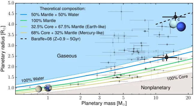
In Figure 8, we show the positions of HD 106315b and HD 106315c on the mass-radius diagram compared with known planets within the same mass and size range (M<20 M⊕and R <5 R⊕). To probe the planets’ composition, we plot in the same figure the theoretical models for solid planets with assumed compositions of pure iron, pure silicate, and pure water, as well as Earth-like and Mercury-like compositions (Brugger et al. sub-mitted). We also plot the model of Baraffe et al. (2008), which applies to planets with gaseous envelopes with a heavy material enrichment of 0.9 and an age of 5 Gyr, which appears to be a good match for HD 106315c. HD 106315b appears to be com-posed of a large fraction of silicate rocks and water.
Table 2.Physical parameters of the HD 106315 system.
Parameter Value and uncertainty
Orbital parameters HD 106315b HD 106315c
Orbital periodP[d] 9.55237±8.9×10⁻⁴ 21.05704±4.6×10⁻⁴
Epoch of first transit T0[BJDTDB- 2.4×10⁶] 57586.5487±2.9×10⁻³ 57569.0173±1.4×10⁻³
Orbital eccentricitye 0.093+0.110
−0.068 0.22±0.15
Argument of periastronω[◦] 239+74
−200 96+
88 −35
Semi-major axisa[AU] 0.0907±1.0×10⁻³ 0.1536±1.7×10⁻³
Inclinationi[◦] 87.54±0.32 88.61+0.70
−0.25
Transit&radial velocity parameters
System scalea/R? 15.07±0.70 25.5±1.2
Impact parameterb 0.67±0.1 0.52+0.17
−0.31
Transit duration T14[h] 3.775±0.081 4.638±0.072
Planet-to-star radius ratiokr 0.01728±6.0×10⁻⁴ 0.03086±0.0010
Radial velocity amplitudeK[ m s−1] 3.63±0.92 3.43±0.83
Planet parameters
Planet massMp[M⊕] 12.6±3.2 15.2±3.7
Planet radiusRp[R⊕] 2.44±0.17 4.35±0.23
Planet densityρp[g cm−3] 4.7±1.7 1.01±0.29
Equilibrium temperatureTeq[K] 1153±25 886±20
Stellar parameters
Stellar massM?[M] 1.091±0.036
Stellar radiusR?[R] 1.296±0.058
Stellar ageτ[Gyr] 4.48±0.96
Effective temperatureTeff[K] 6327±48
Surface gravity logg[g cm−2] 4.252±0.043
Iron abundance [Fe/H] [dex] -0.311±0.079
Reddening E(B-V) [mag] 0.0050+0.0085
−0.0038
Systemic radial velocityυ0[ km s−1] -3.34+−00..5638
Distance to Earthd[pc] 109±5
Spectral type F5V
Instrumental parameters
HARPS radial velocity jitter [ m s−1] 3.05±0.78
SED jitter [mag] 0.079±0.020
K2jitter [ppm] 44±2
K2contamination [ppt] 3.3+3.8
−2.3
K2flux normalisation 1.000001±3.1×10⁻⁶
LCO jitter [ppt] 1.424±0.065
LCO contamination 0.1+0.12
−0.07
LCO flux normalisation 0.99994±0.00011
GP period [d] 2.825±0.012
GP amplitude [ m s−1] 0.57±0.35
GPλ1[d] 652.5±340
GPλ2 299.0±260
We assumed R=695 508km, M=1.98842×1030kg, R⊕=6 378 137m, M⊕=5.9736×1024kg, and 1AU=149 597 870.7km.
of HD 106315b is found to be in the range 0–52%. Given the uncertainties on the fundamental parameters of this planet, its core mass and water fraction cannot be better constrained.
b c
1 2 3 5 10 20
Planetary mass [M⊕] 1.0
1.5 2.0 2.5 3.0 3.5 4.0 4.5 5.0
Planetar y radius [R⊕ ] 100% Core 100% Water Nonplanetary Gaseous Theoretical composition: 50% Mantle + 50% Water 100% Mantle
32.5% Core + 67.5% Mantle (Earth-like) 68% Core + 32% Mantle (Mercury-like)
Baraffe+08 (Z=0.9 – 5Gyr) Fig. 8. Mass-radius relationship for diff
er-ent bulk compositions of small planets. We overplot different compositions for solid plan-ets in between pure iron and pure water. The black dashed line corresponds to the models of Baraffe et al. (2008) for gaseous planets with heavy material enrichments of 0.9 and an age of 5 Gyr. We superimposed the known planets in this mass-radius range where the greyscale depends on the precision of the mass and radius. We mark the position of the planets HD 106315b and HD 106315c, as derived by us.
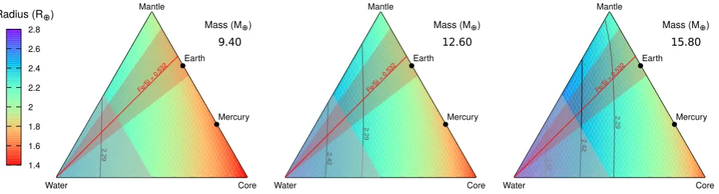
the stellar abundances from Section 3, we compute that Fe/Si= 0.532± 0.316. Here, incorporating this parameter in the inte-rior model gives a 9-50% range for the water mass fraction and 5-29% for the core mass fraction. It appears that HD 106315b cannot be fully rocky and must harbour a significant water en-velope. Both the water mass fraction and the core mass fraction of this planet can be significantly constrained via the use of the stellar Fe/Si ratio and the limitations from solar system forma-tion condiforma-tions, respectively.
The other possibility is that HD 106315b is composed of a rocky core with a thick H-He envelope. This could be expected since HD 106315b is close to the transition between rocky and gaseous planets. HD 106315b and c have the potential to bring light to this transition, given their close masses but different radii. To probe the evolution of this interesting multi-planetary sys-tem, we compared our derived systems parameters with the re-sults of synthetic planetary populations and evolutionary tracks calculated with the Bern model of planet formation and evolu-tion (Alibert et al. 2005; Mordasini et al. 2012; Benz et al. 2014) available through DACE6 (Data and Analysis Center for
Exo-planets). The simulations assume a stellar mass of 1M, a stellar age of 4Gyr, and cold gas accretion. The long-term evolution ne-glects envelope evaporation. We compared simulations with sim-ilar semi-major axis and mass to the values we derived for both the planets. All simulations have a semi-major axis higher than 0.101 AU. Therefore they cannot reproduce planet b. However, using the simulation with semi-major axis∼0.101 AU as proxy for planet b, we find that this planet could have been formed in between 0.11 and 2.5 AU and probably has a core mass just slightly lower (∼12M⊕) than the total planetary mass. We found a close proxy for planet c, which suggests that it could have been formed between 1.0 and 3.0 AU. Hence, in general planet c formed further away from the host star than planet b and is expected to have similar core mass (∼12M⊕). Another interest-ing fact is that the predicted radius for both planets is almost the same and in agreement with the value we measured for planet c. However, the radii of the simulated planets are always higher than the radius of planet b. This could be explained if planet b, as it lies closer to the host star, has suffered envelope evaporation, which is not taken into account in the simulation. Therefore, the difference in the density between both planets can be explained by the different formation region in the proto-planetary disc as well as a possible envelope evaporation.
6 https://dace.unige.ch.
With Equation 15 of Lecavelier Des Etangs (2007), we esti-mate the escape rate of the atmosphere using two different val-ues for theFEUV (1AU): 14.7 erg cm−2s−1from Lecavelier Des Etangs (2007) and 82.76 erg cm−2s−1calculated using Equation
3 of Ehrenreich & Désert (2011). Assuming that theFEUV(1AU) is constant, we calculate an atmosphere loss of∼[ 0.018, 0.10] earth masses for planet b and∼[0.033, 0.19] for planet c dur-ing their lifetime of 4 Gyr. Therefore, it appears that the mass loss is not important for these two planets. However, our first approximation of the mass loss rates should be confirmed with more detailed models of evaporating atmospheres, which are out of the scope of this paper.
Gaining insight into the composition of the atmosphere of these planets would allow us to better constrain their interior composition and their formation history. We estimate the scale height of the atmosphere of HD 106315b and HD 106315c to be
∼196.72 Km and∼464.53 Km, respectively. Therefore, given the brightness of the host star, both planets are also golden tar-gets for transmission spectroscopy with JWST. This would be particularly interesting for HD 106315b since this planet lies in the transition between rocky and gaseous planet composition. Probing its atmosphere with upcoming new facilities like JWST and the extremely large telescopes (ELTs) will help to better un-derstand the composition of this planet.
[image:10.595.45.369.60.238.2]Water Core Mantle
Earth
Mercury Radius (R⊕)
Mass (M⊕)
9.40 1.4 1.6 1.8 2 2.2 2.4 2.6 2.8
Fe/Si = 0.532
2.29
Water Core
Mantle
Earth
Mercury
Mass (M⊕)
12.60
Fe/Si = 0.532
2.29 2.42 Water Core Mantle Earth Mercury
Mass (M⊕)
15.80
Fe/Si = 0.532
2.29
2.42
[image:11.595.43.555.56.194.2]2.55
Fig. 9.Ternary diagrams displaying the investigated compositional parameter space of HD 106315b for the minimum, central, and maximum masses, using 1σuncertainties. Also shown are the isoradius curves denoting the planet radius with the 1σextreme values. The planetary Fe/Si ratio assumed for HD 106315b, with its associated 1σuncertainties, delimits an area represented as a red triangle. Planetary compositions with a water mass fraction higher than 50% are excluded, based on assumptions on the solar system’s present properties (grey zone).
by these grants UID/FIS/04434/2013 & POCI-01-0145-FEDER-007672 , PTDC/FIS-AST/1526/2014 & POCI-01-0145-FEDER-016886 and PTDC/ FIS-AST/7073/2014 & POCI-01-0145-FEDER-016880. SCCB, E.D.M. V.Zh.A., N.C.S., PF, and S.G.S. also acknowledge support from FCT through In-vestigador FCT contracts IF/01312/2014/CP1215/CT000, IF/00849/2015, IF/00650/2015/CP1273/CT0001, IF/00169/2012/CP0150/CT0002, IF/01037/2013/CP1191/CT0001 and IF/00028/2014/CP1215/CT0002 funded by FCT (Portugal) and POPH/FSE (EC). VZhA and JPF also acknowledge support from the FCT in the form of the grants SFRH/BPD/70574/2010 and SFRH/BD/93848/2013, respectively. PF further acknowledges support from Fundação para a Ciência e a Tecnologia (FCT) through POPH/FSE (EC) by FEDER funding through the programme “Programa Operacional de Factores de Competitividade - COMPETE” and exploratory project of reference IF/01037/2013/CP1191/CT0001. J.P.F., S.H., and J.J.N. acknowledge support by the fellowships SFRH/BD/93848/2013, PD/BD/128119/2016, and PD/BD/52700/2014, funded by FCT (Portugal) and POPH/FSE (EC). The French group acknowledges financial support from the French Programme National de Planétologie (PNP, INSU). The Swiss group acknowledges financial support the National Centre for Competence in Research "PlanetS" supported by the Swiss National Science Foundation (SNSF). DJA is funded under STFC consolidated grant reference ST/P000495/1. This work has been partly carried out thanks to support funding from Excellence Initiative of Aix-Marseille University A*MIDEX, a French "Investissements d’Avenir" programme. ACC acknowledges support from STFC consolidated grant number ST/M001296/1. XD is grateful to the Society in Science? The Branco Weiss Fellowship for its financial support. Part of this research has been funded by the Spanish grant ESP2015-65712-C5-1-R. We thank the anonymous referee for the careful review of this manuscript that improved its quality.
References
Adibekyan, V. Z., Sousa, S. G., Santos, N. C., et al. 2012, A&A, 545, A32 Albrecht, S., Winn, J. N., Johnson, J. A., et al. 2012, ApJ, 757, 18 Alibert, Y. 2014, A&A, 561, A41
Alibert, Y., Mordasini, C., Benz, W., & Winisdoerffer, C. 2005, A&A, 434, 343 Allard, F., Homeier, D., & Freytag, B. 2012, Royal Society of London
Philo-sophical Transactions Series A, 370, 2765
Baraffe, I., Chabrier, G., & Barman, T. 2008, A&A, 482, 315 Baranne, A., Queloz, D., Mayor, M., et al. 1996, A&AS, 119, 373 Barclay, T., Rowe, J. F., Lissauer, J. J., et al. 2013, Nature, 494, 452 Barros, S. C. C., Almenara, J. M., Deleuil, M., et al. 2014, A&A, 569, A74 Barros, S. C. C., Demangeon, O., & Deleuil, M. 2016, A&A, 594, A100 Batalha, N. E., Kempton, E. M.-R., & Mbarek, R. 2017, ApJ, 836, L5 Benz, W., Ida, S., Alibert, Y., Lin, D., & Mordasini, C. 2014, Protostars and
Planets VI, 691
Bonomo, A. S., Santerne, A., Alonso, R., et al. 2010, A&A, 520, A65 Borucki, W. J., Koch, D., Basri, G., et al. 2010, Science, 327, 977 Bouchy, F., Maeder, A., Mayor, M., et al. 2004, Nature, 432, 2 Bouchy, F., Pepe, F., & Queloz, D. 2001, A&A, 374, 733
Brown, T. M., Baliber, N., Bianco, F. B., et al. 2013, PASP, 125, 1031 Cabrera, J., Barros, S. C. C., Armstrong, D., et al. 2017, ArXiv e-prints
[arXiv:1707.08007]
Carter, J. A., Agol, E., Chaplin, W. J., et al. 2012, Science, 337, 556
Claret, A. & Bloemen, S. 2011, A&A, 529, A75+
Crossfield, I. J. M., Ciardi, D. R., Isaacson, H., et al. 2017, AJ, 153, 255 Cutri, R. M. 2014, VizieR Online Data Catalog, 2328
Delgado Mena, E., Israelian, G., González Hernández, J. I., et al. 2014, A&A, 562, A92
Delgado Mena, E., Tsantaki, M., Adibekyan, V. Z., et al. 2017, ArXiv e-prints
[arXiv:1705.04349]
Díaz, R. F., Almenara, J. M., Santerne, A., et al. 2014, MNRAS, 441, 983 Dotter, A., Chaboyer, B., Jevremovi´c, D., et al. 2008, ApJS, 178, 89 Dressing, C. D., Charbonneau, D., Dumusque, X., et al. 2015, ApJ, 800, 135 Dumusque, X., Bonomo, A. S., Haywood, R. D., et al. 2014, ApJ, 789, 154 Dumusque, X., Udry, S., Lovis, C., Santos, N. C., & Monteiro, M. J. P. F. G.
2011, A&A, 525, A140
Ehrenreich, D. & Désert, J.-M. 2011, A&A, 529, A136 Espinoza, N. & Jordán, A. 2015, MNRAS, 450, 1879 Ford, E. B. & Rasio, F. A. 2008, ApJ, 686, 621
Fressin, F., Torres, G., Charbonneau, D., et al. 2013, ApJ, 766, 81
Fried, D. L. 1978, Journal of the Optical Society of America (1917-1983), 68, 1651
Fulton, B. J., Petigura, E. A., Howard, A. W., et al. 2017, ArXiv e-prints
[arXiv:1703.10375]
Gaia Collaboration, Brown, A. G. A., Vallenari, A., et al. 2016a, A&A, 595, A2 Gaia Collaboration, Prusti, T., de Bruijne, J. H. J., et al. 2016b, A&A, 595, A1 Green, G. M., Schlafly, E. F., Finkbeiner, D. P., et al. 2015, ApJ, 810, 25 Haywood, R. D., Collier Cameron, A., Queloz, D., et al. 2014, MNRAS, 443,
2517
Høg, E., Fabricius, C., Makarov, V. V., et al. 2000, A&A, 355, L27
Hormuth, F., Brandner, W., Hippler, S., & Henning, T. 2008, Journal of Physics Conference Series, 131, 012051
Howell, S. B., Sobeck, C., Haas, M., et al. 2014, PASP, 126, 398
Jontof-Hutter, D., Rowe, J. F., Lissauer, J. J., Fabrycky, D. C., & Ford, E. B. 2015, Nature, 522, 321
Kipping, D. M. 2010, MNRAS, 408, 1758 Kipping, D. M. 2013, MNRAS, 434, L51
Kurucz, R. 1993, ATLAS9 Stellar Atmosphere Programs and 2 km/s grid. Ku-rucz CD-ROM No. 13. Cambridge, Mass.: Smithsonian Astrophysical Ob-servatory, 1993., 13
Lecavelier Des Etangs, A. 2007, A&A, 461, 1185 Léger, A., Selsis, F., Sotin, C., et al. 2004, Icarus, 169, 499 Lillo-Box, J., Barrado, D., & Bouy, H. 2014, A&A, 566, A103 Lissauer, J. J. 1993, ARA&A, 31, 129
Lissauer, J. J., Fabrycky, D. C., Ford, E. B., et al. 2011, Nature, 470, 53 Lovis, C., Dumusque, X., Santos, N. C., et al. 2011, ArXiv e-prints
[arXiv:1107.5325]
Malavolta, L., Borsato, L., Granata, V., et al. 2017, AJ, 153, 224 Marcy, G. W., Isaacson, H., Howard, A. W., et al. 2014, ApJS, 210, 20 Mayor, M., Marmier, M., Lovis, C., et al. 2011, ArXiv e-prints
[arXiv:1109.2497]
Mayor, M., Pepe, F., Queloz, D., et al. 2003, The Messenger, 114, 20 McLaughlin, D. B. 1924, ApJ, 60, 22
Mordasini, C., Alibert, Y., Klahr, H., & Henning, T. 2012, A&A, 547, A111 Müller, H. M., Huber, K. F., Czesla, S., Wolter, U., & Schmitt, J. H. M. M. 2013,
A&A, 560, A112
Munari, U., Henden, A., Frigo, A., et al. 2014, AJ, 148, 81 Nayakshin, S. 2017, PASA, 34, e002
Penev, K., Bakos, G. Á., Bayliss, D., et al. 2013, AJ, 145, 5 Pepe, F., Mayor, M., Galland, F., et al. 2002, A&A, 388, 632 Rasio, F. A. & Ford, E. B. 1996, Science, 274, 954
Rodriguez, J. E., Zhou, G., Vanderburg, A., et al. 2017, ArXiv e-prints
[arXiv:1701.03807]
Rogers, L. A. 2015, ApJ, 801, 41
Rogers, L. A., Bodenheimer, P., Lissauer, J. J., & Seager, S. 2011, ApJ, 738, 59 Rossiter, R. A. 1924, ApJ, 60, 15
Santerne, A., Díaz, R. F., Almenara, J.-M., et al. 2015, MNRAS, 451, 2337 Santerne, A., Moutou, C., Barros, S. C. C., et al. 2012, A&A, 544, L12 Santos, N. C., Adibekyan, V., Mordasini, C., et al. 2015, A&A, 580, L13 Seager, S., Kuchner, M., Hier-Majumder, C. A., & Militzer, B. 2007, ApJ, 669,
1279
Sneden, C. A. 1973, PhD thesis, The University of Texas at Austin.
Sousa, S. G. 2014, ARES+MOOG: A Practical Overview of an Equivalent Width (EW) Method to Derive Stellar Parameters, ed. E. Niemczura, B. Smal-ley, & W. Pych, 297–310
Sousa, S. G., Santos, N. C., Adibekyan, V., Delgado-Mena, E., & Israelian, G. 2015, A&A, 577, A67
Sousa, S. G., Santos, N. C., Israelian, G., Mayor, M., & Monteiro, M. J. P. F. G. 2007, A&A, 469, 783
Southworth, J. 2008, MNRAS, 386, 1644
Strehl, K. 1902, Astronomische Nachrichten, 158, 89
Thiabaud, A., Marboeuf, U., Alibert, Y., Leya, I., & Mezger, K. 2015, A&A, 580, A30
Tucci Maia, M., Ramírez, I., Meléndez, J., et al. 2016, A&A, 590, A32 Valencia, D., O’Connell, R. J., & Sasselov, D. 2006, Icarus, 181, 545 Weidenschilling, S. J. & Marzari, F. 1996, Nature, 384, 619 Weiss, L. M. & Marcy, G. W. 2014, ApJ, 783, L6
Winn, J. N., Fabrycky, D., Albrecht, S., & Johnson, J. A. 2010, ApJ, 718, L145 Wyttenbach, A., Lovis, C., Ehrenreich, D., et al. 2017, ArXiv e-prints
Table .2.List of free parameters used in thePASTISanalysis of the light curves, radial velocities, and SED with their associated prior and posterior distribution.
Parameter Prior Posterior
Orbital parameters
HD 106315b
Orbital periodP[d] N(9.552; 0.081) 9.55236±8.8×10⁻⁴
Epoch of first transit T0[BJDTDB- 2.4×10⁶] N(57586.5; 0.1) 57586.5486±2.9×10⁻³
Orbital eccentricitye β(0.867; 3.030) 0.078+0.110
−0.059
Argument of periastronω[◦] U(0; 360) 245+69
−190
Inclinationi[◦] S(70; 90) 87.57±0.28
HD 106315c
Orbital periodP[d] N(21.05; 0.20) 21.05704±4.3×10⁻⁴
Epoch of first transit T0[BJDTDB- 2.4×10⁶] N(57569.0; 0.15) 57569.0173±1.4×10⁻³
Orbital eccentricitye β(0.867; 3.030) 0.22±0.16
Argument of periastronω[◦] U(0; 360) 81+47
−32
Inclinationi[◦] S(70; 90) 88.66+0.84
−0.26
Planetary parameters
HD 106315b
Radial velocity amplitudeK[ m s−1] U(0; 1000) 3.79±0.92
Planet-to-star radius ratiokr U(0; 1) 0.01725±5.1×10⁻⁴ HD 106315c
Radial velocity amplitudeK[ m s−1] U(0; 1000) 3.11±0.80
Planet-to-star radius ratiokr U(0; 1) 0.03073+−00..0010000069
Stellar parameters
Effective temperatureTeff[K] N(6251; 52) 6332±51
Surface gravity logg[g cm−2] N(4.1; 0.1) 4.258±0.036
Iron abundance [Fe/H] [dex] N(−0.27; 0.08) -0.314±0.078
Reddening E(B-V) [mag] U(0; 0.1) 0.0049+0.0080
−0.0035
Systemic radial velocityυ0[ km s−1] U(−10; 5) -3.4648±6.9×10⁻⁴
Distance to Earthd[pc] N(107.3; 3.9) 108±4
Instrumental parameters
HARPS radial velocity jitter [ m s−1] U(0; 1000) 2.89±0.72
SED jitter [mag] U(0; 1) 0.078±0.021
K2jitter [ppm] U(0; 10000) 44±2
K2contamination [ppt] NU(0; 5; 0; 1000) 3.3+−32..83 K2flux normalisation U(0.999; 1.001) 1.000001±3.1×10⁻⁶
LCO jitter [ppt] U(0; 100) 1.422±0.065
LCO contamination U(0; 1) 0.10+0.12
−0.07
LCO flux normalisation U(0.99; 1.01) 0.99994±0.00011
GP period [d] U(0; 8) 2.825±0.012
GP amplitude [ m s−1] U(0; 1) 0.57±0.35
GPλ1[d] U(0; 1000) 652.5±340
GPλ2 U(0; 1000) 299.0±260
N(µ;σ2) is a normal distribution with meanµand widthσ2,U(a;b) is a uniform distribution betweenaandb,NU(µ;σ2,a,b) is a normal distribution with meanµand widthσ2multiplied with a uniform distribution betweenaandb,S(a,b) is a sine distribution
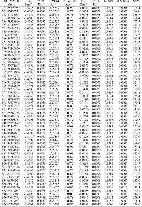
Table .1.List of the HARPS radial velocity observations of HD 106315 as well as the activity indicators.
BJD - 2457000 RV σRV FWHM σFWHM BIS σBIS S index σS index SN50
days Km−1 Km−1 Km−1 Km−1 Km−1 Km−1
781.85390953 -3.4735 0.0046 20.5547 0.0093 -0.0044 0.0093 0.1614 0.0008 126.4
782.87436772 -3.4633 0.0040 20.5316 0.0079 0.0075 0.0079 0.1600 0.0007 90.4
783.81136007 -3.4673 0.0037 20.5878 0.0075 -0.0375 0.0075 0.1615 0.0006 158.7
783.88784226 -3.4603 0.0037 20.5069 0.0073 -0.0153 0.0073 0.1604 0.0006 164.4
784.79328906 -3.4562 0.0037 20.5735 0.0075 -0.0081 0.0075 0.1611 0.0006 157.9
784.87188935 -3.4625 0.0035 20.5983 0.0071 0.0012 0.0071 0.1595 0.0006 171.8
785.79689773 -3.4694 0.0038 20.5106 0.0076 -0.0099 0.0076 0.1610 0.0006 153.6
785.88564972 -3.4747 0.0037 20.5331 0.0073 0.0210 0.0073 0.1608 0.0006 164.0
786.82325003 -3.4638 0.0036 20.5963 0.0072 -0.0199 0.0072 0.1598 0.0006 164.2
786.88285465 -3.4655 0.0034 20.5831 0.0068 0.0331 0.0068 0.1605 0.0005 177.4
787.75881115 -3.4654 0.0043 20.5866 0.0085 -0.0343 0.0085 0.1622 0.0006 134.5
787.85438149 -3.4750 0.0045 20.5698 0.0090 0.0034 0.0090 0.1636 0.0007 128.6
789.77546920 -3.4745 0.0040 20.5644 0.0080 0.0010 0.0080 0.1621 0.0006 143.5
789.85344400 -3.4727 0.0037 20.5702 0.0075 -0.0089 0.0075 0.1620 0.0006 157.7
790.80660507 -3.4737 0.0036 20.5956 0.0072 0.0072 0.0072 0.1606 0.0005 162.2
790.88801699 -3.4656 0.0036 20.5609 0.0072 0.0105 0.0072 0.1616 0.0006 169.2
791.78669995 -3.4672 0.0038 20.5483 0.0077 0.0334 0.0077 0.1626 0.0006 149.9
791.87071697 -3.4699 0.0036 20.5499 0.0072 -0.0177 0.0072 0.1622 0.0006 166.8
792.78409886 -3.4582 0.0034 20.5411 0.0068 -0.0064 0.0068 0.1621 0.0005 171.8
792.85214066 -3.4589 0.0034 20.5711 0.0068 -0.0066 0.0068 0.1617 0.0005 176.7
795.74546592 -3.4534 0.0040 20.5601 0.0080 -0.0066 0.0080 0.1602 0.0006 141.2
795.84097630 -3.4599 0.0038 20.5616 0.0075 0.0137 0.0075 0.1630 0.0006 154.9
796.75138530 -3.4668 0.0037 20.5390 0.0075 0.0222 0.0075 0.1622 0.0005 154.1
796.85387600 -3.4591 0.0038 20.5296 0.0076 0.0130 0.0076 0.1657 0.0006 154.1
797.76222264 -3.4589 0.0038 20.5069 0.0077 0.0430 0.0077 0.1622 0.0006 150.0
797.87625292 -3.4676 0.0036 20.4928 0.0072 0.0111 0.0072 0.1607 0.0006 167.2
801.78821294 -3.4649 0.0038 20.5511 0.0075 0.0033 0.0075 0.1614 0.0006 155.4
801.89787829 -3.4701 0.0051 20.5682 0.0103 0.0190 0.0103 0.1618 0.0009 114.4
802.75056942 -3.4692 0.0036 20.5470 0.0072 0.0131 0.0072 0.1619 0.0005 160.2
802.86325582 -3.4621 0.0040 20.5395 0.0080 0.0186 0.0080 0.1616 0.0007 147.6
803.72859542 -3.4542 0.0043 20.5558 0.0087 -0.0240 0.0087 0.1621 0.0007 131.0
803.85760258 -3.4637 0.0036 20.5883 0.0072 0.0270 0.0072 0.1611 0.0006 166.5
810.72887134 -3.4693 0.0045 20.5705 0.0090 0.0264 0.0090 0.1597 0.0007 128.0
810.79508131 -3.4661 0.0036 20.5319 0.0072 0.0132 0.0072 0.1603 0.0006 166.5
810.85053677 -3.4653 0.0036 20.5459 0.0072 0.0231 0.0072 0.1607 0.0006 166.6
814.72562795 -3.4644 0.0034 20.5097 0.0068 -0.0087 0.0068 0.1595 0.0005 171.6
814.78416320 -3.4584 0.0035 20.5319 0.0070 -0.0152 0.0070 0.1592 0.0006 170.2
814.85467687 -3.4590 0.0039 20.5821 0.0078 -0.0269 0.0078 0.1582 0.0007 152.7
815.70791294 -3.4626 0.0035 20.5883 0.0070 0.0223 0.0070 0.1593 0.0005 167.6
815.78306872 -3.4602 0.0036 20.6120 0.0071 0.0030 0.0071 0.1606 0.0006 168.1
815.86244959 -3.4603 0.0033 20.5888 0.0066 0.0110 0.0066 0.1592 0.0006 189.6
816.87984898 -3.4603 0.0046 20.5048 0.0091 0.0251 0.0091 0.1617 0.0009 131.4
817.70931545 -3.4640 0.0039 20.5688 0.0079 -0.0138 0.0079 0.1614 0.0006 148.6
817.77900779 -3.4581 0.0034 20.5740 0.0069 -0.0283 0.0069 0.1600 0.0006 173.0
817.84788906 -3.4636 0.0034 20.5545 0.0069 -0.0199 0.0069 0.1600 0.0006 177.8
820.76823244 -3.4646 0.0036 20.5824 0.0071 -0.0200 0.0071 0.1603 0.0006 170.9
820.87233534 -3.4556 0.0036 20.5720 0.0072 0.0063 0.0072 0.1594 0.0007 171.7
822.70228346 -3.4661 0.0042 20.5272 0.0083 0.0189 0.0083 0.1605 0.0007 140.7
822.81967340 -3.4632 0.0038 20.5155 0.0076 0.0195 0.0076 0.1598 0.0006 159.9
823.82120368 -3.4600 0.0033 20.6031 0.0066 0.0154 0.0066 0.1589 0.0006 187.6
831.68738142 -3.4571 0.0037 20.5936 0.0074 -0.0057 0.0074 0.1612 0.0006 164.4
834.66790071 -3.4617 0.0044 20.5143 0.0088 0.0019 0.0088 0.1597 0.0007 135.0
836.68938313 -3.4578 0.0049 20.5885 0.0098 0.0556 0.0098 0.1637 0.0009 121.6
837.65953470 -3.4653 0.0053 20.6056 0.0105 0.0137 0.0105 0.1631 0.0010 113.3
838.65577061 -3.4664 0.0038 20.5938 0.0076 -0.0095 0.0076 0.1585 0.0007 160.1
840.62130041 -3.4499 0.0051 20.4929 0.0103 -0.0189 0.0103 0.1620 0.0009 114.5
840.71047795 -3.4653 0.0039 20.5675 0.0078 -0.0016 0.0078 0.1612 0.0007 159.3
843.63219053 -3.4581 0.0043 20.5393 0.0087 -0.0127 0.0087 0.1598 0.0007 136.4
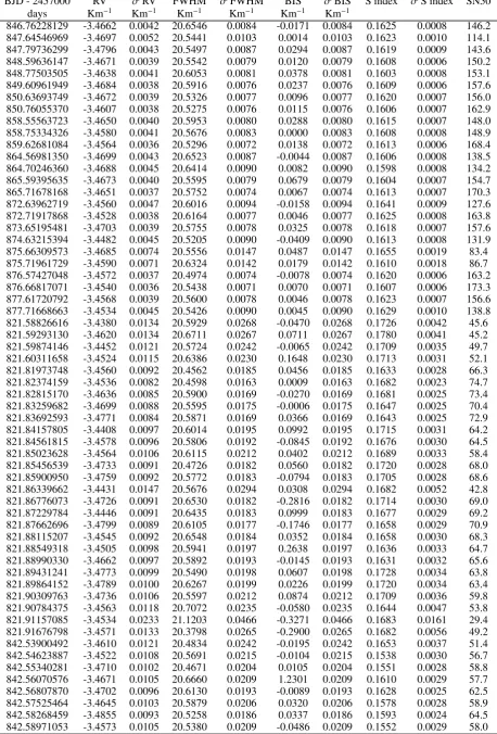
Table .1.Continued.
BJD - 2457000 RV σRV FWHM σFWHM BIS σBIS S index σS index SN50
days Km−1 Km−1 Km−1 Km−1 Km−1 Km−1
846.76228129 -3.4662 0.0042 20.6546 0.0084 -0.0171 0.0084 0.1625 0.0008 146.2
847.64546969 -3.4697 0.0052 20.5441 0.0103 0.0014 0.0103 0.1623 0.0010 114.1
847.79736299 -3.4796 0.0043 20.5497 0.0087 0.0294 0.0087 0.1619 0.0009 143.6
848.59636147 -3.4671 0.0039 20.5542 0.0079 0.0120 0.0079 0.1608 0.0006 150.2
848.77503505 -3.4638 0.0041 20.6053 0.0081 0.0378 0.0081 0.1603 0.0008 153.1
849.60961949 -3.4684 0.0038 20.5916 0.0076 0.0237 0.0076 0.1609 0.0006 157.6
850.63693749 -3.4672 0.0039 20.5326 0.0077 0.0096 0.0077 0.1620 0.0007 156.0
850.76055370 -3.4607 0.0038 20.5275 0.0076 0.0115 0.0076 0.1606 0.0007 162.9
858.55563723 -3.4650 0.0040 20.5953 0.0080 0.0288 0.0080 0.1615 0.0007 148.0
858.75334326 -3.4580 0.0041 20.5676 0.0083 0.0000 0.0083 0.1608 0.0008 148.9
859.62681084 -3.4564 0.0036 20.5296 0.0072 0.0138 0.0072 0.1613 0.0006 168.4
864.56981350 -3.4699 0.0043 20.6523 0.0087 -0.0044 0.0087 0.1606 0.0008 138.5
864.70246360 -3.4688 0.0045 20.6414 0.0090 0.0082 0.0090 0.1598 0.0008 134.2
865.59395635 -3.4673 0.0040 20.5595 0.0079 0.0679 0.0079 0.1604 0.0007 154.7
865.71678168 -3.4651 0.0037 20.5752 0.0074 0.0067 0.0074 0.1613 0.0007 170.3
872.63962719 -3.4560 0.0047 20.6016 0.0094 -0.0158 0.0094 0.1641 0.0009 127.6
872.71917868 -3.4528 0.0038 20.6164 0.0077 0.0046 0.0077 0.1625 0.0008 163.8
873.65195481 -3.4703 0.0039 20.5755 0.0078 0.0325 0.0078 0.1618 0.0007 157.6
874.63215394 -3.4482 0.0045 20.5205 0.0090 -0.0409 0.0090 0.1613 0.0008 131.9
875.66309573 -3.4685 0.0074 20.5556 0.0147 0.0487 0.0147 0.1655 0.0019 83.4
875.71961729 -3.4590 0.0071 20.6324 0.0142 0.0179 0.0142 0.1610 0.0018 86.7
876.57427048 -3.4572 0.0037 20.4974 0.0074 -0.0078 0.0074 0.1620 0.0006 163.2
876.66817071 -3.4540 0.0036 20.5438 0.0071 0.0070 0.0071 0.1607 0.0006 173.3
877.61720792 -3.4568 0.0039 20.5600 0.0078 0.0046 0.0078 0.1623 0.0007 156.6
877.71668663 -3.4534 0.0045 20.5426 0.0090 0.0045 0.0090 0.1629 0.0010 138.8
821.58826616 -3.4380 0.0134 20.5929 0.0268 -0.0470 0.0268 0.1726 0.0042 45.6
821.59293130 -3.4620 0.0134 20.6711 0.0267 0.0711 0.0267 0.1780 0.0041 45.2
821.59874146 -3.4452 0.0121 20.5724 0.0242 -0.0065 0.0242 0.1709 0.0035 49.7
821.60311658 -3.4524 0.0115 20.6386 0.0230 0.1648 0.0230 0.1713 0.0031 52.1
821.81973748 -3.4560 0.0092 20.4562 0.0185 0.0456 0.0185 0.1633 0.0028 66.3
821.82374159 -3.4536 0.0082 20.4598 0.0163 0.0009 0.0163 0.1682 0.0023 74.7
821.82815170 -3.4636 0.0085 20.5900 0.0169 -0.0270 0.0169 0.1681 0.0025 73.4
821.83259682 -3.4699 0.0088 20.5595 0.0175 -0.0006 0.0175 0.1647 0.0025 70.4
821.83692593 -3.4771 0.0084 20.5871 0.0169 0.0366 0.0169 0.1643 0.0025 72.9
821.84157805 -3.4408 0.0097 20.6014 0.0195 0.0992 0.0195 0.1715 0.0031 64.2
821.84561815 -3.4578 0.0096 20.5806 0.0192 -0.0845 0.0192 0.1676 0.0030 64.5
821.85023628 -3.4564 0.0106 20.6115 0.0212 0.0402 0.0212 0.1689 0.0033 58.4
821.85456539 -3.4733 0.0091 20.4726 0.0182 0.0560 0.0182 0.1720 0.0028 68.0
821.85900950 -3.4759 0.0092 20.5772 0.0183 -0.0794 0.0183 0.1705 0.0028 68.6
821.86339662 -3.4431 0.0147 20.5676 0.0294 0.0308 0.0294 0.1682 0.0052 42.8
821.86776073 -3.4726 0.0091 20.6530 0.0182 -0.2816 0.0182 0.1714 0.0030 69.0
821.87229784 -3.4446 0.0091 20.6435 0.0183 0.0999 0.0183 0.1677 0.0029 69.2
821.87662696 -3.4799 0.0089 20.6105 0.0177 -0.1746 0.0177 0.1658 0.0029 70.9
821.88115207 -3.4545 0.0092 20.6548 0.0184 0.0352 0.0184 0.1658 0.0030 68.3
821.88549318 -3.4505 0.0098 20.5941 0.0197 0.2638 0.0197 0.1636 0.0033 64.7
821.88990330 -3.4662 0.0097 20.5892 0.0193 -0.0145 0.0193 0.1631 0.0032 65.6
821.89431241 -3.4773 0.0099 20.5490 0.0198 0.0607 0.0198 0.1728 0.0034 63.8
821.89864152 -3.4789 0.0100 20.6267 0.0199 0.0226 0.0199 0.1720 0.0034 63.4
821.90309763 -3.4736 0.0106 20.5597 0.0212 0.0874 0.0212 0.1709 0.0036 59.8
821.90784375 -3.4563 0.0118 20.7072 0.0235 -0.0580 0.0235 0.1644 0.0047 53.8
821.91157085 -3.4534 0.0233 21.1203 0.0466 -0.3271 0.0466 0.1683 0.0161 29.4
821.91676798 -3.4571 0.0133 20.3798 0.0265 -0.2900 0.0265 0.1682 0.0056 49.2
842.53900492 -3.4610 0.0121 20.4834 0.0242 -0.0195 0.0242 0.1653 0.0037 51.4
842.54623887 -3.4522 0.0108 20.5691 0.0215 -0.0104 0.0215 0.1538 0.0030 56.7
842.55340281 -3.4710 0.0102 20.4671 0.0204 0.0105 0.0204 0.1551 0.0028 58.8
842.56070576 -3.4671 0.0105 20.6660 0.0209 1.2301 0.0209 0.1610 0.0029 57.7
842.56807870 -3.4702 0.0096 20.6130 0.0193 -0.0089 0.0193 0.1628 0.0025 62.5
842.57525464 -3.4645 0.0103 20.5879 0.0206 0.0320 0.0206 0.1578 0.0028 58.9
842.58268459 -3.4855 0.0093 20.5258 0.0186 0.0337 0.0186 0.1593 0.0024 64.5
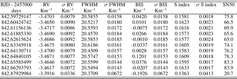
Table .1.Continued.
BJD - 2457000 RV σRV FWHM σFWHM BIS σBIS S index σS index SN50
days Km−1 Km−1 Km−1 Km−1 Km−1 Km−1
842.59729147 -3.4703 0.0079 20.5855 0.0158 0.0420 0.0158 0.1581 0.0018 75.8
842.60424742 -3.4650 0.0090 20.5217 0.0180 0.0101 0.0180 0.1623 0.0023 66.5
842.61156136 -3.4717 0.0086 20.5593 0.0172 -0.0075 0.0172 0.1616 0.0021 69.9
842.61885330 -3.4690 0.0092 20.4570 0.0184 0.0266 0.0184 0.1573 0.0023 65.6
842.62615624 -3.4686 0.0092 20.5853 0.0185 -0.0010 0.0185 0.1577 0.0024 65.0
842.63345918 -3.4675 0.0080 20.6186 0.0161 -0.0337 0.0161 0.1605 0.0019 74.1
842.64130711 -3.4700 0.0079 20.4509 0.0157 0.0028 0.0157 0.1583 0.0019 76.2
842.64840105 -3.4871 0.0077 20.5747 0.0153 0.1201 0.0153 0.1609 0.0018 78.3
842.65585499 -3.4646 0.0072 20.5599 0.0144 0.0376 0.0144 0.1595 0.0017 83.3
842.66293793 -3.4617 0.0072 20.5494 0.0143 -0.0207 0.0143 0.1633 0.0017 83.9