Effect of Orifice Introduction on the Pneumatic Separation of Spherical Particles

Effect of Ori

fi

ce Introduction on the Pneumatic Separation of Spherical Particles

Naohito Hayashi

and Tatsuya Oki

Research Institute for Environmental Management Technology, National Institute of Advanced Industrial Science and Technology (AIST), Tsukuba 305-8569, Japan

In order to recycle important rare metals (such as tantalum) in the print circuit boards of waste electronic equipment, the devices mustfirst be delaminated from the board. The devices are then separated into each device type such as capacitors, resistors, thermistors and so on. In this study, the effect of orifices on spherical particles was clarified through numerical simulations of airflow and air­solid multiphaseflow in a vertical single-column pneumatic separator. Airflow velocity profiles and particle trajectories were investigated for different numbers of orifices using spherical particles of identical size and different densities. By introducing multiple orifices, the eccentricity of the velocity profile in the vertical direction could be corrected. This eccentricity is caused by the presence of a mesh, which recovers heavy particles after they pass through the second orifice. When the distance between orifices ranged from 400 to 625 mm, it was expected that high-speed and high-efficiency separation between orifices would be possible. It implies that step-by-step separation could be conducted in a single separation column. However, under the calculation conditions of our study, the orifices did not affect the separation efficiency because this factor depends on the velocity profile around the feeding position. The separation rate was maximized when the orifices were separated by 625 mm.

[doi:10.2320/matertrans.M2013292]

(Received July 30, 2013; Accepted January 9, 2014; Published February 21, 2014)

Keywords: pneumatic separation, orifice, air­solid multiphaseflow, numerical simulation, discrete element method, printed circuit boards

1. Introduction

Printed circuit boards (PCBs) in electronic equipment include copper films, gold coats, and electronic devices containing specific precious and rare metals. For example, tantalum capacitors contain Ta, Mn, and Ag; ceramic capacitors contain Ba, Ni, Ag, and Pd; thermistors contain Ni, Pt, and Pd.1,2) _{Recycling systems are highly desired to} ensure a stable supply of these metals. However, because Cu and precious metals constitute the economic value of waste PCBs, recycling is largely restricted to recover by a copper smelting process. In this process, many rare metals such as Ta (selected by the Japanese government in 2012 as one offive rare metals to be recycled) are easily oxidized and distributed into slag. Retrieving rare metals from slag, however, is not economically viable.

Therefore, the recovery of main rare metals from waste PCBs must proceed in two steps: the delamination of electronic devices from waste PCBs and the separation of electronic devices containing specific rare metals. Delamina-tion of electronic devices is typically performed using a conventional impact crusher.3) _{The efficient separation of} specific device types from a mixture in electronic devices, on the other hand, has proven to be very difficult. If a high-accuracy separation method could be devised, objective metals could be recovered from the separated specific types of electronic devices by conventional hydrometallurgical processes.

Because Ta is present almost exclusively in tantalum capacitors in a PCB,4,5) it is preferential to recover these capacitors from mixtures of electronic devices delaminated from waste PCBs. One of the cited authors (Oki4,5)) has succeeded in recovering tantalum capacitors with high efficiency (72.4­92.2%). He used a vertical single-column pneumatic separator. In this process, the devices were set

vertically and the constituents were allowed to drop down by density, size, and shape of electronic devices. The separation rate increased when multiple throttles, also called orifices, were placed inside the column. The effect of these orifices, which reduced the inner diameter of the separation column over a short distance, was similar to that reported by Ito et al.6) _{In their experiments, the separation rate of Cu and} Al plate samples increased when a pneumatic separation technique was applied; in addition, the separation efficiency was retained with reduced airflow and was less affected by variations in airflow velocity. Oki et al.7) _{experimentally} demonstrated, however, that pneumatic separation produces little increase in either separation efficiency or rate in the case of spherical particles (unlike the rectangular or plate particles mentioned previously).

Therefore, in this study we attempted to clarify the relationship between the particle shape and effect of orifice introduction in a pneumatic separator by numerical simu-lations of air­solid multiphase flow combining the finite volume method (FVM) with the discrete element method (DEM). The separator was designed to segregate non-spherical particles such as electronic devices and metal plates. In this paper, we focused on spherical particles, for which it was experimentally demonstrated in a previous study that orifice introduction has little effect.7)_{We quantitatively} investigated the effects of orifices on the airflow velocity profiles and the trajectories of spherical particles of same diameter but different densities. In addition, we attempted to optimize the distance between orifices on the basis of separation efficiency and rate.

2. Methods

2.1 Simulation model

imental apparatus used; the calculation region is shown as a solid line. The dimensions of the cylindrical calculation region (diameter 84 mm; height 1625 mm) match those of a real pneumatic separator. The bottom and top of the column are designated as Inlet 1 and Outlet 1 of airflow, respectively. Thex- andz-axes are aligned with the horizontal and vertical directions, respectively. The y-axis points outward from the plane of the paper (front: positive, back: negative). The separation column was connected to a blower on the ground through a 90-degree elbow pipe in the experimental apparatus. The top of the column was approximately 2.5 m above the ground. Above the elbow, a straightening grating and a mesh for the recovery of heavy particles were set; the latter was tilted at 45°.

The airflow velocity profile at Inlet 1 (225 mm above the mesh center) was deflected along thexdirection by the mesh as described in more detail below. The feed point of the spherical model particles was 50 mm above Inlet 1. The initial velocity of the feed particles pointed in the negativex direction.

A specified number of orifices were inserted at equidistant intervals L (mm) along the column. The distance between Inlet 1 and the first orifice was set at 275 mm (height from the mesh center: h=500 mm). The inner diameter, height, and angle of each orifice were 74 mm, 50 mm, and 45°, respectively; these values were the same as the dimensions and orientation of the experimentally used orifice (Fig. 2).

The calculation region was divided into 320,000 control volumes for the airflow analysis; 20 in the radius direction, 64 in the cylindrical direction, and 500 in the axial direction. The time-averaged Reynolds equations were solved numeri-cally for each control volume. The standardk-¾ model was used as a turbulence model.

To analyze the behavior of the model particles in the column, DEM was applied. In DEM, the behavior of particles is simulated by equations of motion derived by considering all forces acting on the particles. The effects of contacting particles in the normal and tangential directions were modeled by the Voigt model,8)_{in which elastic springs and} viscous dashpots are connected in parallel. In addition, tangential friction between contacting particles was estimated by using a friction slider. FVM was coupled to DEM with respect to the drag force of airflow on the particles to analyze air­solid multiphase flow. Because the considered volume ratio of particles in the column was rather low (less than 0.1%), the airflow was not changed by the particleflow.

The restitution and friction coefficients between particles and between a particle and the wall in the DEM calculation had not been previously measured; we set them as 0.8 and 0.2, respectively. These values were assumed in previous papers on DEM simulation using plastic particles.9,10) Both the particles and the inner wall of the column were assumed to be made of epoxy resin in estimating the stiffness coefficients. From the Hertz elastic contact theory equa-tions11)_{with Poisson’s ratio 0.34 and the Young’s modulus} 3.1©109_N·m¹2_{, the normal and shear stiffness coefficients,}

KnandKs, were calculated as 8.3©107and 3.1©107N·m¹1, respectively. The time step, ¦t (s), is related to the normal stiffness coefficient as follows to ensure the stability of the numerical difference equations:

t2

ffiffiffiffiffiffiffi

m Kn

r

ð1Þ

Here, m is the mass of a particle. From this equation, we observe that ¦t increases when Kn decreases, resulting in shorter calculation times. According to Croweet al.,12)it is reasonable to assume that the particles possess small stiffness coefficients when the inter-particle contact phenomena exert little effect on particle behavior. Because the particle volume ratio in the calculation target was small and the airflow was thought to dominate particle behavior, the stiffness coefficient was set as 1/10,000 of that of epoxy resin on the basis of Fig. 1 Calculation region. Numbers are heights (in mm),)is the diameter

of the cylindrical separator, andLis the distance between orifices.

Φ74

45°

50 Φ84

preliminary calculations (normal stiffness coefficient, Kn: 8.3©103_N·m¹1_{; shear stiffness coefficient, K}

s: 3.1© 103_N·m¹1_{). Thus, the time step ¦t was set as 2.5©10}¹5_s from eq. (1). The physical properties used in the simulation model are summarized in Table 1.

2.2 Airflow analysis

A steady flow simulation was conducted in air at ambient temperature (density: 1.2 kg·m¹3, viscosity: 1.8© 10¹5m·s¹2) in the absence of particles. The average velocity of airflow introduced into the separation column was 12 m·s¹1, the same as the experiment.4,5) The experimental and calculated parameters were first used to estimate the airflow velocity profile at Inlet 1, which is shown as a horizontal solid line in Fig. 1.

The effect of the distance between orifices, L, was investigated in the steady flow simulation by varying the number of orifices from 0 to 5 and observing the resulting velocity profiles. Here,L was 1625 mm in the case without orifices and 1300, 625, 400, 287.5, and 220 mm in the cases with 1, 2, 3, 4, and 5 orifices, respectively.

2.3 Air­solid multiphase flow analysis

Terminal particle velocities provide a useful reference of airflow conditions inside the separation column in the pneumatic separation of solid particles. The terminal velocity, vt(m·s¹1), of a sphere of diameter,dp (m), can be obtained from the following equations by a numerical approach such as the Newton-Raphson method.12)

vt¼

ffiffiffiffiffiffiffiffiffiffiffiffiffiffiffiffiffiffiffiffiffiffiffiffiffiffiffiffi 4ðµpµgÞgdp

3µgCD

s

ð2Þ

CD¼ 24

Repð1þ0:15Rep

0:687_{Þ ð1<Re}

p<103Þ (2a)

CD¼0:44 ð103Rep<3105Þ (2b)

Rep¼dpvtµg

®g (2c)

Here, µp(kg·m¹3),µg(kg·m¹3),g (m·s¹2),CD(1),13)Rep(1) and ®g(m2·s¹1) are the particle density, air density, gravita-tional acceleration, drag coefficient, particle Reynolds number, and air viscosity, respectively.

SettingLto 275 mm in the calculation region in Fig. 1, the number of orifices was varied from 0 to 5 for four particle densities: 1500, 2500, 3500, and 4500 kg·m¹3_{. Spherical} particles of diameter 2 mm were assumed because the sizes of many electronic devices, such as ceramic capacitors, chip

resistors, jumper pins, and thermistors had been found to be mostly in 1­2 mm.4) _{These densities of spherical particles} were chosen so that the particles’ terminal velocities would be around the separation velocity of airflow. The separation velocity was set to 12 m·s¹1, the value used in the pneumatic separation experiments.4) The terminal velocities of the spherical particles of densities 1500, 2500, 3500, and 4500 kg·m¹3 were 8.2, 11, 13, and 15 m·s¹1, respectively. The shape and size of the particles were maintained constant to negate the effects caused by differences in shape and isolate the effects of orifice introduction. To inject the particles, four particles with different densities were aligned side by side parallel to theyaxis at the feeding point shown in Fig. 1 and released every 0.18 s. The initial particle velocity was set as¹1 m·s¹1_{in thex-axial direction, which is} the same as high-speed camera measurements of particles fed into the separator.

The velocity profile obtained by the airflow analysis for each number of orifices was set. The particle behavior attained a near-steady state 5 s after the start of feeding; therefore, the calculation was continued for 10 s to achieve an unambiguous steady state.

3. Results and Discussion

3.1 Airflow analysis

3.1.1 Velocity profile at Inlet 1

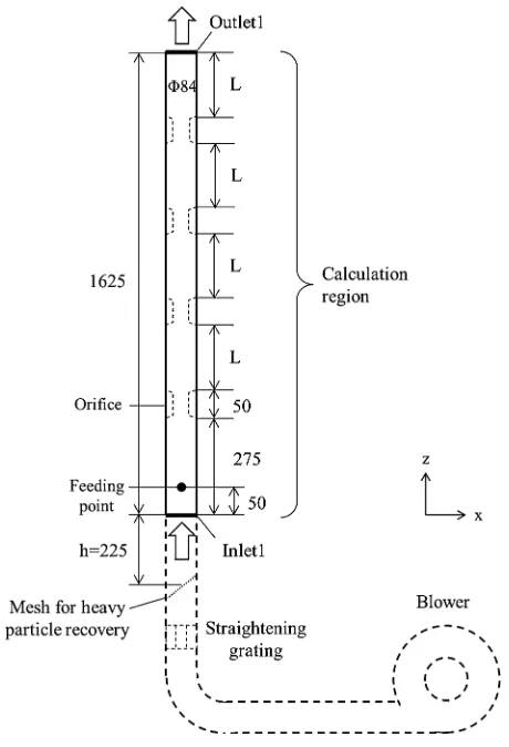
The airflow velocity in the experimental apparatus was measured to obtain the airflow velocity profile at Inlet 1 in Fig. 1. These measured values are plotted in Fig. 3, in which the origin is 225 mm above the mesh center (position of Inlet 1) and the x- andy-axes are defined as in Fig. 1. The average velocity was 12 m·s¹1_{. Airflow velocities to be} averaged were obtained by inserting a thermal anemometer (Kanomax Japan Inc., model 6332) for 10 s. Because large errors occurred near the inner wall of the column, the measurement range was restricted as¹20 to 20 along thex -and y-axes. Although the anemometer was non-directional, the obtained velocities were almost identical to those in the z-axial direction.

Because the mesh for heavy particle recovery was tilted 45° toward the lower part of the column, the velocity was higher in the negative region of the x-axis. The velocity profile was symmetric with respect to y=0 and convex Table 1 Physical properties for DEM simulation.

Restitution coefficient 0.8

Friction coefficient 0.2

Young’s modulus 3.1©109_N·m¹2

Poisson’s ratio 0.34

Normal stiffness coefficient,Kn 8.3©103N·m¹1 Shear stiffness coefficient,Ks 3.1©103N·m¹1

Time step,¦t 2.5©10¹5_s

downward along they-axis, because the airflow did not reach steady state at the measured positions.

The obtained velocity data were only along the x- and y -axes as shown in Fig. 3; there were no data between the x -and y-axes. Therefore, velocity data between the x- and y -axes should be estimated to appropriately set the velocity profile of Inlet 1 for the series of calculations involved in the multiphase flow simulation. Even though we measured velocities at small angle increments in the circumferential direction of the column (ª), an adequate interpolation method for the experimental data was necessary. The velocity profile at Inlet 1, therefore, was simulated by airflow analysis around a model mesh.

Uniform vertical airflow was introduced at 12 m·s¹1to the bottom of the separation column (Inlet 2) of diameter 84 mm and height 1000 mm, with no orifices. The center of the model mesh was 150 mm above the inlet. The calculation region and the model mesh are shown in Fig. 4. However, if a model mesh reflecting the too small wire diameter and open size of the real mesh (wire diameter and open size of 0.24 and 1 mm, respectively) was made, the control volumes for the flow calculation would become so fine that it would require an immense calculation time. Therefore, to use appropriate sizes of the control volumes for theflow calculation, a model mesh of wire diameter 1 mm and open size 2 mm was set in the column assuming that differences could be corrected by a coefficient.

Figure 5 shows the calculated velocity (absolute velocity) profile along thex- andy-axes 225 mm above the mesh center of Fig. 4, the experimental data from Fig. 3 included. The velocity (dashed line) approximates the experimental velocity along the y-axis, but the x-axial velocities deviate widely. The velocity was low in the positive region of thex-axis and high in the negative region, showing consistency with the experiment. These disagreements are attributable to the differences in wire diameter and open size between the

model and real meshes. The cross-sectional velocity profile obtained ath=225 mm is shown in Fig. 6. Here,“velocity” denotes absolute velocity but essentially shows the vertical velocity because the horizontal velocities are much smaller. The velocity profile is approximately symmetric with respect to thex-axis.

Next, the calculated velocities along thex- andy-axes were fitted to the experimental values through multiplication by a fitting coefficient. Appropriatefitting coefficients along thex -axis are selected as 0.7 and 1.1 for the positive and negative regions, respectively (dotted line in Fig. 5). The fitting coefficients were thought to depend on the modeling method of the mesh. The fitting was not applied to the y-axial velocities.

We supposed that the fitting coefficient changes linearly from 0.7 to 1 along the circumferential direction (ª) to set the velocity between the x- and y-axes; the fitting coefficient was divided into equal intervals according to the number of calculated values in the ª direction (64©1/4=16). Each linear increment was multiplied by the calculated velocity. The same treatment was applied to the x-negative and y -positive (range 1­1.1),x-negative andy-negative (range 1.1­ 1) and x-positive andy-negative (range 1­0.7) regions. The resulting velocity profile is assumed as the vertical velocity profile at Inlet 1 of Fig. 1 and is used in the simulation study (Fig. 7).

3.1.2 Effect of distance between orifices

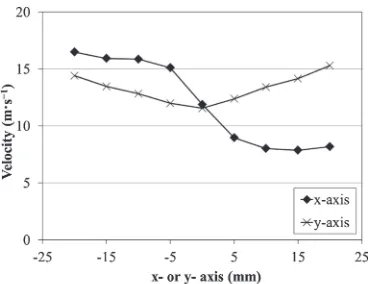
The steady flow simulations assumed that the vertical velocity profile (shown as a cross-section in Fig. 7) was identical to that at Inlet 1 of Fig. 1. The number of orifices was varied from 0 to 5. Figure 8 shows the vertical velocity profiles in the plane y=0. The distance between orifices, L, ranges from 1625 to 220 mm.

Although the average velocity in the separator was 12 m·s¹1, the velocity was significantly higher in the orifices, as evident in Fig. 8 (up to 20 m·s¹1in the red regions). The velocity was highest in the first orifice and was reduced at higher positions.

In the absence of orifices (Fig. 8(a)), particle separation was not achieved because the velocity eccentricity continued from the left side of Inlet 1 toward Outlet 1. In the presence of multiple orifices (Figs. 8(c)­8(f )), on the other hand, the 1000

Φ84

Inlet2 Outlet2

Model mesh

150 h=225 2

1

1 2

Fig. 4 Calculation region for obtaining the velocity profile at the Inlet 1 position (h=225);)is the diameter of the cylindrical separator, and all heights are in millimeters.

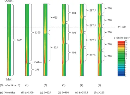
velocity eccentricity above the second orifice shifted to the column center for all values of L. The introduction of multiple orifices, therefore, corrected the horizontal velocity eccentricity which was caused at lower column positions. The cross-sectional velocity profiles at z=1100 mm above Inlet 1 are shown in Fig. 9 to quantitatively evaluate this correction effect. The numbers in the figures indicate the ratios of the distances between the column center and the centers of velocity profiles (eccentricity ratios). With an increasing number of orifices, the velocity profile center shifted gradually toward the column center and the eccentricity ratio decreased. As the number of orifices was increased further (from 2­4), the eccentricity ratio markedly

decreased (8.6%, to 6.3%, to 4.0%), revealing a compara-tively large horizontal velocity correction effect.

Both separation rate and efficiency should be increased by setting an appropriate distance between multiple introduced orifices. First, upward-dispersed particles will be transported quickly by the high-velocity airflow after passing through the orifice, improving the separation rate. Second, an ideal gravity concentration, in which gravity concentration is performed efficiently on the basis of a preliminary separation velocity, can be realized if airflow velocity is decreased and is uniform. We refer to this region as the “separation zone”. Ideally, the airflow velocity in the separation zone is identical to the preliminary separation velocity.

Fig. 7 Airflow velocity profile at Inlet 1 (h=225 mm) fitted to exper-imental data.

Velocities around the front of the second orifice in Fig. 8(c) (2 orifices) and around the third orifice in Fig. 8(d) (3 orifices) are close to the average velocity and are comparatively uniform; therefore, these regions were re-garded as the separation zones. Figure 10 shows the magnified velocity profiles around the separation zones in the cases of 2 and 3 orifices. The comparatively high velocity profiles shown in yellow, orange, and red (15­20 m·s¹1_{) at} the lower part of the separation zones appear to enhance the separation rate. In conclusion, when introducing multiple orifices and separating them byL=400­625 mm, high-speed

and high-efficiency separation should occur between the orifices. In other words, a step-by-step separation within a single separation column can be performed.

On the other hand, the comparatively high-velocity region shown in red, orange, and yellow continues from Inlet 1 to Outlet 1 in the cases of 4 and 5 orifices (Figs. 8(e) and 8(f )). In these cases, because the particles were exposed to airflow at higher-than-average velocities in the absence of a separation zone, particles of sufficiently high density had a higher probability of being recovered at Inlet 1, decreasing the separation efficiency. The volume ratios at which the vertical airflow velocity exceeded 13 m·s¹1were 38 and 40% in the cases of 4 and 5 orifices, respectively; therefore, we suggest that the number of upward-dispersed particles increases with increasing number of orifices in the absence of a separation zone.

3.2 Air­solid multiphase flow analysis 3.2.1 Effect on separation efficiency

In the air­solid multiphase flow simulation, the steady state of particle behavior was obtained assuming spherical particles of diameter 2 mm and densities 1500, 2500, 3500, and 4500 kg·m¹3.

Figure 11 shows the calculation result of the ratio of particles blown upward by airflow and recovered at Outlet 1. A 0% recovery ratio indicates that all particles had been dropped and recovered at Inlet 1. The horizontal axis shows the number of orifices. In 3.1.2, we deduced that an optimum distance between orifices of 400­625 mm, i.e., 2­3 orifices, yielded separation ratios close to 100%. Therefore, for spherical particles, the number of orifices apparently has a minimal effect on the separation efficiency. This result is the

(a) L = 645 mm (b) L = 400 mm

Fig. 10 Vertical airflow velocity profiles in the plane y=0 (around separation zone).

(a) No orifice (b) L = 1300 (c) L = 625

(d) L = 400 (e) L = 287.5 (f) L = 220

same as the experiments of Oki et al.7) and validates our analysis.

Particles tended to travel in a straight pass and collide with the left surface of the wall within the column. Shortly afterward, particles of densities 1500 and 2500 kg·m¹3(with terminal velocities less than the separation velocity of 12 m·s¹1) moved upward while those of densities 3500 and 4500 kg·m¹3_{(with terminal velocities exceeding the} separa-tion velocity) shifted downward. This tendency, observed for all numbers of orifices, is because the regions between Inlet 1 andz=250 mm developed the same velocity profiles regardless of the number of orifices (see Fig. 8). Within these regions, high-velocity regions (over 15 m·s¹1_{) developed at} the left side of Inlet 1, while the airflow in the remainder was close to average (11­13 m·s¹1_{). These airflow patterns} explain the abovementioned initial particle behavior. Sub-sequently, upward or downward velocity depended to some extent on particle density, but particles were essentially projected upward or dropped down to be discharged at Outlet 1 or Inlet 1. In this way, a very high separation efficiency was achieved. Few collisions occurred between particles. Because the airflow of the high-velocity region exceeded 15 m·s¹1_{above thefirst orifice and was magnified} with increasing numbers of orifices, particles of densities 3500 and 4500 kg·m¹3 _{were thought to project upward.} However, the vast majority of these particles reached no higher than the first orifice, with minimal effect on the separation ratio. A few particles of these densities, however, were blown beyond the first orifice and emerged at Inlet 1 owing to the near-ideal gravity concentration in the separation zone (see Fig. 10).

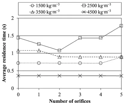
3.2.2 Effect on separation rate

Figure 12 shows the calculation result for the average residence time of particles of different densities. The residence time denotes the time between feeding and discharge from Outlet 1 or Inlet 1. Depending on the number of orifices, particles of density 2500 kg·m¹3_{were retained for} the longest duration in the column (residence time 1­1.8 s). Particles of densities 1500 and 2500 kg·m¹3_{, the terminal} velocities of which were very different from the 12 m·s¹1 separation velocity, were retained for shorter durations and

were rarely affected by the number of orifices. On the other hand, the residence times of particles of densities 3500 and 4500 kg·m¹3, with terminal velocities close to 12 m·s¹1, were extended. The 3500 kg·m¹3 particles were discharged most quickly when two orifices were introduced; the residence time in this case was 30% lower than in the case with no orifices. Therefore, for spherical particles under the simulated conditions, we infer that without decreasing the separation efficiency, the treatment is most effective when the number of orifices is two; i.e., when the distance Lbetween orifices is 625 mm.

Analyzing the particle behavior in the column, we found that particles of density 1500 kg·m¹3_{collided with the inside} wall two or three times, reducing the velocity along the x-direction to nearly zero. Consequently, these particles were projected directly upward. The particles of density 4500 kg·m¹3, on the other hand, collided once with the inside wall and settled, following a parabolic path to Inlet 1. We infer that the residence times of high- and low-density particles are short and independent of the number of orifices from these particle behaviors.

Particles of density 2500 kg·m¹3 moved upward at lower speeds than those of density 1500 kg·m¹3_{. The upward} velocity was increased by the larger high-velocity region as the number of orifices increased. Two orifices yielded the highest velocity. As the number of orifices increased further, the particles collided more frequently with the orifices. Consequently, the residence time was increased because particles striking certain parts of the orifices were reflected vertically downward. The column height was maintained constant in the simulations. However, the results indicated that a shorter column height with reduced orifice spacing would increase the upward velocity of light particles and decrease the frequency of orifice collisions. We will investigate the effect of column height in future studies.

Particles of density 3500 kg·m¹3were rarely blown beyond thefirst orifice (the exceptions are described in 3.2.1). These particles repeatedly shifted upward and downward over a short distance around the feeding position, and then tended to drop down and discharge from Inlet 1. In this case, the effect of the number of orifices was not clear.

Fig. 12 Effect of the number of orifices and particle densities on average residence time.

4. Conclusions

The effects of orifices on the airflow velocity profile and on particle behavior were investigated using a vertical single-column pneumatic separator developed for nonspherical particles. Airflow and air­solid multiphase flow simulations were conducted assuming identically-sized spherical particles of different densities while the number of orifices (and consequently, the distance between orifices) was varied. The results are summarized as follows:

(1) The horizontal airflow velocity profile in the separation column was eccentric owing to the mesh inserted for heavy particle recovery in the lower part of the column. In the absence of orifices, the velocity profile remained eccentric at distances exceeding 1 m. When multiple orifices were introduced, however, the velocity eccen-tricity was corrected beyond the second orifice. (2) When the distance between orifices was 400­625 mm,

we expected that high-speed and high-efficiency separation had been achieved and that step-by-step separation had been attained in a single separation column. The separation efficiency finally attained was almost 100%, regardless of the number of orifices and orifice spacing. This was attributed to the same velocity profiles in the regions between the column inlet and the first orifice (including the feeding point), from which we deduced the behavior of spherical particles. (3) Particles having terminal velocities vastly different

from the separation velocity exhibited a short average residence time, which was independent of the number

of orifices. Particles with terminal velocities close to the separation velocity stayed longer in the column. The residence time of particles was shortest when the orifice spacing was 625 mm; therefore, we regarded this spacing optimal in terms of separation rate. With a higher number of orifices, the particles were more likely to collide with the orifices, counteracting the enhanced upward flow induced by the orifices.

REFERENCES

1) T. Yumoto and T. Shiratori:J. MMIJ125(2009) 75­80.

2) T. Yumoto, T. Shiratori and T. Nakamura:J. MMIJ126(2010) 95­102. 3) S. Owada, C. Koga, S. Kageyama, C. Tokoro, T. Shiratori and T.

Yumoto:J. MMIJ128(2012) 626­632.

4) T. Oki: Proc. The 50th Annual Conf. of Metallurgists of CIM, ed. by S. R. Rao, C. Q. Jia, C. A. Pickels, S. Brienne and V. Ramachandran, (CIM ICM, Montreal, Canada, 2011) pp. 69­77.

5) T. Oki, Y. Naito, T. Kamiya, K. Kawakita and T. Shiratori: Proc. XXV Int. Mineral Processing Congress (IMPC), (IMPC, Brisbane, Australia, 2010) pp. 3839­3844.

6) S. Ito, J. Lee and S. Arai:Resour. Process.49(2002) 121­127. 7) T. Oki, H. Yotsumoto and N. Ishida: AIST Annual Report, (AIST,

Tokyo, 2005) p. 268.

8) P. A. Cundall and O. D. L. Strack:Geotechnique29(1979) 47­65. 9) P. A. Moysey and M. R. Thompson: Powder Technol. 153(2005)

95­107.

10) E. Simsek, F. Sudbrock, S. Wirtz and V. Scherer:Powder Technol.221 (2012) 144­154.

11) W. Goldsmith:Impact: The Theory and Physical Behavior of Colliding Solids, (Dover Publications, New York, 2001) pp. 162­170. 12) C. Crowe, M. Sommerfeld and Y. Tsuji: Multiphase Flows with