Distributed current control for multi three phase synchronous machines in fault conditions

Distributed Current Control for Multi-Three Phase

Synchronous Machines in Fault Conditions

A. Galassini, A. Costabeber, M. Degano, and C. Gerada, PEMC group, The University of Nottingham

A. Tessarolo and S. Castellan, Department of Engineering & Architecture, The University of Trieste

Abstract—Among challenges and requirements of on-going electrification process and future transportation systems there is demand for arrangements with both increased fault tolerance and reliability. Next aerospace, power-train and automotive systems exploiting new technologies are delving for new features and functionalities. Multi-three phase arrangements are one of these novel approaches where future implementation of aforementioned applications will benefit from. This paper presents and analyses distributed current control design for asymmetrical split-phase schemes composed by symmetrical three phase sections with even number of phases. The proposed design within thedq0reference frame in nominal, open and short circuit condition of one three-phase system is compared with the vector space decomposition technique and further validated by mean of Matlab/SimulinkR

simulations.

Index Terms—Multi-three phase machine, current control, fault tolerance

I. INTRODUCTION

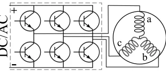
Electrification of future transportation systems is demanding for more reliability and fault tolerance than current fossil fuel solutions are able to guarantee. Nowadays, the multi-three phase machine concept is gaining popularity [1], [2] thanks to the repetition of a very well-known system: a two level voltage source converter controlling a three phase machine with a three phase set of windings (a,b,c) in Fig. 1. The repetition of this unit block (or module, or segment) establishes the multi-three phase machine concept in Fig. 2. The DC/AC converters are connected in parallel rather than in series. Indeed if wired in series, a fault in one converter would affect all the others.

The main advantage of the multi-three phase approach is the reuse of all the know-how regarding different control strategies, fault detection, fault isolation, and winding design for the unit block in Fig. 1. Many different solutions, strategies, and counter measures have been deployed along the years. Some solutions have taken advantages of additional switches or diodes introduction, whereas others simply re-configure the converter control strategy [3]–[5].

+

-a

b c

DC/AC

Fig. 1. Module made by one two level voltage source converter, one micro-controller (not shown), and one three phase sets of windings (a, b, c).

Fig. 2. Multi-three phase motor with paralleled distributed converters.

In this paper, the distributed current control in the dq0 reference frame of a quadruple-star synchronous motor in nominal and under faulty condition is presented and further validated using the so called vector space decomposition technique [6], [7] and Matlab SimulinkR _{simulations. In the}

next section, the machine model in dq0 reference frame [8], [9] is recalled in order to introduce the subsequent section. In Sec.III, the current control design in nominal condition within thedq0reference frame is detailed and further compared with the vector space decomposition algorithm. Sec.IV shows how to re-configure the healthy modules in both open and short cir-cuit condition avoiding instability issues. The reconfiguration is needed to guarantee, likewise stability margins, constant current control loops bandwidth and phase margin. In some applications, i.e. speed droop control of multi-three phase machine [10], constant current dynamics are needed. Before the conclusions in Sec.VI, the control design validation by means of Matlab/SimulinkR _{simulations is presented in Sec.V.}

II. MACHINE MODELLING

A. Modelling assumptions

The work presented in this paper is based on the assumption that stator inductances are constant. Therefore, it applies to electric machines with negligible saturation effects. In addition it is assumed that:

• all phases are geometrically identical;

• each phase is symmetrical around its magnetic axis;

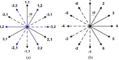
• the spatial displacement between two whatever phases is an integer multiple of the phase progressionα(Fig.3b);

• within the air-gap, only the fundamental component of magneto-motive force is considered.

B. Winding arrangement

Multi-three phase electrical motors are a particular group of split-phase winding machines. Defining m the number of phases per set of windings, in multi-three phase motorsm= 3

(phases a, b, and c in Fig.1). Therefore, definingNthe number of three phase systems (or unit block), the total number of phases is equal ton=N m. The motor modelled in this paper is composed by twelve phases, arranged in four three-phase sets of windings (m= 3, N = 4, n= 12). Considering the

(a) (b)

Fig. 3. TheW matrix maps the split-phase winding scheme with evenn in Fig.3a, denoted withabc, into the standard equivalent scheme with phase

progressionαin Fig.3b, denoted withstd.

case of an asymmetrical split-phase scheme composed of N

symmetrical m-phase sections with even number of phases

n=N m(Fig.3a), the permutation matrix

W(i,j)=

(_{1 ifi−trunc(}j−1

m )−2Nmod(j−1, m)−1 = 0 −1 if|i−trunc(j−_m1)−2Nmod(j−1, m)−1|=mN

0 otherwise

(1) maps the scheme in Fig.3a into the asymmetrical n-phase scheme (or standard equivalent scheme) with sequentially-distributed phases in Fig.3b (where trunc(x) is the largest integer less then or equal to x, mod(x, y) is the remainder on dividing xbyy, and i, j are row and column identifiers.) [9]. The phase progression in asymmetrical n-phase schemes is α =π/n. In Fig.3, for graphical simplicity’s sake n= 6

(m= 3,N = 2,α=π/6) but in this workn= 12. The stator inductance matrix of the standard (denoted with subscriptstd)

winding scheme in Fig. 3b has the structure shown in the followingnxn matrix:

Lstd=         

λ0 λ1 λ2 · · · −λ2 −λ1 λ1 λ0 λ1 · · · −λ3 −λ2 λ2 λ1 λ0 · · · −λ4 −λ3

..

. ... ... . .. ... ...

λ2 λ3 λ4 · · · −λ0 −λ1 λ1 λ2 λ3 · · · −λ1 −λ0

        

=WLabcWT

(2) The above relates the vectorφ_std of thenphase flux linkages to the vector istd of then phase currents (φstd =Lstdistd).

The Lstd matrix values will allow to verify the results

pre-sented in Sec.III and can be easily computed from the stator inductance matrix Labc by (1) and (2).

C. Analytical model in Park’s coordinates

Distributed current control is achieved within the rotor-attached orthogonaldq0 reference frame thanks to the Park’s transformation relating machine stator variables (denoted with subscript abc) to the dq0 ones (denoted with subscript dq). In distributed current control, there is one controller per three phase set and only the local three currents are provided as feedback. Since the machine is made by multiple three phase systems, the globalnxnPark’s transformation matrix is given by Eq. 3, where 03 is a 3x3 null matrix, and θ is the rotor

position.

T= 

 

T1 · · · 03

..

. . .. ...

03 · · · TN 

 

nxn

(3)

Th= r

2 3





cos[θ₋(h₋1)α] sin[θ₋(h₋1)α] 0

−sin[θ₋(h₋1)α] cos[θ₋(h₋1)α] 0

0 0 1









1 ₋1/2 ₋1/2

0 √3/2 ₋√3/2

1/√2 1/√2 1/√2



withh= 1..N

(4) The whole set of machine variables can be thus transformed into the dq0 reference frame. The machine voltage equation in the new coordinate system is:

vdq=Rdqidq+ωJLdqidq+Ldqd idq

dt +edq

withvdq= [vdq1· · ·vdqN]T,idq= [idq1· · ·idqN]T

andedq= [edq1· · ·edqN]T

wherevdqh= [vdh vqh v0h]T =Th[vah vbh vch]T

idqh= [idh iqh i0h]T =Th[iah ibh ich]T

edqh= [edh eqh e0h]T =Th[eah ebh ech]T =ωdφdqh/dt

(5) wherevdq, idq and edq are respectively voltage, current and

back electromotive force vectorsnx1.RdqandLdqare

respec-tively resistance and inductance matricesnxn,ω=dθ/dt, and

J= 

 

J1 _{· · ·} 03

..

. . .. ...

03 · · · JN 



; Jh=Th dTT

h

dθ = 



0 −1 0

1 0 0

0 0 0





(6) More precisely,Rabc=Rdq=rsI(nxn)wherersis the stator

phase resistance, whereas

Ldq= 

 

Ldq(1,1) · · · Ldq(1,N)

..

. . .. ...

Ldq(N,1) · · · Ldq(N,N) 

 

withLdq(i,j)=LTdq(j,i)=ThLabc(i,j)TTh =

= 3

2

Lmd 0 0

0 Lmq 0

0 0 0

!

+ Mi−j

−Xi−j 0

Xi−j Mi−j 0

0 0 Hi−j

!

where Lmd and Lmq are d, q magnetizing inductances.

Parameters Mk, Xk, Hk are the stator leakage inductances

expressed in the rotor dq0 reference frame. Their physical meaning is schematically shown in Fig. 4 (where i and j

are the stator set identifiers1..N) and they can be calculated with finite element analysis or analytic formulation [12], [13]. In particular, it can be seen that the mutual leakage

Fig. 4. Self and mutual inductances of stator dq0 circuits corresponding to the i-th and j-th stator three-phase set.M0is the self-leakage inductance.

inductance Xi−j couples the d-axis circuit corresponding to

the i-th set with the q-axis circuit corresponding to the j-th set of windings. It is worth to notice that d-qcross coupling depends on leakage fluxes alone and may occur only between

d andq circuits representing different stator sets (i.e. only if

i₆=j, henceX0−0= 0).

D. Leakage inductances

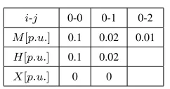
The stator leakage inductances in of the electric motor under investigation are reported in Table I. They are expressed in

p.u. using as base value of the impedance Vn/(√3InN),

whereVnandInare respectively nominal voltage and nominal

current. SinceX0−1= 0, there are nod-qinteractions between

TABLE I

STATOR LEAKAGE INDUCTANCES INdq0

i-j 0-0 0-1 0-2 M[p.u.] 0.1 0.02 0.01 H[p.u.] 0.1 0.02 X[p.u.] 0 0

different sets of windings. In the next section, for simplicity’s sake, whenever the current dynamic is the same in all the segments, only data regarding the first unit-block will be plotted. Actually, since in this particular case Lmd = Lmq,

only data regarding the q axis of the first module will be shown.

III. CURRENT CONTROL DESIGN IN NOMINAL CONDITIONS

In order to simplify the design of the distributed current con-trollers, this Section aims at finding a transfer function linking each element of the current vector only to the corresponding element of the voltage vector, with no other input acting as a disturbance. Unfortunately this is not possible by the analytical model indqcoordinates since the inductance matrixLdqis not

diagonal. In order to diagonalize the inductance matrix the vector space decomposition is used, as it will be explained in the following.

Since much faster than the rotor dynamic, the current control loop design based on the voltage stator equation (5) has been computed in blocked rotor condition. Therefore, the speed (ω) is zero, and (5) becomes:

vdq=Rdqidq+Ldqd idq

dt (8)

In state space model form, (8) becomes:

˙

xdq=Adqxdq+Bdqudq

ydq=Cxdq+Dudq

(9)

where xdq is the current state vector, udq is the applied

voltage input vector,ydq is the output current vector, Adq=

−L−_dq1Rdq, Bdq = L−_dq1, C and D are respectively identity

and null matrices nxn. Since Ldq is not diagonal, it is not

possible to get the decoupled transfer functions between the i-th input and j-th output with the following equation:

Gdq=C(sI−Adq)−1Bdq+D=Ydq/Udq (10)

whereIis identity matrix andsis the Laplace operator. Indeed

Gdqis not diagonal. In order to find the first harmonic inductor

value for designing the current controller in nominal condition, the matrix of inductances can be diagonalized thanks to the vector space decomposition (VSD) technique. The transforma-tion matrix Tvsd maps the orthonormal coordinatesdq0 into

the so calledvsdorthonormal space. Therefore

Lvsd =TTvsdLdqTvsd (11)

whereasRvsd=Rdq, sinceRdq is diagonal. The new input,

output and state space vectors in (12), respectivelyuvsd,yvsd

and xvsd, are the odd harmonic values of applied voltages,

output currents and state space values up to the 2ν + 1-th harmonic (withν =trunc((n−1)/2)), on both dandqaxes.

uvsd= [ud1 uq1 ud3 uq3 · · · ud(2ν+1) uq(2ν+1)]T yvsd= [yd1yq1 yd3 yq3 · · · yd(2ν+1)yq(2ν+1)]T xvsd= [xd1 xq1 xd3 xq3 · · · xd(2ν+1) xq(2ν+1)]T

(12)

Therefore, defining the new state space matrices Avsd =

−L−_vsd1Rvsd and Bvsd = L−vsd1, the decoupled transfer

func-tions have been computed in the vsd space thanks to the following equation:

Gvsd=C(sI−Avsd)−1Bvsd+D=Yvsd/Uvsd (13)

The matrixGvsdis diagonal and it describes the odd harmonic

dandqaxes. From this point, nominal, open and short circuit condition will be denoted respectively with subscriptN C,OC

andSC.

The Gvsd and Gdq transfer function nxn matrices link

input and output of two equivalent orthonormal spaces. Since the vsd space is related to the equivalent poly-phase winding

arrangement in Fig.3b, characterized by a symmetrical circu-lant structure inductance matrix like the one in (2), the Gvsd

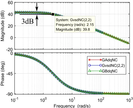
matrix is diagonal. In Fig.5 it is shown the equivalence of the following transfer functions: GAdqN C = Pnk=1GdqN C(k,2)

and GvsdN C(2,2). GAdqN C (in red asterisks) relates all the

-20 0 20 40 60

Magnitude (dB)

10-1 100 101 102 103

-90 -45 0

Phase (deg)

GAdqNC GvsdNC(2,2) GBdqNC

Frequency (rad/s) System: GvsdNC(2,2) Frequency (rad/s): 2.15 Magnitude (dB): 39.8

3dB

Fig. 5. Bode diagram comparing the transfer functions in bothvsdanddq state space models.

dq0 inputs with the q output current of the first set of windings xdq(2,1) in (9).GvsdN C(2,2) (in blue circles) relates

the first harmonic q input voltage with the first harmonic

q output current, xq1 in (12). In order to highlight that

the mutual leakage inductance X0−1 in Fig. 4 is zero, in

green triangles it is shown the transfer function GBdqN C =

PN

k=1GdqN C(3k−1,2) describing just the q output current

of the first set of windings taking into account only the q

input voltages (udq(2,1),udq(5,1),udq(8,1),udq(11,1)). The match

between GAdqN C and GBdqN C confirms that there are no

interactions among different axes of different sets of windings. The GvsdN C(2,2)transfer function pulsation in Fig.5 is

ωN C=rs/d1N C (14)

where d1N C is the first harmonic inductance in nominal

condition. Since rs can be easily measured and ωN C can

be extrapolated from Fig.5, d1N C computation is trivial.

However, in order to plot Fig.5,Gdq in (10) orTvsd in (11)

andGvsdin (13) must be numerically computed. Exactly the

same d1N C value and Lvsd diagonal matrix could have been

obtained analytically thanks to the vector space decomposition with the following equations [8], [9]:

dj = n X

k=1

λk−1cos[αj(k−1)] (15)

(where λk are the matrix values in (2)) keeping just the odd

elements up toj equal to2ν+ 1 like in the following:

Lvsd= 

         

d1 0 0 0 · · · 0 0

0 d1 0 0 · · · 0 0

0 0 d3 0 · · · 0 0

0 0 0 d3 · · · 0 0

..

. ... ... ... . .. 0 0

0 0 0 0 0 d2ν+1 0

0 0 0 0 0 0 d2ν+1



         

(16)

Since the first harmonic inductanced1describes the dominant

pole of the current dynamic on bothdandq axes, onced1 is

computed in nominal condition with one of the two presented methods,qanddcurrent proportional integral controllers (PI) in Fig.6 can be computed considering the plant in (17).

i

i

−

sKpN C+KiN C

s

e

sd1N C+rs

v

i

Fig. 6. Current control diagram within the synchronous reference frame without axes decoupling with first harmonic inductord1N C and the phase

resistorrs.KpN C andKiN Care the PI gains in nominal condition.

GvsdN C(2,2)= 1 sd1N C+rs

=

nN C X

k=1

GdqN C(k,2) (17)

In the next section open and short circuit conditions are detailed, and it will be shown that (15) is not valid for the short circuit condition.

IV. CURRENT CONTROL DESIGN IN FAULTY CONDITIONS

In a real case scenario, in a system like the one in Fig. 2, both on machine and inverter side, many different faults can occur. In this paper, for brevity, only the two following faulty conditions have been modelled: a) last set open (Fig. 7a), b) last set short circuited (Fig. 7b). In this work, it is assumed

DC

AC

(a) The last set is disconnected.

DC

AC

(b) The last set is in short circuit Fig. 7. Simulated faulty conditions.

that after a generic fault, the system is able to configure itself in one of these two configurations.

A. Open circuit

order in open circuit condition is equal tonOC =nN C−3 =

NOCm= 9, beingNOC = 3 instead of four. Therefore, the

new state space model indq0coordinates will be built without considering the last three rows and the last three columns of the state space model in nominal condition:

xdqOC=xdqN C(1:nOC,1), udqOC=udqN C(1:nOC,1)

ydqOC =ydqN C(1:nOC,1), LdqOC =LdqN C(1:nOC,1:nOC)

RdqOC=RdqN C(1:nOC,1:nOC)

CdqOC =I(nOC,nOC)DdqOC=0(nOC,nOC)

(18) Similarly to what has been done for the nominal

condi-25 30 35 40 45

Magnitude (dB)

100 ₁₀1

-90 -45 0

Phase (deg)

GvsdNC(2,2) GvsdOC(2,2) GAdqOC

Frequency (rad/s)

3dB

2.855rad/sec 2.855rad/sec

Fig. 8. Bode diagram comparing the dominant pole in nominal con-dition GvsdN C(2,2) versus the open circuit condition GAdqOC = PnOC

k=1 Gdq(k,2)=GvsdOC(2,2)

tion in the previous section, computing AdqOC,BdqOC, (10),

(11), (13) with the new variables defined in (18), the diago-nalised sub-state space model leads to a new transfer function

GvsdOC(2,2). In Fig.8, the bode diagrams of the dominant

transfer function in nominal (black line) and faulty conditions, both from vsd (yellow right triangles) and dq0 (magenta diamonds) state, have been reported. From the diagrams it is possible to appreciate the match between the two different coordinate systems and the difference between faulty and healthy state. The GvsdOC(2,2) differs from (17) only for the

inductance d1OC value that can be used for the design of

the current controller under open circuit condition. Like in nominal condition, the d1OC value can be computed by (15)

(withkranging from1tonOC) or it can be extrapolated from

Fig. 8.

B. Short circuit

The model describing the system in Fig.7b, with the last three phase set of windings in short circuit, is obtained imposing zero voltage on the fourth three phase set (vd4 = vq4 = v04 = 0V). The state space model order will be

the same of the one in nominal condition (nSC = nN C)

and for this reason (15) is not valid. Short circuit currents presence in the faulty set affects the current dynamic of healthy sets. According to the spatial disposition of the healthy three phase sets with respect to the faulty one (the fourth

-20 0 20 40 60

Magnitude (dB)

10-1 100 101 102 103 104

-90 -45 0

Phase (deg)

GvsdNC(2,2)

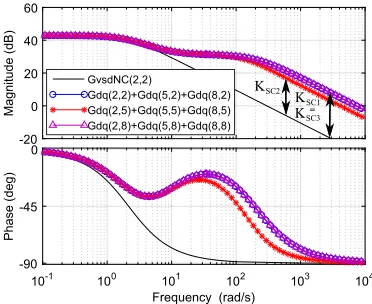
Gdq(2,2)+Gdq(5,2)+Gdq(8,2) Gdq(2,5)+Gdq(5,5)+Gdq(8,5) Gdq(2,8)+Gdq(5,8)+Gdq(8,8)

Frequency (rad/s) KSC2

KSC1

=

KSC3

Fig. 9. qoutput currents comparison between nominal and short circuited condition

one), current dynamics of the first and third three phase sets are identical, but they are different from that of the second three phase set. Transfer functions relating healthy q

input voltages (udq(2,1),udq(5,1),udq(8,1)) with healthyqoutput

currents (xdq(2,1),xdq(5,1),xdq(8,1)) are plotted in Fig.9. From

the diagrams it is possible to appreciate the difference between the second (red asterisks) set versus the first (blue circles) and the third one (magenta triangles). Since at high frequency all the sets of windings differ from nominal condition (black line), the proportional gains of the PI controllers must be updated in order to match the healthy system closed loop transfer function in Fig.6. It will be latter shown that determining the three high frequency magnitude differences between nominal and faulty condition transfer functions in Fig.9 (KSC1 =KSC3,

andKSC2) and updating the PIs as indicated in Table II, it is

possible to compensate the fourth set short circuit fault.

TABLE II

PIGAINS IN NOMINAL AND SHORT CIRCUIT CONDITIONS

set 1 2 3 4

KpNC KpNC KpNC KpNC KpNC

KpSC KpNC /KSC1 KpNC /KSC2 KpNC /KSC3

KiNC KiNC KiNC KiNC KiNC

KiSC KiNC /KSC1 KiNC /KSC2 KiNC /KSC3

V. SIMULATION RESULTS

The system has been simulated in all the conditions pre-sented above: nominal, open and short circuit condition. The

q currents iq1, iq2, iq3, iq4 of the four sets of windings are

respectively the2-nd,5-th,8-th and11-th element of the state space vector xdq in (9). The stator leakage inductances in

p.u. are reported in Table I, the magnetizing inductances and stator phase resistor are respectively Lmq =Lmd = 1.62H

and rs = 0.0072Ω. In nominal condition, the resulting first

harmonic inductance d1N C has been computed by (15) equal

(a) Current step in nominal condition (b) In OC the system with nominal PIs is stable. (c) In SC the PIs must be updated. Fig. 10. Current step in nominal condition and stability margins in faulty conditions.del2_=e−s1.5Ts _andc

f il=ωf2/(s2+ √

2ωfs+ω2f).

up with current bandwidth ωc = 600[rad/sec] and phase

margin ϕc= 60◦. In order to highlight how stability margins

are affected by faulty conditions, second order current filter and microprocessor actuation delay (e−s1.5Ts_{) have been}

in-troduced as shown by the block diagram of Fig.11. The delay has been set asTs= 2π/(25ωc)[sec]and the current filter

cut-off frequency as ωf = 66·103[rad/sec]. The PI parameters

i∗

i

−

P IN C

ei

e−s1.5Ts G_x i

ω2

f/(s2+

√

2ωfs+ω2f)

Fig. 11. Actuation delay and current filter have been introduced in order to highlight stability margin variations while keeping constant the PI gains in faulty conditions.

computation in nominal condition has led to KpN C = 2.12

andKiN C = 197.

A. Nominal condition

The output current in nominal condition of the control diagram in Fig.11 has been compared with the fouriq output

currents of a Simulink simulation with the four PI controllers regulating the whole dq0 machine model. In Fig.10a, it is possible to appreciate the match between the desired dynamic from the control diagram in Fig.11 and the four Simulink output currents with the same PI parametersKpN CandKiN C.

B. Stability margins in faulty conditions

In Figs.10b and 10c, stability margins of loop gain transfer functions in open and short circuit condition are shown. It is clear that without updating the controllers in open circuit the system is stable, whereas in short circuit the phase margin is very small.

C. Open circuit condition

In Fig.12a, the Simulink output currents with the last set of windings in open circuit condition (iq4 = 0) are reported.

In this situation the new first harmonic inductance d1OC has

been computed with (15) equal to0.0025Hand further verified

with (14) thanks to Fig.8. Since the PI parameters have not been updated, the resulting current dynamic do not match the desired one. In order to guarantee the nominal dynamic per-formance, the PI parameters must be re-calculated taking into account the new first harmonic inductanced1OC = 0.0025H

(KpOC= 1.59andKiOC = 149).

D. Short circuit condition

In Fig. 12b, system’s stability margins in SC with updated regulators are shown. Looking at Fig.10c, the phase margin improvement is clear. As detailed in Sec.IV-B in Table II, in short circuit condition the PI controllers must be divided by the KSCj factors which take into account the set

displace-ment within the stator. The calculations of the compensating factors in this particular case lead to the following values:

KSC2 = KSC8 = 23.13 and KSC5 = 14.07. The current

dynamic under short circuit condition with updated parameters is depicted in Fig.12c. Enhancement is highlighted comparing

iq1with nominal regulator underSCcondition (dash-dot line).

VI. CONCLUSION

This paper presents a distributed current control for multi-three phase synchronous machines with even number of phases under healthy and faulty conditions, e.g., one three-phase set of windings in open circuit, one set in short circuit. The plant for designing the current controller in healthy condition was numerically obtained diagonalising the state space model in the dq0 reference frame. The results were successfully compared against the ones analyticallyobtained thanks to the vector space decomposition. Furthermore, the same analysis and comparison was conducted with one three phase set of windings in open circuit condition. Finally, current control design in all the three conditions, respectively healthy, open, and short circuit were validated by mean of Matlab/SimulinkR _{simulations. Stability margin analysis}

(a)KpN C= 2.12,KiN C= 197 (b) Stability margins in SC, see Table II (c) See Table II

Fig. 12. Current step in OC (12a) with nominal regulators and in SC (12c) with updated ones. In Fig. (12b),P ISCh=KpSCh+KiSCh/s.

REFERENCES

[1] F. Barrero and M. J. Duran, “Recent advances in the design, modeling, and control of multiphase machines - part i,” IEEE Transactions on Industrial Electronics, vol. 63, no. 1, pp. 449–458, Jan 2016. [2] M. J. Duran and F. Barrero, “Recent advances in the design, modeling,

and control of multiphase machines - part ii,” IEEE Transactions on Industrial Electronics, vol. 63, no. 1, pp. 459–468, Jan 2016. [3] W. Zhang, D. Xu, P. N. Enjeti, H. Li, J. T. Hawke, and H. S.

Krish-namoorthy, “Survey on fault-tolerant techniques for power electronic converters,”IEEE Transactions on Power Electronics, vol. 29, no. 12, pp. 6319–6331, Dec 2014.

[4] B. Mirafzal, “Survey of fault-tolerance techniques for three-phase volt-age source inverters,” IEEE Transactions on Industrial Electronics, vol. 61, no. 10, pp. 5192–5202, Oct 2014.

[5] B. Welchko, T. Lipo, T. Jahns, and S. Schulz, “Fault tolerant three-phase ac motor drive topologies: a comparison of features, cost, and limitations,”IEEE Transactions on Power Electronics, vol. 19, no. 4, pp. 1108–1116, July 2004.

[6] A. Tessarolo, “On the modeling of poly-phase electric machines through vector-space decomposition: Theoretical considerations,” inPower En-gineering, Energy and Electrical Drives, 2009. POWERENG ’09. Inter-national Conference on, March 2009, pp. 519–523.

[7] E. Levi, R. Bojoi, F. Profumo, H. A. Toliyat, and S. Williamson, “Multiphase induction motor drives - a technology status review,”IET Electric Power Applications, vol. 1, no. 4, pp. 489–516, July 2007. [8] A. Tessarolo, L. Branz, and M. Bortolozzi, “Stator inductance matrix

diagonalization algorithms for different multi-phase winding schemes of round-rotor electric machines part i. theory,” inEUROCON 2015 -International Conference on Computer as a Tool (EUROCON), IEEE, Sept 2015, pp. 1–6.

[9] ——, “Stator inductance matrix diagonalization algorithms for different multi-phase winding schemes of round-rotor electric machines part ii. examples and validations,” inEUROCON 2015 - International Confer-ence on Computer as a Tool (EUROCON), IEEE, Sept 2015, pp. 1–6. [10] A. Galassini, A. Costabeber, C. Gerada, G. Buticchi, and D. Barater, “A

modular speed-drooped system for high reliability integrated modular motor drives,” IEEE Transactions on Industry Applications, vol. PP, no. 99, pp. 1–1, 2016.

[11] E. Klingshirn, “High phase order induction motors - part i-description and theoretical considerations,”IEEE Transactions on Power Apparatus and Systems,, vol. PAS-102, no. 1, pp. 47–53, Jan 1983.

[12] A. Tessarolo, M. Bortolozzi, and A. Contin, “Modeling of split-phase machines in park’s coordinates. part i: Theoretical foundations,” in

EUROCON, 2013 IEEE, July 2013, pp. 1308–1313.

[13] ——, “Modeling of split-phase machines in park’s coordinates. part ii: Equivalent circuit representation,” inEUROCON, 2013 IEEE, July 2013, pp. 1314–1319.

VII. BIOGRAPHIES

Alessandro Galassini(S’14) received the Master’s degree in Mechatronic Engineering in 2012 from the University of Modena and Reggio Emilia. He is currently a PhD student at the University of Nottingham. His research area is focused on integrated modular motor drives for multi-three phase machines.

Alessandro Costabeber(S’09M’13) received the Degree with honours in electronic engineering from the University of Padova, Padova, Italy, in 2008 and the Ph.D. degree from the same university in 2012, on energy efficient architectures and control techniques for the development of future residential microgrids. In 2014 he joined the PEMC group, Department of Electrical and Electronic Engineering, University of Nottingham, Nottingham, UK as Lecturer in Power Electronics. His current research interests include HVDC converters topologies, high power density converters for aerospace applications, control solutions and stability analysis of AC and DC microgrids, control and modelling of power converters, power electronics and control for distributed and renewable energy sources. Dr. Costabeber received the IEEE Joseph John Suozzi INTELEC Fellowship Award in Power Electronics in 2011

Michele Degano(M’15) received the Laurea degree in Electrical Engineering from the University of Trieste, Italy, in 2011 and the Ph.D. degree in Industrial Engineering from the University of Padova, Italy, in 2015. In 2015 he joined the Power Electronics, Machines and Control Research (PEMC) Group, University of Nottingham, U.K, as a Research Fellow. His main research interests are in the design and optimization of permanent magnet machines, reluctance and permanent-magnet-assisted synchronous reluctance motors through genetic optimization techniques, in applications ranging from small to large power. He is currently an assistent professor teaching advanced electrical machines at the University of Nottingham.

Chris Gerada(M’05) received the Ph.D. degree in numerical modeling of electrical machines from The University of Nottingham, Nottingham, U.K., in 2005. Since 2006, he has been the Project Manager of the GE Aviation Strategic Partnership. In 2008, he was appointed as a Lecturer in electrical machines; in 2011, as an Associate Professor; and in 2013, as a Professor at The University of Nottingham. His main research interests include the design and modeling of high-performance electric drives and machines. Prof. Gerada serves as an Associate Editor for the IEEE TRANSACTIONS ON INDUSTRY APPLICATIONS and is the Chair of the IEEE IES Electrical Machines Committee

Alberto Tessarolo(M06, SM15) received his Laurea and Ph.D. Degrees in Electrical Engineering from the University of Trieste, Italy, in 2000 and from the University of Padova, Italy, in 2011, respectively. Until 2006, he worked in the design and development of innovative motors and generators for high power applications with NIDEC-ASI (formerly Ansaldo Sistemi Industriali). Presently, he is with the Engineering and Architecture Department of the University of Trieste, Italy, where he teaches the course of Electric Machine Design. His main research interests are in the area of electric machine and drive modeling, design and analysis, a field in which he has authored more than 130 scientific papers. He acts as the principal investigator for various research projects in cooperation with leading electric machine manufacturers and final users, including the Italian Navy. He serves as an Editor for the IEEE TRANSACTIONS ON ENERGY CONVERSION and as an Associate Editor for the IEEE TRANSACTIONS ON INDUSTRY APPLICATIONS and the IET ELECTRIC POWER APPLICATIONS. He is a registered professional engineer in Italy.