(will be inserted by the editor)
SCIP-Jack – A solver for STP and variants with
parallelization extensions
Gerald Gamrath · Thorsten Koch ·
Stephen J. Maher · Daniel Rehfeldt ·
Yuji Shinano
the date of receipt and acceptance should be inserted later
Abstract The Steiner tree problem in graphs is a classical problem that com-monly arises in practical applications as one of many variants. While often a strong relationship between different Steiner tree problem variants can be observed, solution approaches employed so far have been prevalently problem-specific. In contrast, this paper introduces a general-purpose solver that can be used to solve both the classical Steiner tree problem and many of its vari-ants without modification. This versatility is achieved by transforming various problem variants into a general form and solving them by using a state-of-the-art MIP-framework. The result is a high-performance solver that can be employed in massively parallel environments and is capable of solving previ-ously unsolved instances.
1 Introduction
The Steiner tree problem in graphs (STP) is one of the classical N P-hard problems [1]. Given an undirected connected graphG= (V, E), costsc:E→
Q≥0 and a set T ⊆ V of terminals, the problem is to find a treeS ⊆G of minimum cost that spansT.
Practical applications of the STP can be found for instance in the design of fiber-optic networks [2]. However, it is more common that practical appli-cations are formulated as a particular variant of the STP [3, 4, 5, 6].
The announcement of the 11th DIMACS Challenge initiated our work with an investigation into the STP solver Jack-III, described in [7]. The model and code of Jack-III provided a base for the development of a general STP solver—being able to solve many of the problem variants. However,Jack-III is more than 15 years old. As such, many modern developments regarding STP solution methods and MIP solving techniques are not available. Our approach
to address this limitation of Jack-IIIincludes the combination of the model used in [7] with the start-of-the-art MIP-framework SCIP [8, 9]. Employing SCIPnaturally facilitated the incorporation of many algorithm developments from the past two decades and provided a platform for the development of new methods.
A major contribution of this paper is the development of a general Steiner tree problem solver. This achievement stands in contrast to the many problem-specific solvers observed within the literature. Furthermore,SCIPprovides a massively parallel MIP-framework that is employed with this general solver. Thereupon, bolstered by algorithmic improvements, the developed solver is able to solve several previously unsolved benchmark instances. Detailing the approach delineated above, the remainder of this paper will be structured as follows:
– Section 2 demonstrates the impact of transitioning from a simple, ad hoc created branch-and-cut code to the use of a full fledged, state-of-the-art MIP-framework.
– Section 3 shows how to employ the versatility of MIP models to not only solve a whole class of related problem variants, but—in combination with further algorithmic advances—be competitive with or even superior to problem-specific state-of-the-art solvers.
– Finally, in Section 4 the potential from using hundreds of CPU cores to solve a single problem is illustrated.
The results achieved in this paper demonstrate the value of revisiting topics after some time. In our case this occurred in two steps: First, prior to the DIMACS Challenge, with the developments delineated above, and second, after the completion of the Challenge, when further algorithmic methods were devised and implemented to considerably enhance the performance of SCIP-Jack. Further examples of revisiting research topics can be found in [10, 11].
In general, it can be stated that a branch-and-cut based Steiner tree solver has three major components. First, preprocessing is extremely important. Apart from some instances either specifically constructed or insightfully hand-picked to defy presolving techniques, such as the PUC [12] and I640 [13] test sets, preprocessing is often able to significantly reduce instances. Results pre-sented in the PhD theses of Polzin [14] and Daneshmand [15] report an average reduction in the number of edges of 78 %, with many instances being solved completely by presolving. In computational experiments performed for this paper, reduction rates of more than 90 % for some Steiner problem variants (e.g., for the maximum-weight connected subgraph problem) are obtained.
Finally, the core of the approach is constituted by the branch-and-cut procedure used to compute lower bounds and prove optimality. The results of [14] show that many STP instances can already be solved by reduction-and heuristic-based approaches [14]. However, the failure of the state-of-the-art solver described in [14] to solve a number of hard instances that defy preprocessing highlights the importance of strong branch-and-cut procedures.
2 From simple hand tailored to off-the-shelf state-of-the-art
The model employed in the solverSCIP-Jack uses theflow-balance directed cut formulation described in [7]. This formulation provides a tight linear pro-gramming (LP) relaxation. It is built upon the directed equivalent of the STP, theSteiner arborescence problem (SAP): Given a directed graphD= (V, A), a rootr∈V, costsc:A→Q≥0 and a setT ⊆V of terminals, a directed tree (VS, AS)⊆D of minimum cost is required such that for allt ∈ T, (VS, AS) contains exactly one directed path fromrtot. Each STP can be transformed to an SAP by replacing each edge with two anti-parallel arcs of the same cost and distinguishing an arbitrary terminal as the root. This procedure results in a one-to-one correspondence between the respective solution sets, see [16] for a proof.
An integer program for the SAP can be obtained by introducing a variable ya for each arc a ∈ A with the interpretation ya = 1 if a is in the Steiner arborescence, andya = 0 otherwise. These considerations set the stage for the following formulation:
Formulation 1 Flow Balance Directed Cut Formulation
mincTy (1)
y(δ+(W)) ≥ 1, for all W ⊂V, r∈W,(V \W)∩T 6=∅(2)
y(δ−(v))
= =
≤
0 ifv=r, 1 ifv∈T\r, 1 ifv∈N,
for allv∈V (3)
y(δ−(v)) ≤ y(δ+(v)), for allv∈N (4)
y(δ−(v)) ≥ ya, for alla∈δ+(v), v∈N (5)
0≤ya ≤ 1, for all a∈A (6)
ya ∈ {0,1}, for alla∈A (7)
whereN=V\T,δ+(X) :={(u, v)∈A|u∈X, v∈V\X},δ−(X) :=δ+(V\X) forX⊆V; i.e.,δ+(X) is the set of all arcs going out of, andδ−(X) the set of
all arcs going intoX.
Since the model potentially contains an exponential number of constraints a separation routine is employed. Violated constraints, are separated during the execution of the branch-and-cut algorithm.Jack-III employed this prob-lem formulation along with a model-specific branch-and-bound search. Strong branching [17] was used with a depth-first search node selection.
The implementation of SCIP-Jack is based on the academic MIP solver SCIP[8, 9]. Besides being one of the fastest non-commercial MIP solvers [18], SCIP is a general branch-and-cut framework. The plugin-based design of SCIP provides a simple method of extension to handle a variety of specific problem classes.
In the case of SCIP-Jack, the first plugins implemented were a reader
to read problem instances andproblem data to store the graph and build the model within SCIP. Within these plugins it was possible to re-use the read-ing methods and data structures of Jack-III. However, each of these had to be extended as part of the implementation in SCIP-Jack. The heart of the new implementation is aconstraint handler that checks solutions for feasibil-ity and separates any violated model constraints. Again, separation methods of the more than 15-year old code are re-used in SCIP-Jack, while SCIP provides a filtering of cuts to improve numerical stability and dynamic aging of the generated cuts. Additionally, the general-purpose separation methods that exist within SCIP are used, which include Gomory and mixed-integer rounding cuts.
Jack-IIIincludes many STP-specific preprocessing techniques, as described in [7]. However, forSCIP-Jack only the Degree-Test (DT) [19] method has been reused. All other tests were replaced by more efficient variants, which have emerged in the decade following the release of Jack-III, cf. [14]. More-over, after the DIMACS Challenge work on reduction techniques continued and various new reduction methods were developed for several of the Steiner problem variants described in this paper. They are a pivotal factor in the improved performance of SCIP-Jackas compared to its predecessor partici-pating in the Challenge—the main motivation behind the development of the new methods was to enhance SCIP-Jack [16]. Due to the large number of presolving techniques and their complexity it is not possible to provide in-dividual descriptions within the frame of this paper. The reader is referred to [16] for detailed information. The preprocessing techniques implemented in SCIP-Jackare listed in Table 2 according to the abbreviations used in [16]; the full names of the preprocessing techniques can be found in Section B of the appendix. Supplementary to the presolving techniques, a Steiner problem specific propagator is implemented that fixes edges during the branch-and-cut according to the same criteria used in the dual-ascent (DA) reduction method [13, 14].
branch-and-bound procedure, vertex branching selects a Steiner vertex to be rendered a terminal in one child node and excluded in the second child.
Determining such a Steiner vertex is achieved by means of the following criterion. Lety∈[0,1]Abe an LP solution at the current node during branch-and-cut. Select a vertexvi∈V \T to branch upon, such that
X a∈δ−(v
i)
ya−0.5
(8)
is minimal among all Steiner vertices.
The node selection is organized by SCIPand is performed with respect to a best estimate criterion—interleaved with best bound and depth-first search phases [21].
One dual and several primal STP-specific heuristics have been implemented in SCIP-Jack—the dual-ascent heuristic (DA), the repetitive shortest path heuristic (RSPH), in the form proposed in [22], an improvement heuristic (VQ) [23], the reduction-based heuristics prune (P) and ascend-and-prune (AP) [14], and a new recombination heuristic (RC).
The dual-ascent algorithm was introduced in [24]. It exhibits a time com-plexity of O(|E|min{|V||T|,|E|}), see [14], but is usually faster than this bound might suggest; efficient implementations can be found in [13] and [25]. InSCIP-Jackthe implementation of [25] is used. At termination, dual-ascent provides a dual solution to a reduced version of Formulation 1 that contains only the constraints (2) and (6). This solution involves directed paths along arcs of reduced cost 0 from the root to each other terminal. The heuristic is executed prior to the branch-and-cut procedure and includes all cuts corre-sponding to the dual solution found by DA. Due to strong duality, the objective value of the first LP solved during branch-and-cut corresponds to the objective value of the dual solution found by DA.
On the primal side,SCIP-Jackincludes the well-known repetitive shortest paths heuristic. Starting with a single vertex, the heuristic iteratively connects the current subtree to a nearest terminal by a shortest path. This procedure is reiterated until all terminals are spanned. The heuristic is implemented in Jack-III, but in its original form detailed by [26]. In SCIP-Jack an em-pirically faster version based on Dijkstra’s algorithm [22] is implemented. In addition to being used as an initial heuristic, the RSPH is also employed, with altered costs, during the branch-and-cut. Specifically, given an LP optimal solution y ∈ QA, the heuristic is called with the costs (1−y
a)·ca for all
a∈A. Thus, a stimulus for the heuristic to choose arcs contained in the LP
before and after the processing of a (branch-and-bound) node, after each cut loop and after each LP solving during a cut loop.
The improvement heuristic VQ is a combination of the three local search heuristics vertex insertion, key-path exchange, and key-vertex elimination as described in [23]. The basic idea of vertex insertion (denoted by V) is to connect further vertices to an existing Steiner tree in such a way that expensive edges can be removed. Key-vertices with respect to a treeS are either terminals or vertices of degree at least three in S. Correspondingly, a key-path is a path in S with a vertex at both endpoints, but without any intermediary key-vertices. A key-path exchange attempts to replace existing key-paths by others that are less costly. Similarly, for key-vertex elimination in each step a non-terminal key-vertex and all adjoining key-paths (except for the key-vertices at their respective ends) are extracted and an attempt is made to reconnect the disconnected subtrees at a lower cost. As in [23], the combination of key-path exchange and key-vertex elimination is denoted by Q. VQ is called for a newly found solution whenever the latter is among the five best known solutions.
The prune heuristic comes with a less customary approach obtained by building upon bound-based reductions introduced in [14] that were afterwards slightly improved in [16]. While for the original bound-based reductions an upper bound is provided by the weight of a given Steiner tree, in the prune heuristic the bound is reduced such that in each iteration a certain proportion of edges and vertices is eliminated. Thereupon, all exact reductions methods are executed on the reduced graph, motivated by the assumption that the (possibly inexact) eliminations performed by the bound-based method will allow for further (exact) reductions. To avoid infeasibility, a Steiner tree is initially computed by using RSPH and afterwards the elimination of any of its vertices by the bound-based method is being prohibited. WithinSCIP-Jack the heuristic is called whenever a new best solution has been found.
Another powerful heuristic approach is borne by the combination of the prune heuristic and dual-ascent: the ascend-and-prune [14] method. Ascend-and-prune is motivated by the assumption that certain similarities exist be-tween an optimal Steiner tree and the LP solution that is identified by the reduced costs provided by dual-ascent. Thereupon, the heuristic attempts to find an optimal solution on the graph constituted by the undirected edges corresponding to zero-reduced-cost paths from the root to all additional ter-minals. On this subgraph a solution is computed by first employing an (exact) reduction package and then using the prune heuristic. Within SCIP-Jack, ascend-and-prune is performed after each execution of dual-ascent, in partic-ular prior to the initiation of the branch-and-cut procedure.
The heart of RC is then-merging (n≥2) operation subsequently defined for a given solutionS0 to an STPP= (V, E, T, c):S0is merged with pseudo-randomly selectedn−1 solutionsS1, ..., Sn out ofL \ {S0}to form a new STP
˜
P consisting of all edges and vertices that are part of at least one of the n solutions. By applying the reduction techniques provided by SCIP-Jack to
˜
P, a reduced problem ˜P0 is obtained. Thereupon, a solution to ˜P0is computed
in several steps. First, it is observed that each edge ein ˜P0 corresponds to a set of ancestor edgesEe⊆E. Denoting the edges of a solutionS
ibyESigives
the definition:
α(e) = Pn
i=0|E
e∩E Si|
|Ee| .
Next, the cost of each edge e in ˜P0 is multiplied by a pseudo-randomized number that is anti-proportional to α(e) (i.e., the number increases as α(e) decreases). This edge cost multiplication approach is a more general variant of a procedure suggested in [27]. The latter approach recombines two solutions without employing reduction techniques. Using the new edge cost, RSPH is employed to obtain a solution ˜S0 to ˜P0. For the starting points of RSPH, ver-ticesviare used such thatPe∈δP˜0(vi)α(e) is maximized. Next, after retrieving
the original arc costs, VQ is applied on ˜S0. Finally, ˜S0 is retransformed to the original solution space.
The RC heuristic is clustered around then-merging operation: Given a new solutionS, in onerunconsecutively six 2-, two 3- and one 4–merge operations are performed. When a solution S0 is generated during an n-merging with a
smaller cost thanS, the solutionSis replaced byS0, which is attempted to be
added toL. Moreover, in this case then-merging is performed again in a new run that is started after the conclusion of the current run. The total number of runs is limited to ten. RC is called wheneverrnew solutions have been found compared to its last execution. Initially,ris set to 4 and modified throughout the solution process, settingr:= 0 if a solution has been improved during the execution of RC andr:= min{r+ 1,4}otherwise.
By the combination of the previously described heuristics the ability to gen-erate good primal solutions quickly is considerably improved, as compared to employing SCIP-Jack without Steiner problem specific heuristics. Further-more, this combination is able to eventually find optimal solutions to most problems.
2.1 Computational experiments
Several thousand instances of 15 Steiner tree problem variants were collected as part of the DIMACS Challenge. To show the performance of the developed general Steiner tree problem solver, computational experiments on ten variants of the STP will be presented.
14.04. A development version ofSCIP3.2.1 was used andSoPlex[28] version 2.2.1 was employed as the underlying LP solver. Moreover, the overall run time for each instance was limited by two hours. If an instance was not solved to optimality within the time limit, the gap is reported, which is defined as
|pb−db|
max{|pb|,|db|} for final primal bound (pb) and dual bound (db). The average
gap is obtained as an arithmetic mean. The averages of the number of nodes and the solving time are computed by taking the shifted geometric mean [21] with a shift of 10.0 and 1.0, respectively.
Prior to the discussion of the different STP variants solved bySCIP-Jack in the following section, the solver performance will be demonstrated on pure STP instances. To this end, six STP test sets have been selected for com-putational experiments. Five of them, X [7] E [29], I640 [13], PUC [12], and ALUE [7], are test sets from SteinLib. First, the three X instances include complete graphs with Euclidean distances corresponding to geographical loca-tions (in Berlin, Brazil, and worldwide). In contrast, the E and I640 test sets contain randomly generated instances. The (sparse) E test set has proved to be solvable within short time limits by state-of-the-art solvers [14]. However, the I640 set—whose instances were selected to defy preprocessing—contains several problems that have remained unsolved until today. Similarly, many un-solved instances still remain in the PUC test set, which contains artificially de-signed problems such as instances composed of combinations of odd wheels and odd circles. As opposed to the previous three test sets, the ALUE instances are not artificially designed, but derive from a VLSI application and contain grid graphs with rectangular holes. The final test set is vienna-i-simple [2], which contains real-world instances generated from telecommunication networks that have already been preprocessed by the Degree-Test described in [19].
A summary of the computational performance of SCIP-Jack on the five STP test sets is presented in Table 1. Each line in the table shows aggregated results for the test set specified in the first column. The second column, labeled #, lists the number of instances in the test set, the third column states how many of them were solved to optimality within the time limit. The average number of branch-and-bound nodesand the average runningtime in seconds of these instances are presented in the next two columns, named optimal. The last two columns, labeled timeout, show the average number of branch-and-bound nodes and the average gap for the remaining instances, i.e., all
Table 1: Computational results for STP instances
optimal timeout
test set # solved ∅nodes ∅time [s] ∅nodes ∅gap [%]
X 3 3 1.0 0.3 – –
E 20 20 1.4 1.0 – –
ALUE 15 12 1.7 12.4 1.0 1.7
I640 100 78 17.7 9.3 85.3 0.8
PUC 50 8 406.8 36.9 121.9 3.5
instances that hit the time limit. In the next section, similar tables will be presented for different STP variants. If all instances of a particular variant are solved to optimality within the time limit, thetimeout columns are omitted. Detailed instance-wise computational results of all experiments can be found in Appendix C.
The instances from the X test set is solved without any branching and in very short run times; even the largest instance, consisting of more than 200 000 edges, requires only one second. Similarly,SCIP-Jack solves the en-tire, mostly sparse, E test set to optimality within an average time of 1.0 seconds. The only instance requiring branching is e18, which also exhibits a run time much longer than any other of that test set, 104.5 seconds. The, similarly sparse, VLSI-derived ALUE instances are harder to solve for SCIP-Jack: three problems remain unsolved with gaps of 1.4, 1,5, and 2.3 percent, while the solved instances require an average run time of 12.4 seconds. For only three of the instances branching is performed, and none requires more than five nodes.
SCIP-Jack exhibits a distinctively disparate behavior on the I640 test set: While more than half of the instances are solved within a few seconds, 22 problems remain unsolved after two hours. As compared with the previous instances the number of branch-and-bound nodes is much higher—up to 4481. The PUC test set proves to be much more difficult for SCIP-Jack. This is unsurprising since more than half of the instances in this set still remain unsolved.SCIP-Jack only solves eight of 50 instances and none at the root node. More than half of the unsolved instance are still processing the root node when terminated. Finally, 80 percent of the vienna instances set are solved by SCIP-Jack within the time limit, with none of the remainder exhibiting an optimality gap of more than 0.01%. As compared to the PUC test set, the number of branch-and-bound nodes is much smaller and more than half of the instances can be solved in the root.
The results demonstrate an improvement of SCIP-Jack in two dimen-sions. First, compared to Jack-III, SCIP-Jack empirically yields signifi-cantly better results, as exemplified by the E test set. While Jack-III and SCIP-Jackboth manage to solve all instances in relatively short times, there is a large difference in the run times achieved by each. Jack-IIIneeds more than one second for all but one instance. The hardest instance,e18, requires more than 11 minutes. In contrast,SCIP-Jacksolves all but three instances in less than a second, with a maximum runtime (fore18) of about two min-utes. On average,SCIP-Jackis more than two orders of magnitude faster on the E test set thanJack-III.
The second dimension is seen when comparing the performance of the cur-rent version ofSCIP-Jackwith its predecessor participating in the DIMACS Challenge, cf. [30]. In particular, computational experiments demonstrate that the current version is significantly stronger. Taking the example of the I640 test set, one sees additional 13 instances being solved to optimality within two hours. Also, the run time for several instances (such as i640-043) is reduced by a factor of more than a hundred.
The improvement of the current version of SCIP-Jackas compared with the previous version that competed in the DIMACS Challenge can be put down to several major algorithmic improvements. First, the implementation of new or enhanced problem-specific preprocessing methods, such as the dual-ascent reductions [31]. Second, the implementation of the new heuristics dual-ascent, and, on the primal side, prune, ascend-and-prune, and an improved version of the recombination heuristic. Third, the implementation of a problem-specific propagator and branching rule.
However, while the current version ofSCIP-Jackproves to be competitive with the best exact results obtained at the DIMACS Challenge, it falls short of matching the fastest STP solver described in the literature [14, 31]. Apart from very easy instances, such as in X, and the hard PUC test set, for which SCIP-Jackyields comparable results, the solver described in [14] (which uses the commercial CPLEX 12.61) is more than an order of magnitude faster for most instances [31].
3 From single problem to class solver
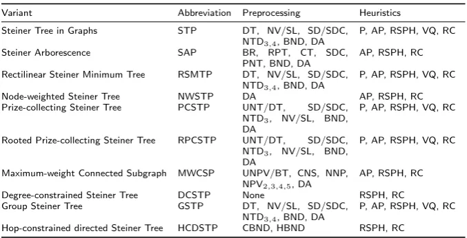
SCIP-Jack is developed as a general STP solver—being able to solve many problem variants. An overview of the problem variants solved bySCIP-Jack is given in Table 2. This table also presents the heuristics (see Section 2) and presolving techniques (see Table 14) that are applied to each of the problem variants. Specific transformation approaches have been employed in order to solve each variant by SCIP-Jack. Each of these transformations will be de-scribed in detail. Throughout this section the weights of an (undirected) edge eand an (directed) arcaare denoted byceandcarespectively and the weight of a vertexv bypv.
3.1 The Steiner arborescence problem
As SCIP-Jack transforms each Steiner tree problem to a Steiner arbores-cence problem (SAP), the branch-and-cut framework can be used for general SAPs with only minor modifications. Slightly modified forms of the RSPH, AP, and RC heuristics can also be used for SAP instances. However, due to the missing bi-direction with equal cost, the VQ heuristic cannot be applied.
Table 2: Problem variants solved by SCIP-Jack
Variant Abbreviation Preprocessing Heuristics
Steiner Tree in Graphs STP DT, NV/SL, SD/SDC, NTD3,4, BND, DA
P, AP, RSPH, VQ, RC
Steiner Arborescence SAP BR, RPT, CT, SDC,
PNT, BND, DA
AP, RSPH, RC
Rectilinear Steiner Minimum Tree RSMTP DT, NV/SL, SD/SDC, NTD3,4, BND, DA
P, AP, RSPH, VQ, RC
Node-weighted Steiner Tree NWSTP DA AP, RSPH, RC
Prize-collecting Steiner Tree PCSTP UNT/DT, SD/SDC, NTD3, NV/SL, BND, DA
P, AP, RSPH, VQ, RC
Rooted Prize-collecting Steiner Tree RPCSTP UNT/DT, SD/SDC, NTD3, NV/SL, BND, DA
P, AP, RSPH, VQ, RC
Maximum-weight Connected Subgraph MWCSP UNPV/BT, CNS, NNP, NPV2,3,4,5, DA
AP, RSPH, RC
Degree-constrained Steiner Tree DCSTP None RSPH, RC
Group Steiner Tree GSTP DT, NV/SL, SD/SDC,
NTD3,4, BND, DA
P, AP, RSPH, VQ, RC
Hop-constrained directed Steiner Tree HCDSTP CBND, HBND RSPH, RC
As to presolving techniques, besides DA, specific SAP reduction methods have been implemented—as described in [16].
[image:11.595.71.410.109.282.2]Computational results Computational experiments have been performed on two test sets of Steiner arborescence problems. These instances are derived from a genetic application [32]. The results are summarized in Table 3. The test sets contain small SAP instance, with the largest consisting of 602 nodes, 1716 edges and 86 terminals. Because of their size,SCIP-Jacksolves all instances within fractions of a second without requiring any branching. Furthermore, the reduction techniques eliminate more than 90 percent of the arcs on average.
Table 3: Computational results for SAP instances
test set # solved ∅nodes ∅time [s]
gene 10 10 1.0 0.2
gene2002 9 9 1.0 0.1
3.2 The rectilinear Steiner minimum tree problem
will be considered. The presented computational experiments include instances that derive from a cancer research application [3] and exhibit up to eight dimensions.
Hanan [37] reduced the RSMTP to theHanan-gridobtained by construct-ing vertical and horizontal lines through each given point of the RSMTP. It is proved in [37] that there is at least one optimal solution to an RSMTP that is a subgraph of the grid. Hence, the RSMTP can be reduced to an STP. Subsequently, this construction and its multi-dimensional generalization [38] is exploited in order to adapt the RSMTP to be solved bySCIP-Jack. Given
a d-dimensional, d∈ N\ {1}, RSMTP represented by a set ofn∈ N points
in Qd, the first step involves building a d-dimensional Hanan-grid. By using the resulting Hanan-grid an STP P = (V, E, T, c) can be constructed, which is handled equivalently to a usual STP problem bySCIP-Jack.
It certainly bears mentioning that this simple Hanan-grid based approach is not expected to be competitive with highly specialized solvers such as GeoSteiner [34] in the case d= 2. However, a motivation for the implemen-tation inSCIP-Jackis to address the obvious lack of solvers—specialized or general—that can provide solutions to RSMTP instances in dimensionsd≥3. Still, it is not practical to apply the grid transformation for large instances in high dimension, as the number of both vertices and edges increases exponen-tially with the dimension.
A variant of the RSMTP is the obstacle-avoiding rectilinear Steiner min-imum tree problem (OARSMTP). This problem requires that the minimum-length rectilinear tree does not pass through the interior of any specified axis-aligned rectangles, denoted asobstacles.SCIP-Jackis easily extended to solve the OARSMTP with a simple modification to the Hanan grid approach ap-plied to the RSMTP. This modification involves removing all vertices that are located in the interior of an obstacle together with their incident edges as well as all edges crossing an obstacle. There was no competition for this variant in the DIMACS Challenge and for the OARSMTP, unlike the RSMTP, optimal solutions to all instances submitted to the Challenge have already been pub-lished. WhileSCIP-Jackis capable of solving all instances submitted to the DIMACS Challenge, computational experiments for this problem variant have been omitted.
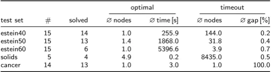
Computational results The experiments on the RSMTP involve solving five of the test sets submitted to the DIMACS Challenge. These test sets contain instances ranging from less than 10 to 10 000 points and from two to eight dimensions. Specifically, the test sets used in the presented experiments include the two-dimensional estein instances with up to 60 nodes, the solids test set with three-dimensional instances whose terminals are the vertices of the five platonic solids, and the real-world derived cancer instances in up to eight dimensions. Computational results are summarized in Table 4 with the detailed results listed in the appendix.
in-Table 4: Computational results for RSMTP instances
optimal timeout
test set # solved ∅nodes ∅time [s] ∅nodes ∅gap [%]
estein40 15 14 1.0 255.9 144.0 0.2
estein50 15 13 1.4 1868.0 31.8 0.4
estein60 15 6 1.0 5396.6 3.9 0.7
solids 5 4 4.9 0.2 8435.0 0.5
cancer 14 13 1.0 3.0 1.0 100.0
stances, the optimal solution was found at the root node. Also, none of the unsolved instances exhibits an optimality gap above 0.7 percent at the time limit. However, as the number of terminals increases, so does the run time and the number of unsolved instances: Only six of the estein60 instances can be solved within two hours, requiring more than twice as much time on aver-age than the estein50 problems. The optimality gap of the unsolved instances ranges from 0.1 to 1.6 percent. Only one of the estein60 instances requires branching—using 82 branch-and-bound nodes.
The results in Table 4 show the capabilities of SCIP-Jack to solve in-stances in three dimensions. Specifically, all but one of the solids inin-stances are solved to optimality. The unsolved instance, dodecahedron, is terminated after two hours with an optimality gap of 0.5 percent and 8435 branch-and-bound nodes. All other instances are solved in less than a second.
Finally, the cancer instances demonstrate the ability of SCIP-Jack to handle and solve RMST problems with up to eight dimensions. SCIP-Jack solves 13 of 14 instances to optimality at the root node. The remaining instance hits the memory limit after presolving—withSCIP-Jackcomputing a primal, but no dual bound. To the best of the authors’ knowledge,SCIP-Jackis the first solver to solve any of the cancer instances to optimality. Remarkably, more than half of the instances can be solved during preprocessing, including the cancer13 8D instance with more than a million arcs (in its transformed shape). Furthermore, only two of the solved instances require more than four seconds to achieve optimality. As compared to the previous version of SCIP-Jack competing in the DIMACS Challenge, cf. [30], the run times have considerably improved, mainly due to the enhanced reduction techniques (most notably DA), but also due to the new heuristics (most notably ascend-and-prune). For example, the cancer4 6D instance was not solved within 12 hours with the previous version, while the new version of SCIP-Jacknow proves optimality in less than 15 minutes.
3.3 The node-weighted Steiner tree problem
[image:13.595.105.376.111.183.2]while minimizing the weight summed over both vertices and edges spanned by the corresponding tree.
The NWSTP is formally stated by: Given an undirected graphG= (V, E), node costsp:V →Q≥0, edge costsc:E→Q≥0and a setT ⊆V of terminals, the objective is to find a treeS= (VS, ES) that spansT while minimizing
C(S) := X
e∈ES
ce+ X v∈VS
pv.
The NWSTP can be transformed to an SAP by substituting each edge by two anti-parallel arcs. Then, observing that in a tree there cannot be more than one arc going into the same vertex, the weight of each vertex is added to the weight of each of its incoming arcs.
Transformation 1 (NWSTP to SAP)
Given an NWSTPP = (V, E, T, c, p)construct an SAPP0= (V0, A0, T0, c0, r0)
as follows:
1. SetV0:=V,T0:=T,A0 :={(v, w)∈V0×V0:{v, w} ∈E}. 2. Definec0:A0→Q≥0 by c0a =c{v,w}+pw, for a= (v, w)∈A0.
3. Choose a rootr0∈T0 arbitrarily.
Lemma 1 (NWSTP to SAP) Let P = (V, E, T, c, p) be an NWSTP and
P0 = (V0, A0, T0, c0) an SAP obtained by applying Transformation 1 on P. Denote byS andS0 the set of solutions toP andP0 respectively. ThenS0 can be bijectively mapped onto S by applying
VS :={v∈V : v∈VS00} (9)
ES :={{v, w} ∈E: (v, w)∈AS00 or(w, v)∈A0S0} (10)
forS0= (VS00, A0S0)∈ S0 and it holds:
c0(A0S0) +pr0 =c(ES) +p(VS). (11)
The resulting SAP can be directly solved bySCIP-Jack. However, due to efficiency reasons only a subset of the heuristics and reduction techniques are employed, see Table 2.
Computational results Two NWSTP instances derived from a computational biology application are part of the DIMACS Challenge. The two instances differ drastically in their size. The first has more than 200 000 nodes—55 000 of them terminals—and almost 2.5 million edges, while the smaller instance comprises merely 386 nodes, 1477 edges, and 35 terminals.
employed to solve the NWSTP instance (in addition to the default prepro-cessing). After the application of the reduction techniques, the resulting graph contains 187 933 nodes and 986 703 edges. This equates to a 8.6 % and 60.4 % decrease in the number of nodes and edges respectively. SCIP-Jack fails to solve this instance to optimality, but it does achieve a nearly-optimal primal bound of 656 970.94 with an optimality gap of 0.0049%. The much smaller second instance is solved bySCIP-Jackat the root node within 0.1 seconds.
3.4 The prize-collecting Steiner tree problem
In contrast to the classical Steiner tree problem, the required tree for the
prize-collecting Steiner tree problem (PCSTP) needs only to span a (possibly empty) subset of the terminals. However, a non-negative penalty is charged for each terminal not contained in the tree. Hence, the objective is to find a tree of minimum weight, given by both the sum of its edge costs and the penalties of all terminals not spanned by the tree. A profound discussion on the PCSTP is given in [4] that details real-world applications and introduces a sophisticated specialized solver.
A formal definition of the problem is stated as: Given an undirected graph G= (V, E), edge-weightsc:E→Q≥0 and node-weightsp:V →Q≥0, a tree S= (VS, ES) in Gis required such that
P(S) := X
e∈ES
ce+ X v∈V\VS
pv (12)
is minimized.
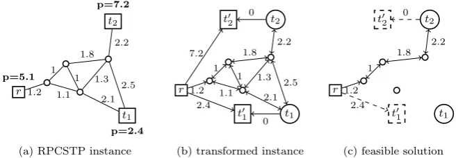
Prior to the discussion of the prize-collecting Steiner tree problem, a varia-tion is introduced, therooted prize-collecting Steiner tree problem (RPCSTP). The RPCSTP incorporates the additional condition that one distinguished
noder, denoted theroot, must be part of every feasible solution to the
prob-lem. It is assumed thatpr= 0. The RPCSTP can be transformed into an SAP as follows:
Transformation 2 (RPCSTP to SAP)
Given an RPCSTP P = (V, E, p, r)construct an SAPP0= (V0, A0, T0, c0, r0)
as follows:
1. SetV0 :=V,A0 :={(v, w) :{v, w} ∈E},r0 :=r andc0 :A0 →Q≥0 with c0a=c{v,w} fora= (v, w)∈A0.
2. Denote the set of allv∈V with pv>0 by T ={t1, ..., ts}. For each node ti ∈ T, a new node t0i and an arc a = (ti, t0i) with c0a = 0is added to V0
andE0 respectively.
3. Add arcs(r0, t0i)for eachi∈ {1, ..., s}, setting their respective weight topti.
r
p=5.1
t1 p=2.4
t2 p=7.2
1.2
2.1 2.5 2.2
1
1 1.3 1.8
1.1
(a) RPCSTP instance
r
t01
t02
t1
t2
1.2
2.1 2.5 2.2
1
1 1.3 1.8
1.1 2.4 7.2
0 0
(b) transformed instance
r
t01
t02
t1
t2
1.2
2.2
1 1.8
2.4 0
[image:16.595.76.406.104.218.2](c) feasible solution
Fig. 1: Illustration of a rooted prize-collecting Steiner tree instance with root r(left), the equivalent SAP problem obtained by Transformation 2 (middle), and a solution to the SAP instance with value 8.6 (right).
After Transformation 2, for each terminal t0i of the SAP P0 there are ex-actly two incoming arcs (ti, ti0) and (r0, t0). Thereupon, each solution S0 = (V0
S0, A0S0)∈P0 that containsti must also contain (ti, ti0), more succinctly:
∀i∈ {1, ..., s}:ti∈VS00 =⇒(ti, ti0)∈A0S0 (13)
Condition (13) is satisfied by all optimal solutions to P0 and each feasible solution can be easily modified to accomplish this, concomitantly improving its solution value. Transformation 2 is presented in [39], but without using condition (13). The latter gives rise to a one-to-one correspondence of the solution sets, stated in the following lemma.
Lemma 2 (RPCSTP to SAP) LetP0= (V0, A0, T0, c0)be an SAP obtained from an RPCSTPP = (V, E, c, p)by applying Transformation 2. Denote byS andS0the set of solutions toP andP0, satisfying condition (13), respectively.
P0 can be mapped bijectively ontoP by
VS :={v∈V : v∈VS00} (14)
ES :={{v, w} ∈E: (v, w)∈AS00 or(w, v)∈A0S0} (15)
forS0= (VS00, A0S0)∈ S0. The solution value is preserved.
Transformation 2 can be extended to cover the PCSTP by the inclusion of an artificial root node r0 and arcs (r0, ti) of cost 0. However, only one of these arcs can be part of a feasible solution. This requirement is enforced by the following constraint:
X a∈δ+(r0),c0
a=0
ya = 1. (16)
i is required to be part of the solution. This condition can be expressed by using the following set of constraints:
X a∈δ−(t
j)
ya+y(r0,t
i)≤1 i= 1, ..., s; j= 1, ..., i−1. (17)
An SAP that requires the conditions (13), (16) and (17) is referred to as root constrained Steiner arborescence problem (rcSAP). The constraints (16) and (17) can be incorporated into the cut-formulation (Formulation 1) without further alterations and each solution can be modified in order to meet condition (13). Although additional s(s2−1) constraints are introduced to fulfill (17), the solving time is considerably reduced by adding the constraints, as they exclude a plethora of symmetric solutions.
Transformation 3 (PCSTP to rcSAP)
Given an PCSTPP = (V, E, c, p)construct an rcSAPP0= (V0, A0, T0, c0, r0)
as follows:
1. Add a vertex v0 toV and setr:=v0.
2. Apply Transformation 2 to obtainP0= (V0, A0, T0, c0, r0). 3. Add arcsa= (r0, ti)with c0a:= 0 for each ti∈T.
4. Add constraints (16)and (17).
Lemma 3 (PCSTP to rcSAP) LetP= (V, E, c, p)be an PCSTP andP0= (V0, A0, T0, c0, r0) the corresponding rcSAP obtained by applying Transforma-tion 3. Denote byS andS0 the sets of solutions toP andP0 respectively. Each solution S0∈ S0 can be bijectively mapped to a solutionS∈ S defined by:
VS :={v∈V : v∈VS00} (18)
ES :={{v, w} ∈E: (v, w)∈AS00 or(w, v)∈A0S0}. (19)
The solution value is preserved.
For the PCSTP and RPCSTP a vast number of reduction techniques— described in [16]—are employed by SCIP-Jack, see Table 2. Furthermore, all heuristic used for the STP can be deployed, albeit with some alterations. For the RSPH in the case of a transformed PCSTP, i.e. an rcSAP, instead of commencing from different vertices, the starting point is always the (artificial) root. In each run all arcs between the root and non-terminals (denoted by (r0, t) in Transformation 3) are temporarily removed, except for one. A tree is then computed on this new graph, by using the same process as the original constructive heuristic. Instead of starting from a new terminal as done by customary RSPH, a different arc (r0, t) is chosen to remain in the graph.
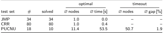
Table 5: Computational results for PCSTP instances
optimal timeout
test set # solved ∅nodes ∅time [s] ∅nodes ∅gap [%]
JMP 34 34 1.0 0.0 – –
CRR 80 80 1.0 0.4 – –
PUCNU 18 10 11.4 53.5 50.7 1.9
Computational results Table 5 shows aggregated results for three of the PC-STP test sets provided for the DIMACS Challenge. All but two JMP instances are solved during preprocessing in at most 0.1 seconds. The remaining prob-lems require no more than 0.2 seconds. Similarly, reduction techniques alone can solve 72 of the 80 CRR instances. However, the hardest (and considerably larger) instances take comparably longer—up to 3.7 seconds—to be solved to optimality. The third test set, PUCNU, is derived from the PUC test set for the STP.SCIP-Jackis already unable to solve many of the original instances and the PCSTP versions also prove to be hard. However, ten of the instances are solved to optimality, with only four instances requiring branching. The remaining eight instances terminate with optimality gaps in the range 1.0 % to 2.8 %.
Comparing the above results with those obtained by the previous version of SCIP-Jack, a significant improvement is observed. Specifically, the JMP and CRR instances can be solved more than 10 times faster on average, with the longest single run time of the previous version being almost 1000 seconds. This is compared to 3.7 seconds for the current version of SCIP-Jack. Moreover, three additional PUCNU instances can be solved within the time limit. A notable result is thatSCIP-Jacknow exhibits a better performance for 10 of the 12 JMP, CRR and PUCNU instances that were part of the exact DIMACS competition than any other participating solver at the time of the competition. The improved performance of SCIP-Jack can be traced to the vastly stronger new reduction techniques. However, it is also due to the new heuristics P and AP, and the general improvements of SCIP-Jack, such as the new propagator and the dual-ascent algorithm, which allows the start the branch-and-cut with a strong lower bound.
Table 6: Computational results for RPCSTP instances
optimal test set # solved ∅nodes ∅time [s]
cologne1 14 14 1.0 0.2
cologne2 15 15 1.0 0.6
[image:18.595.139.344.544.585.2]category of the RPCTSP, the current version requires significantly less time to solve the Challenge instances—being on average more than a factor of 25 faster for the cologne1 test set and more than a factor of 75 for the cologne2 set. This improvement is the result of the vastly improved preprocessing techniques, which alone manage to solve all cologne1 and cologne2 instances to optimality.
3.5 The maximum-weight connected subgraph problem
At first glance, the maximum-weight connected subgraph problem (MWCSP) bears little resemblance to the Steiner problems introduced so far: Given an undirected graph (V, E) with (possibly negative) node weightsp, the objective is to find a tree that maximizes the sum of its node weights. However, it is possible to transform this problem into a prize-collecting Steiner tree problem. One transformation is given in [5]. In this paper, an alternative transformation is presented that leads to a significant reduction in the number of terminals for the resulting PCSTP.
In the following it is assumed that at least one vertex is assigned a negative cost and at least one vertex is assigned a positive cost. Without this assumption the problem becomes trivial to solve.
Transformation 4 (MWCSP to rcSAP)
LetP = (V, E, p)be an MWCSP, construct an rcSAPP00= (V00, A00, T00, c00, r00):
1. SetV0:=V,A0 :={(v, w) :{v, w} ∈E}. 2. c0:A0→Q≥0 such that for a= (v, w)∈A0:
c0a=
−pw,ifpw<0 0, otherwise
3. p0:V0→Q≥0 such that forv∈V0:
p0(v) =
pv,if pv>0 0, otherwise
4. Perform Transformation 3 to (V0, A0, c0, p0), but in step 2 instead of con-structing a new arc set, A0 is being used. The resulting rcSAP gives us
P00= (V00, A00, T00, c00, r00).
Lemma 4 (MWCSP to rcSAP) Let P = (V, E, p) be an MWCSP and
P00 = (V00, A00, T00, c00, r00) an rcSAP obtained from P by Transformation 4. Then each solution S00 toP00 can be bijectively mapped to a solution S toP. The latter is obtained by:
VS :={v∈V : v∈VS0000} (20)
ES :={{v, w} ∈E: (v, w)∈AS0000 or(w, v)∈A00S00} (21)
Furthermore, for the objective value C(S) of S and the objective value
C00(S00)of S00 the following equality holds:
C(S) = X
v∈V:pv>0
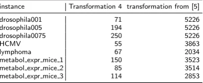
Table 7: Number of terminals after transformation for test set ACTMOD
instance Transformation 4 transformation from [5]
drosophila001 71 5226
drosophila005 194 5226
drosophila0075 250 5226
HCMV 55 3863
lymphoma 67 2034
metabol expr mice 1 150 3523
metabol expr mice 2 85 3514
metabol expr mice 3 114 2853
Since most of the vertex weights are non-positive for all real-world DI-MACS instances, Transformation 4 results in problems with significantly less terminals compared to the transformation described in [5]. The differences in the number of terminals resulting from the two transformations are pre-sented in Table 7. Even if the number of positive weight vertices is high in the original problem, after presolving it is typically much smaller, since adjacent non-negative vertices can be contracted [16].
For the MWCSP the computational settings of SCIP-Jackare similar to those of the (R)PCSTP. However, the VQ heuristic is not enabled since it cannot easily be adapted to handle anti-parallel arcs of different weight.
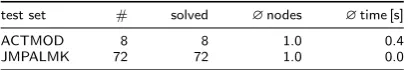
Computational results Computational experiments have been performed on the two MWCSP test sets that were part of the DIMACS Challenge. The first is the real-world derived ACTMOD test set (which contains eight instances), and second is the artificially created JMPALMK set (which contains 72 instances). The results, illustrated in Table 8, demonstrate the ability of SCIP-Jack to effectively handle real-world MWCSP instances of up to 93 000 edges in very short time: All eight instances can be solved within 1.4 seconds, in an average of less than half a second. The speedup of SCIP-Jack as compared to its DIMACS Challenge predecessor is impressive, ranging from a factor of ten to more than 4000. Furthermore, each instance is solved at least four times faster than by any solver during the DIMACS competition. A salient example is the drosophila001 instance which requires only 0.8 seconds withSCIP-Jack, but at least 21.6 seconds with any of the participating solvers at the time of the DIMACS competition. The drastically reduced run time ofSCIP-Jackis mainly due to new reduction techniques, but also the dual-ascent algorithm is a notable factor.
The results on the JMPALMK test set once again bespeak the strength of reduction techniques implemented inSCIP-Jack. All instances are solved during presolving, in an average of less than 0.1 seconds.
Table 8: Computational results for MWCSP instances
test set # solved ∅nodes ∅time [s]
ACTMOD 8 8 1.0 0.4
JMPALMK 72 72 1.0 0.0
3.6 The degree-constrained Steiner tree problem
Thedegree-constrained Steiner tree problem (DCSTP) is an STP with addi-tional degree constraints on the vertices, described by a function b:V →N. The objective is to find a minimum cost Steiner tree S = (VS, ES) such that
δS(v) ≤ b(v) is satisfied for all v ∈ VS. A comprehensive discussion of the
DCSTP, including its applications in biology, can be found in [6].
The implementation in SCIP-Jack to solve the DCSTP involves the ex-tension of Formulation 1 by an additional (linear) degree constraint for each vertex. Since the degree restriction does not comply with any reduction tech-niques of SCIP-Jack, problem-specific preprocessing has not been performed on these instances. Only the constructive heuristic is used, albeit in a modi-fied form. The implemented constructive heuristic performs the following two checks while choosing a new (shortest) path to be added to the current tree. First, whether attaching this path would violate any degree constraints. Sec-ond, whether after having added this path at least one additional edge could be added (or all terminals are spanned). If no such path can be found, a vertex of the tree is pseudo randomly chosen that allows to add at least one adjacent edge. Next, such an edge leading to a vertex of high degree and being of small cost is chosen.
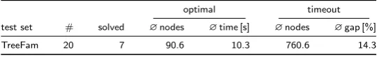
Computational results Computational experiments are performed on the 20 instances in the TreeFam test set of the DIMACS Challenge with a time limit of two hours. All instances come with degree bounds of at most 3 and their underlying graphs are complete.
The results from computational experiments on these instances are illus-trated in Table 9.SCIP-Jackfinds the optimal solution to five instances and proves the infeasibility of another two. The remaining 13 instances cannot be solved bySCIP-Jack within the time limit. The gap is reduced to less than or equal to one percent for seven of these instances. However, the gaps of the remaining six instances range from 4.5 to as much as 55.0 percent.
Similar to the preceding variants, the current version ofSCIP-Jack demon-strates improved performance over the previous version at the DIMACS com-petition. In particular, the insatisfiability of two instances can now be proven and both the run time for the solved instances and the gap for the remainder are significantly reduced: by a factor of more than 10 and by a factor of up to 100, respectively. This results in a reduction of the average gap (one of the criteria in the DIMACS Challenge) from 37.4 at the time of the competi-tion to 9.3 with the latestSCIP-Jack version. Note that the winner of this category reached an average gap of 19.1 in the competition. The improved solving behavior of SCIP-Jackon the DCSTP can be attributed to general enhancements such as the new propagator, see Section 2.
Table 9: Computational results for DCSTP instances
optimal timeout
test set # solved ∅nodes ∅time [s] ∅nodes ∅gap [%]
TreeFam 20 7 90.6 10.3 760.6 14.3
3.7 The group Steiner tree problem
Thegroup Steiner tree problem(GSTP) is another generalization of the Steiner tree problem that originates from VLSI design [20]. For the GSTP the concept of terminals as a set of vertices to be interconnected is extended to a set of vertex groups: Given an undirected graphG= (V, E), edge costsc:E→Q≥0 and a series of vertex subsets T1, ..., Ts ⊆ V, s ∈ N, a minimum cost tree spanning at least one vertex of each subset is required. By interpreting each terminaltas a subset{t}, every STP can be considered as a GSTP, the latter likewise beingN P-hard. On the other hand, it is possible to transform each GSTP instance (V, E, T1, .., Ts, c) to an STP by using the following scheme:
Transformation 5 (GSTP to STP)
Given an GSTPP = (V, E, T1, ...Ts, c)construct an STP P0 = (V0, E0, T0, c0)
as follows:
1. SetV0:=V,E0 :=E,T0=∅,c0:=c,K:=P
e∈Ece+ 1.
2. Fori= 1, ..., s add a new nodet0i toV0 andT0 and for all vj ∈Ti add an
edge e={t0i, vj}, withc0e:=K.
Let (V, E, T1, ...Ts, c) be a GSTP andP0= (V0, A0, T0, c0) an STP obtained by applying Transformation 5 onP. A solutionS0 to P0 can then be reduced to a solutionStoP by deleting all vertices and edges ofS not in (V, E). The GSTPP can in this way be solved on the STPP0 as shown in [20] and [40].
the time of publishing. In the case ofSCIP-Jack, to solve a GSTP, Transfor-mation 5 is applied and the resulting problem is treated as a customary STP that is solved without any alteration. An alternative approach would be to employ GSTP-specific heuristics or reduction techniques [42].
Computational results Computational experiments were performed on two test sets of unpublished group Steiner tree instances derived from a real-world wire routing problem. The results from these experiments are presented in Table 10. SCIP-Jack solves all but two of the first test set, with run times ranging from 3.3 to 563 seconds. Four of the instances solved to optimality only require a single node, with the remaining instances solved in 219 and 61 nodes, respectively. The two unsolved instances gstp34f2 and gstp39f2 exhibit optimality gaps of 2.7 % and 5.1 % respectively. The same performance is not observed for the second test set. None of the instances, are solved within the time limit and the optimality gaps range from 0.9 % to 7.8 %.
Table 10: Computational results for GSTP instances
optimal timeout
test set # solved ∅nodes ∅time [s] ∅nodes ∅gap [%]
GSTP1 8 6 14.9 25.0 355.9 3.9
GSTP2 10 0 – – 48.6 3.2
3.8 The hop-constrained directed Steiner tree problem
Thehop-constrained directed Steiner tree problem (HCDSTP) searches for an SAP with the additional constraint that the number of selected arcs must not exceed a predetermined bound, called hop limit. The cut formulation (For-mulation 1) used by SCIP-Jack is simply extended to cover this variation by adding one extra linear inequality bounding the sum of all binary arc vari-ables. It should be noted that in the literature the term ”hop-constrained Steiner tree” often refers to a problem for which the number of arcs in the path from the root to any terminal within a feasible solution is limited by a predefined bound [43], which differs from the definition used in this paper.
The hop limit brings significant ramifications for the preprocessing and heuristics approaches in its wake. Customarily, many presolving techniques for Steiner tree problems remove or include edges from the graph if a less costly path can be found, regardless whether this procedure leads to a solution with more edges. For the HCDSTP such techniques can therefore produce infeasibility. However, a number of HCDSTP-specific bound-based reduction techniques can be applied, as described in [16].
any identified solution may not be feasible. Therefore, a simple variation of the constructive heuristic is used for the HCDSTP: Each arc a, having orig-inal costs ca, is assigned the new cost c0a := 1 +λcmaxca , with λ ∈ Q+ and
cmax:= maxa∈Aca. Initiallyλis set to 3 but its value is decreased or increased after each iteration of the constructive heuristic, depending on whether the last computed solution exceeds or is below the hop limit, respectively. This modifi-cation toλis performed relative to the deviation of the number of edges from the hop limit.
Computational results Three different test sets, consisting of the gr12, gr14 and gr16 instances, are used for the computational experiments. All three test sets were used in the evaluation of the DIMACS Challenge. SCIP-Jack is able to solve all gr12 instances at the root node in less than 100 seconds. The performance worsens for the gr14 test set, with 12 of 21 instances being solved to optimality within the time limit. The unsolved instances terminate with optimality gaps ranging from 2.4 % to 17.9 %, after 8.8 nodes on average. Similarly, the optimally solved instances require—with 433.9 seconds—much more time than the previous problems (in gr12).
Table 11: Computational results for HCDSTP instances
optimal timeout
test set # solved ∅nodes ∅time [s] ∅nodes ∅gap [%]
gr12 19 19 1.0 4.0 – –
gr14 21 12 6.2 396.6 8.8 10.2
gr16 20 0 – – 1.1 81.3
Finally, more than half of the gr16 instances were terminated due to in-sufficient memory. Therefore, to solve these instances a different machine was used, consisting of Intel Xeon E5-2697 CPUs with 2.70 GHz and 128 GB RAM. Although this machine can boast more RAM than the machines of the clus-ter used for the other computational experiments reported in this paper (see Section 2.1), it is notably slower.
The results for the gr16 test set are significantly worse than for the other two sets. Specifically, all instances terminate within the time limit with an optimality gap of at least 27.4 %. For these larger instances,SCIP-Jack ter-minates within the cut loop at the root LP for all but one instance. Besides the size of the problems, a possible cause of this performance is the lack of stronger HCDSTP-specific reduction techniques and heuristics inSCIP-Jack.
3.9 UsingCPLEX as underlying LP solver
For all results previously presented the LP solver SoPlex—the default LP solver employed by SCIP—has been used for this purpose. However, SCIP provides interfaces to many different commercial and academic LP solvers. This section discusses the impact of exchanging the academic LP solver So-Plexfor the commercial solverCPLEX12.6.
Table 12: Results of usingCPLEXas LP solver for SCIP-Jack.
SCIP-Jack SCIP-Jack/CPLEX relative change [%]
test set type solved ∅time [s] solved ∅time [s] solved ∅time
vienna-i-simple STP 68 298.6 75 218.9 +10.3 -26.7
estein60 RSMTP 6 6307.2 12 2672.5 +100 -57.6
PUCNU PCSTP 10 127.0 10 56.3 – -55.7
TreeFam DCSTP 7 730.1 7 773.0 – +5.9
GSTP2 GSTP 0 7200.1 6 2394.4 – -66.7
gr14 HCDSTP 12 1134.9 14 523.7 +16.7 -53.9
all 103 866.5 124 501.0 +20.4 -42.2
The comparison between using the LP solvers of CPLEXandSoPlexin SCIP-Jackis performed by selecting one test set for each previously discussed Steiner tree problem variant. An exception is made for those problem variants that can be trivially solved after presolving—such as the SAP and MWCSP. This test set selection is made to provide instances for which the reduction techniques still leave large problems, to highlight the impact of the LP solver in the branch-and-cut algorithm.
Table 12 illustrates the comparative performance ofSCIP-Jack/CPLEX. The test set and the problem variant are listed in columns one and two. Columns three and four show the number of solved instances and the shifted geometric mean of the running time on the test set forSCIP-Jackusing So-Plexas LP solver. The next two columns show the corresponding information for SCIP-Jack/CPLEX. Finally, the last two columns provide the relative change in the number of solved instances and the average time. The last row of the table considers all instances of the six test sets jointly.
Table 12 reveals that the number of solved instance is significantly increased whenCPLEXis used. This phenomenon becomes notably pronounced for the estein60 instances, for which more than 90 percent of time is spent in the LP solver. Specifically, the number of solved instances doubles. Even more salient is the behavior on the GSTP2 test set, with six instances solved to optimality bySCIP-Jack/CPLEX, but not a single one by SCIP-Jack/SoPlex.
The comparison between CPLEX and SoPlex shows that the solving time for most of the instances is significantly smaller when the former is used as LP solver ofSCIP-Jack. The only exception to this pattern is the TreeFam class on whichSCIP-Jack/SoPlexis around six percent faster than SCIP-Jack/CPLEX.
4 From single core to distributed parallel
SCIPhas two parallel extensions,ParaSCIP[44] andFiberSCIP[45], which are built by using the Ubiquity Generator Framework (UG) [45]. In order to parallelize a problem-specific solver (such asSCIP-Jack), users ofSCIPcan simply modify their developed plugins by adding a small glue code and linking to one of the UG libraries for SCIP (UG can be used with different state-of-the-art MIP solvers). This glue code consists of an additional class with a function that issues calls to include all SCIP plugins required for the sequential version of the code. Importantly, no modification to the sequential version of the problem-specific solver is required.
In this way, users obtain their own problem-specific parallel optimization solver that can perform a parallel tree search on a distributed memory comput-ing environment. The main features of UGare: severalramp-upmechanisms (the ramp-up is the process from the beginning of the computation until all available solvers become busy), a dynamic load balancing mechanism for par-allel tree search and a check-pointing and restarting mechanism. More details about the parallelization provided byUGcan be found in [44, 45].
This section presents computational results for the PUC test set from SteinLib. However, it must be noted that the parallel version of SCIP-Jack can handle all of the variants presented throughout this paper. The main pur-pose of the parallel runs is to provide optimal solutions to as many instances as possible. As mentioned above, the parallelization of a problem-specific solver only requires a small glue code. As such, the parallel version ofSCIP-Jackis identical to the sequential version. By pursuing this simple approach, large supercomputing resources can be employed to apply SCIP-Jack to solve computationally difficult Steiner tree problems. For the computations, vari-ous clusters and supercomputers were used as they were available. The largest computation performed for these experiments involved up to 864 cores, which was only required for eight instances (bip52p, bip62u, bipa2p, bipa2u,
cc11-2p, cc12-2p, cc3-12p, hc9p). However, all other computations were
conducted with 192 or less solvers. Since these experiments were performed with the goal to solve previously unsolved instances and cluster and supercom-puter time was limited,CPLEX12.6 was used as the underlying LP solver to reduce the expected run times, see Section 3.9. As a reference to the scalability of ParaSCIP, the largest computation previously performed was an 80 000 cores run on Titan at ORNL [46]. It is expected that SCIP-Jack can also run on such a large scale computing environment, although at this stage only relatively small scale computational experiments have been conducted.
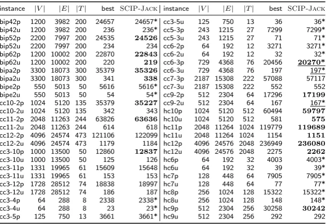
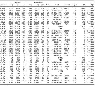
Table 13: Primal bound improvements on the PUC instances
instance |V| |E| |T| best SCIP-Jack instance |V| |E| |T| best SCIP-Jack
bip42p 1200 3982 200 24657 24657* cc3-5u 125 750 13 36 36* bip42u 1200 3982 200 236 236* cc5-3p 243 1215 27 7299 7299* bip52p 2200 7997 200 24535 24526 cc5-3u 243 1215 27 71 71* bip52u 2200 7997 200 234 234 cc6-2p 64 192 12 3271 3271* bip62p 1200 10002 200 22870 22843 cc6-2u 64 192 12 32 32* bip62u 1200 10002 200 220 219 cc6-3p 729 4368 76 20456 20270*
bipa2p 3300 18073 300 35379 35326 cc6-3u 729 4368 76 197 197* bipa2u 3300 18073 300 341 338 cc7-3p 2187 15308 222 57088 57117 bipe2p 550 5013 50 5616 5616* cc7-3u 2187 15308 222 552 552 bipe2u 550 5013 50 54 54* cc9-2p 512 2304 64 17296 17199
cc10-2p 1024 5120 135 35379 35227 cc9-2u 512 2304 64 167 167* cc10-2u 1024 5120 135 342 343 hc10p 1024 5120 512 60494 59797
cc11-2p 2048 11263 244 63826 63636 hc10u 1024 5120 512 581 575
cc11-2u 2048 11263 244 614 618 hc11p 2048 11264 1024 119779 119689
cc12-2p 4096 24574 473 121106 122099 hc11u 2048 11264 1024 1154 1151
cc12-2u 4096 24574 473 1179 1184 hc12p 4096 24576 2048 236949 236080
cc3-10p 1000 13500 50 12860 12837 hc12u 4096 24576 2048 2275 2262
cc3-10u 1000 13500 50 125 126 hc6p 64 192 32 4003 4003*
cc3-11p 1331 19965 61 15609 15648 hc6u 64 192 32 39 39*
cc3-11u 1331 19965 61 153 153 hc7p 128 448 64 7905 7905* cc3-12p 1728 28512 74 18838 18997 hc7u 128 448 64 77 77* cc3-12u 1728 28512 74 186 187 hc8p 256 1024 128 15322 15322*
cc3-4p 64 288 8 2338 2338* hc8u 256 1024 128 148 148*
cc3-4u 64 288 8 23 23* hc9p 512 2304 256 30258 30242
cc3-5p 125 750 13 3661 3661* hc9u 512 2304 256 292 292
have been underlined and marked with an asterisk in Table 13. For a further 16 instances,SCIP-Jackimproved the best known solution. All instances for which the best known primal bound has been improved are marked in bold. Finally, all previously solved instances of the PUC test set have also been solved by SCIP-Jack to proven optimality, which have been marked by an asterisk (without underline).
The instances presented in Table 13 differ widely in their solving behavior. Using the cc6-3u instance as an example, one obtains greater insight into the typical solving procedure when applyingParaSCIP. The cc6-3u instance was solved to optimality for the first time bySCIP-JackandParaSCIP. In order to solve this instance again in a single run without restarting, SCIP-Jack was run on the HLRN-III supercomputer consisting of a Cray XC30. This experiment was performed by using nodes equipped with two 12-core Intel Xeon Haswell CPUs sharing 64 GB of RAM and with a CPU clock of 2.5 GHz. By deploying 3072 MPI processes, the optimal solution with an objective value of 197 was proven in 961 seconds after having processed 123 210 branch-and-bound nodes. While the lower branch-and-bound was already within a distance of one to the optimal objective value after 20 seconds, the primal bound dropped to 198 only after 100 seconds.
5 Conclusions
This paper shows the multilayered impact of embedding a 15-year old Steiner tree branch-and-cut procedure into a state-of-the-art MIP framework and clus-tering new solving methods around it. First, the amount of problem-specific code is drastically reduced. At the same time the number of general solution methods available, e.g., cutting planes, has increased and will be kept up-to-date just by the continuous improvements in the framework. Furthermore, the opportunity to solve instances in a massively parallel distributed memory en-vironment has been added at minimal cost. Attempts were made to solve open instances from the difficult PUC test set by using these massively parallel ex-tensions. As a result,SCIP-Jackwas not only able to solve three previously unsolved instances, but improve the best known solution for another 16.
The use of a general MIP solver allows a significant amount of flexibility in the model to be solved.SCIP-Jackis able to support solving ten variants of the Steiner tree problem with nearly the same code, and the support of further restrictions in the model is straightforward. On top of this versatility, the powerful solving framework for the underlying IP formulation combined with problem-specific methods such as reduction techniques allowsSCIP-Jack to be highly competitive with problem-specific state-of-the-art solvers.
Yet, there certainly is potential for future work to improve the perfor-mance and scope of the solver. First, already implemented routines such as the branching rule could be improved. Second, additional reduction techniques and heuristics for specific Steiner tree problem variants could be implemented. Finally,SCIP-Jackcould be extended to cover further Steiner problem vari-ants described in the literature. By using the plugin structure of SCIP, the inclusion of some of these enhancements is expected in the future.
Ultimately, this paper has described the creation of a highly competitive exact solving framework of outstanding versatility that can veritably be des-ignated as a Steiner class solver. Furthermore, to the best of our knowledge this is the first time that a powerful exact Steiner tree solver has been made available in source code to the scientific community. TheSCIPOptimization Suite [9] already contains a previous version of our solver and the current ver-sion of SCIP-Jack is planned to be part of the next release of SCIP. We hope that the availability of such a device will foster the use of Steiner trees in modeling real-world phenomena.
6 Acknowledgements
The work for this article has been conducted within the Research Campus Modal funded by the German Federal Ministry of Education and Research (fund number 05M14ZAM). It has been further supported by a Google Faculty Research Award.