Neuronal Signal Modulation By Dendritic Geometry

(1)

A Thesis Submitted for the Degree of PhD at the University of Warwick

Permanent WRAP URL:

http://wrap.warwick.ac.uk/129215

Copyright and reuse:

This thesis is made available online and is protected by original copyright.

Please scroll down to view the document itself.

Please refer to the repository record for this item for information to help you to cite it.

Our policy information is available from the repository home page.

(2)

Neuronal Signal Modulation

by Dendritic Geometry

by

Yihe Lu

Thesis

Submitted to the University of Warwick

for the degree of

Doctor of Philosophy

Centre for Complexity Science

(3)

Acknowledgments

First of all, I would like to express my most sincere gratitude to my supervisor, Dr.

Yulia Timofeeva. I started my Ph.D. project with passionate curiosity in nature and

science but mere preparation in the research direction. She has been since then the

most supportive and encouraging person. Discussions with her have always been

enjoyable and pedagogic. My Ph.D. work, as well as my Ph.D. life, has benefited

considerably from her guidance and assistance.

Second, I want to thank Dr. Hugo van den Berg and Prof. Magnus Richardson,

who brought me the initial insight and interest into the field of neuroscience during

my postgraduate study, and all the staff at the Centre for Complexity Science for

their ardent support in my doctoral training. I would also like to thank Dr.

Nicolan-gelo Iannella for inspiring discussions over dendritic resonance and taper, and Dr.

Tom Rother for constructive suggestions on Green’s functions in general cases.

Last but not least, I am grateful to my families and friends. To borrow some

words from Isaac Newton, I have been playing on the seashore, looking for pretty

shells, and knowing nothing about the great ocean of truth. Nonetheless, I do know

I can see stars at night, and they are my families and friends. Amongst them I

dedicate the special thanks to my father, Xiaohe Lu. He has not only offered me

(8)

Declarations

I declare this thesis is my original work, and I gratefully credit all the authors of

the literature that form the foundation of my work. In terms of the copyright issue,

the permissions to reuse the materials in Fig. 1.1, 1.2, 1.3 and 5.1 in this thesis

are granted to me by the publishers. In addition, Fig. 2.4 is reused with minor

modifications at the courtesy of Yulia Timofeeva (one of the authors of the original

material) under a Creative Commons license.

Parts of this thesis have been written up into two papers:

Lu Yihe and Yulia Timofeeva. Response functions for electrically coupled

neuronal network: a method of local point matching and its applications.

Biological Cybernetics, 110(2-3):117–133, 2016.

Lu Yihe and Yulia Timofeeva. Cable theory in neurons with tapered and

branched dendrites. In preparation for submission.

The first paper presents the original development of the method of local point

match-ing, and thus contains the same content as inChapter 2. Nonetheless, the chapter offers more rigorous deductions and more comprehensive explanations. The second

paper derives the generalised sum-over-trips framework for reducible tapers, which

duplicates some sections in Chapter 3. It will be submitted for publication in March, 2019.

This thesis is submitted to the University of Warwick for the degree of Doctor of

(9)

Abstract

Neurons are the basic units in nervous systems. They transmit signals along neurites and at synapses in electrical and chemical forms. Neuronal morphology, mainly dendritic geometry, is famous for anatomical diversity, and names of many neuronal types reflect their morphologies directly. Dendritic geometries, as well as distributions of ion channels on cell membranes, contribute significantly to distinct behaviours of electrical signal filtration and integration in different neuronal types (even in the cases of receiving identical inputsin vitro).

(10)

Abbreviations

IF - Integrate-and-Fire

EPSC - Excitatory Post-Synaptic Current

EPSP - Excitatory Post-Synaptic Potential

LTI - Linear Time-Invariant

RC - Resistor-Capacitor

LRC - Inductor-Resistor-Capacitor

STDP - Spike-Timing-Dependent Plasticity

CR - Coupling Ratio

SDS - Spike-Diffuse-Spike

(11)

Units

ms - millisecond

min - minute

kHz - kilohertz

µm - micrometer

cm - centimeter

nA - nanoampere

mV - millivolt

Ω - ohm

MΩ - megaohm

H - henry

µF - microfarad

(12)

Chapter 1

(13)

1.1 Overview of thesis

A nerve cell, also known as a neuron, is the basic unit in any nervous system. A

human brain, probably the most complex nervous system, consists of approximately 1011 neurons; the number is of the same order as that of the stars in our galaxy, but the interactions among neurons are not dominated by the single force of gravity.

Most neurons shares a typical structure, consisting of a soma (i.e. cell body), an axon and dendrites. Via neurites (i.e. dendrites and axons) and synapses (chemical

or electrical), a typical neuron can connect to and communicate with thousands

of other cells, locally and distantly, forming small neuronal circuits, large neural networks and eventually an entire nervous system. Since the exemplary works of

Ram´on y Cajal [1], scientists started to study the complex branching structures of neuronal dendrites, which is probably the most distinguishable feature of neurons.

As composed by Spencer [2] that, “Everywhere structures in great measure

deter-mine functions; and everywhere functions are incessantly modifying structures”, the interplay between anatomy and physiology in dendrites is evidently vital [3–8]. In

particular, different types of neurons modulate electrical signals differently, because

of their distinct dendritic geometries [5–8].

This thesis tries to understand how dendritic geometry modulates neuronal signal

transmission on a single neuron from a theoretical perspective, mainly by

mathe-matical analysis accompanied with numerical results. Although the functional dif-ferences between neurons are also considerably determined by species of ion channels

on cell membranes [9–16], their types and distributions are completely encoded into

the electrical parameters in the simplified mathematical models of dendritic electro-physiology to be employed in this thesis. In the following sections of thisChapter 1, I will introduce, from a mathematical modelling point of view, neuronal morphology

and electrophysiology respectively in the content of neuroscience in general. These two aspects of dendrites are then brought together and synthesised in the

mathemat-ical formalism “dendritic cable theory” [17]. Chapter 2 will find a mathematical approach to find electrical response functions on neurons of arbitrary dendritic ge-ometry, which is the principal task of this thesis. For simplicity, individual dendritic

branches are modelled by cylindrical segments here. Based on the path integral

for-mulation, the sum-over-trips framework is derived and extended [18–20]. I then develop the method of local point matching, a novel approach to find analytical

(14)

ta-pered dendrites. InChapter 4, I will consider several neuronal models of simplified but representative dendritic geometries. The local point matching method will be employed to calculate the analytical Green’s functions, and then explicit effects of

dendritic geometry on signal modulation will be investigated over the numerical

re-sults. Finally in Chapter 5, I will summarise this thesis, discuss the results and finish by proposing several natural extensions and implications.

1.2 Mathematical modelling of neuronal dendrites

The termdendrite, coined by Wilhelm His in 1889 [21], originates from Greek, which

literally means a tree, or a tree-like form [22]. Scientific investigation on neuronal

dendrites started with Ram´on y Cajal [1], and the classification of neurons by their distinct morphologies is one of the most common and conventional perspectives, e.g.

pyramidal neurons (see Fig. 1.1 for more examples). Such anatomical varieties can

directly lead to functional differences. Computer simulations have shown that, with identical ion channel types and distributions, different morphologies present distinct

signal propagation and firing patterns when responding to the same input currents

(see Fig. 1.2) [6, 7]. However, due to the natural heterogeneous distributions of ion channels on dendrites (and axons) [16], it is difficult to conduct real experiments

on neurons of different morphologies with the ion channel distributions as control

variables. Thus, theoretical approaches as taken by this thesis may help to shed light on the modulation of neuronal signals by dendritic geometries.

This section aims to build mathematical models of dendrites. By “mathematical

modelling”, two interdependent aspects of dendrites are considered: dendritic mor-phology, the geometry of the typical tree structure, and dendritic electrophysiology,

the dynamics of membrane potentials.

1.2.1 Digital reconstructions

To obtain the morphological structure of a real neuron,neuron tracingis employed

by neuroscientists. It has become one of the most fundamental tasks in neuroscience,

particularly in computational neuroscience, as digital reconstructions obtained by neuron tracing are useful in computer simulations on single neurons or neural

net-works with realisitic neuronal morphologies [24]. There are online databases

nowa-days, e.g. Neuromorpho.org [25], which permit access to numerous neuron recon-tructions.

Conventionally, neurons are stained and imaged in fixed brain tissue by the

(15)

[image:15.595.125.516.108.357.2]

Figure 1.1: Distinct morphologies of different neurons. (A): Alpha motor neuron in spinal cord of cat. (B): Spiking interneuron in mesothoracic ganglion of locust. (C): Layer 5 neocortical pyramidal neuron in rat. (D): Retinal ganglion neuron in postnatal cat. (E): Amacrine neuron in retina of larval tiger salamander. (F): Cerebellar Purkinje neuron in human. (G): Relay neuron in ventrobasal thalamus of rat. (H): Granule neuron in olfactory bulb of mouse. (I): Spiny projection neuron in rat striatum. (J): Neuron in the Nucleus of Burdach in human fetus. (K): Purkinje neuron in mormyrid fish. (L): Golgi epithelial (glial) neuron in cerebellum of normal-reeler mutant mouse chimera. (M): Axonal arborization of isthmotectal neurons in turtle. Copied from [23].

and is still in use by modern neuroscientists, whereas recent developments permit functional imaging [26, 27]. The work of Glaser and Van der Loos [28] is one of

the first attempts on automation in neuron tracing. They employed computers to

interact with the microscope and to store point coordinates, which were manually indicated by a human operator. In spite of many efforts to reduce the amount

of human labour [29, 30], neuron tracing had remained as a difficult problem (see

Fig. 1.3) [31, 32] until tremendous progress in the fields of computer science and computer vision occured in the recent years [33].

Instead of directly recording neuronal morphologies by some automatic process,

nowadays it is preferred to acquire the entire image data first. These image data are initially refined by several image preprocessing techniques so that segmentation

(16)

[image:16.595.124.515.175.516.2]

(17)

[image:17.595.195.450.105.347.2]

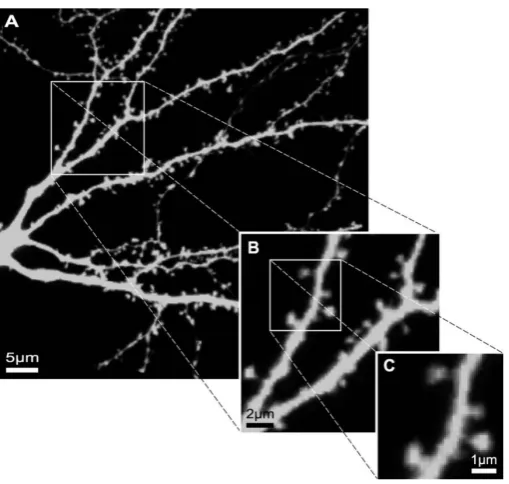
Figure 1.3: The multiscale nature of a dendritic tree. (A): The level of a individual neuron. (B): The level of dendritic branches and bifurcations. (C): The level of individual spines. While this is a fairly high-quality data set, several branches are still poorly stained in (A) and spines in (C) are usually poorly imaged due to the limited resolution and can be further blurred by noises, in particular in live-cell imaging experiments, thereby causing visual ambiguities and enhancing the complexity of the problem. Copied from [33].

soma, especially in the case where multiple neurons are present, neurites are the next to be tracked, and finally spines are detected [33]. The processing order is not only

heuristic but also insightful, because a successive step can employ or even rely on the

results of its preceding steps. After measuring parameters for all segments identified, automatic tracing is complete. It is however more rigorous to conduct proof-editing

at this stage, because structural errors in reconstructions, if not corrected, could

potentially take researchers more time to find out than conducting manual tracing [34].

One may run realistic computer simulations on such neuron reconstructions, e.g.

the reconstruction in Fig. 1.4 employed by [19]. One may also conduct experiments by simulations that are nearly impossible in reality but insightful in theory. For

example, the reconstructions shown in Fig. 1.2 are modelled with identical ion

chan-nels for different morphologies [6, 7]. The digital reconstruction of a neuron usually preserves the most comprehensive information of its three-dimensional morphology.

(18)

[image:18.595.124.517.108.247.2]

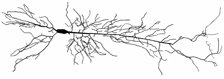
Figure 1.4: A reconstructed neuron from a rat CA1 hippocampal pyramidal cell. The reconstruction consists of 396 branches and a soma and is compartmentalised into 3961 cylindrical segments. Adapted from [19].

is extremely difficult, and numrical simulations are computationally expensive. As a

result, there are very few but grand projects, e.g. the Human Brain Project [35], that

does simulate a “large” network with such morphologically detailed neurons, in the hope of shedding light on the biological foundation of consciousness and intelligence.

For example, Markram et al. [36] simulated a microcircuitry of the somatosensory

cortex in a juvenile rat, which contains approximately 31,000 neurons.

1.2.2 Simplified geometries

To clearly exhibit branching structures of dendrites, adendrogramis conventionally

employed. Dendrograms are firstly introduced by Sholl [37] and thus are also known as Sholl diagrams (see Fig. 1.5 for an example). In order to draw theoretical insights

and to save computational expenses, morpohologies of neuron reconstructions can

be simplified and often considered as multi-compartment models (see schematic diagrams in Fig. 1.6). Since such a multi-compartment model virtually spans in

a two-dimensional plane, the morphology of a neuron can be formally modelled as

a weighted graph Γ = (N,B), in particular a weighted tree. Its vertices represent soma and branching nodes, and the edges represent dendritic branches. Moreover, Γ

is a metric graph, as the weights of its edges are assigned to be the physical lengths

of the corresponding branches. Based on this mathematical definition, methods of graph theory can be employed to study the dendritic geometry, e.g. algorithms for

finding minimum spanning trees [38, 39].

It is practical and reasonable to study such simplified models for two main rea-sons. First, it is in principle impossible to acquire perfect details of dendritic

(19)

[image:19.595.125.516.109.443.2]

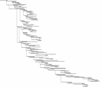
Figure 1.5: Dendrogram of the pyramidal cell shown in Fig. 1.4. Each horizontal segment represents a dendritic segment with its physical length and each vertical segment corresponds to a branching point.

a dendritic tree is constantly changing its structure due to the motility of

den-dritic spines [40]. Second, it is relatively straightforward to investigate neuronal electrophysiology (to be introduced in§1.2.3) on simplified morphologies by either

mathematical analysis or computer simulations.

To further simplify dendritic geometry, one may consider a point neuron without any branching structure. It can be treated as the most extremely reduced model with

only one compartment (see Fig. 1.6), or an isopotential neuron whose dendrites and axons function with instant signal propagation, communicating with other point

neurons via metaphysical synapses. Although this thesis does not consider point

neurons because there are virtually no dendrites, they are useful in studying mod-els of neuronal membrane potential dynamics (see §1.2.3). In addition, since the

(20)

[image:20.595.129.518.111.373.2]

Figure 1.6: Schematic diagram of morphological model reduction at different leveles of the pyramidal cell shown in Fig. 1.4 (up to rotation), from 397 compartments (leftmost), down to 26, 4, and only 1 compartment (rightmost). Although the soma (represented by a disc) in each model here is an isopotential compartment, it is not necessarily the case. For example, the soma in the reconstruction in Fig. 1.4 (which is essentially a multi-compartment model as well) consists of 3 segments.

artificial neural networks consisting of point neurons have proven themselves efficient and powerful in many applications. For example, the automation and digitalisation

of neuron tracing mentioned in§1.2.1 have largely benefited from the development

of techniques in pattern recognition in the field of machine learning, which heavily employs artificial neural networks.

1.2.3 Membrane potentials

Cell membranes separate intra-cellular plasma from extra-cellular environment in order to maintain cellular homeostasis. Neuronal membranes, in particular,

mod-ulate the flows of charged ions selectively by its pore-forming membrane proteins.

There are thus differences in ionic densities at the two sides of neuronal membranes, which create a difference between intra- and extra-cellular electric potentials, i.e.

membrane potentials. To study the dynamics of membrane potentials, a quantative

(21)

[image:21.595.199.440.104.353.2]

Figure 1.7: A circuit diagram of a general conductance-based model. The membrane potentialV is the voltage difference between the intra- and extra-cellular potentials, which is measured at the lipid bilayer, represented by a capacitor. The membrane leakage is analogous to the series circuit of a resistor gl and a battery El, and a voltage-gated ion channel of ionic species k is the series circuit of a non-linear voltage-dependent conductor gk(V) and a battery Egk. If there are multiple ionic species, they are all parallel circuits to one another.

Notably, here a point neuron (introduced in§1.2.2) is assumed, and notations and terms from control theory.

Capacitors: lipid bilayer

The cell membrane of a neuron is a lipid bilayer, which prevents ions at the both

sides moving freely across it. It thus behaves as a capacitor, that is, it can be

charged up by an injection of a current Im (generally varying with respect to time t) into the plasma, or mathematically,

Im(t) =CmAm dV

dt , (1.1)

(22)

Resistors: leakage channels

The lipid bilayer of the cell membrane is not perfectly dielectric, and at the same

time there areleakageion channels that allow selective ionic species to travel across

the membrane. In reality most of leakage channels behave as rectifiers, that is, they conduct better in one fixed direction than the other. Nonetheless, leakage channels

are simply assumed to be resistors (i.e. linear conductors). As they follow Ohm’s

law, the leakage current can be written as

Il(t) =

X

k

g_lkAm(V −Elk), (1.2)

whereg_lk is the leakage conductance per unit area and E_lk is the reversal potential of ionic speciesk. Since both g_lk and E_lk are constants predetermined by the ionic speciesk, the leakage current (1.2) can be therefore recast into a simpler form,

Il(t) =glAm(V −El), (1.3) where

gl=

X

k gk_l is the total leakage conductance per unit area, and

El =

P

kglkElk gl is the passive resting membrane potential.

If the membrane potential of a point neuron is determined only by the currents

(1.1) and (1.3), Kirchhoff’s current law gives

Im(t) +Il(t) =I0(t), (1.4) where I0(t) is the input current. The neuron in this case is purely passive. It is equivalent to a resistor-capacitor (RC) circuit, whose output voltage, i.e. solution to Eq. (1.4), is proportional to an exponential-filtered input current.

Inductors: h-channels

(23)

hyperpolarisations. Theh-channels can be modelled as inductors, that is, Lh

Am dIh

dt =− rh Am

Ih+ (V −El), (1.5) whereLh is the inductance andrh the resistance per unit area.

The neuron whose membrane potential dynamics is determined by the currents

(1.1), (1.3) and (1.5) is analogous to an resistor-inductor-capacitor (RLC) circuit,

which is also known to be aresonant circuit. It is explicitly described by

Im(t) +Il(t) +Ih(t) =I0(t), (1.6) whereI0(t) is the input current, and Kirchhoff’s current law is applied.

Non-linear conductors: voltage-gated channels

To explain the initiation and the propagation of action potentials in the squid giant axon, the Hodgkin-Huxley model [42] considers a conductance-based model

consist-ing of the currents (1.1), (1.3), and the followconsist-ing two non-linear ion channels,

INa= ¯gNam3h(V −ENa), (1.7a) IK= ¯gKn4(V −EK), (1.7b) where ¯gk = gkmaxAm is the maximal conductance for ionic species k ∈ {K,Na} (potassium and sodium),Amis the surface area of the membrane, andn, m, h∈[0,1] are gating variables for the activation of potassium channels, the fast activation and

the slow inactivation of sodium channels, respectively.

In general, such voltage-gated ion channels can be modelled as non-linear con-ductors, which permit the following current through these channels,

Ig(t) =

X

k

g_maxk wk(V)Am(V −Egk), (1.8)

where, for each ionic speciesk,g_maxk is the maximal active conductance per unit area, E_gkis the reversal membrane potential, andwk(V)∈[0,1] describes the fractions of channels that are open. For any ion speciesk, in general,

wk(V) =Y i

nηi

i ,

(24)

or inactivation at different time scales which changes in V, and ηi is the number of the independent (in)activation gates of the channel. Assumeαni(V) the opening

rate (the transition rate that a channel changes its gating state from close to open)

andβni(V) the closing rate. The gating variable follows

dni

dt =αni(V)(1−ni)−βni(V)ni, (1.9)

which can be recast as

τni(V)

dni dt =w

k

∞(V)−ni, (1.10) where

τni(V) =

1

αni(V) +βni(V)

, (1.11)

ni,∞(V) =

αni(V)

αni(V) +βni(V)

. (1.12)

Thermodynamics suggests the shape of ni,∞(V) to be a sigmoid function [43],

whereas αni(V), βni(V) and ηi can only be obtained by fitting models with

experi-mental data. A general conductance-based model can then be obtained by applying Kirchhoff’s current law with the currents (1.1), (1.3) and (1.8), plus an input current

I0(t), that is,

Im(t) +Il(t) +Ig(t) =I0(t). (1.13) Sincewk(V) is dependent onV, the current Ig(t) is non-linear, and thus the model is not analytically solvable, whereas the non-linear current can be approximated by a linearised current (in a similar form to Ih) if small enough [19, 44].

Batteries: reversal potentials

The reversal potentials E_lk, E_gk in Eqs. (1.2) and (1.8) are analogous to batteries in the electrical circuit. A reversal potential Ek of an ionic species k is defined to be the membrane potential at which the net flow across membrane is zero. It can be derived directly from this definition and is explicitly given by the famous Nernst

equation,

Ek = kBT zkq

log

N_ke N_ki

,

(25)

constant from the beginning of all neuronal models in this thesis.

1.2.4 Cable theory

In 1952, Hodgkin and Huxley [42] successfully explained the initiation and the prop-agation of action potentials in the squid giant axon by a cable equation with

non-linear voltage gated channels. The model was a milestone in the development of

neuronal cable theory, it won Hodgkin and Huxley a Nobel Prize in 1963, and it has been since known as the Hodgkin-Huxley model. As a matter of fact, about a

century before that, Von Helmholtz [46] experimentally measured the signal veloc-ity in nerve fibers of a frog, and only a few years later Thomson [47] developed the

prototypic cable theory to study transmission of telegraphic signals in long cables,

which established the theoretical foundation of cable theory but its relevance to neuronal cables was not noticed upon that time. With the development of sharp

micropipette electrodes, dynamics of dendritic membrane potentials also started to

be revealed by intra-cellular recordings, and their observations can be elaborated by

dendritic cable theory. The theory was thoroughly studied by Wilfrid Rall, whose

significant contribution to the topic is well summarised in the book of Segev et al.

[48]. Classical cable theory essentially extends the models for a point neuron (dis-cussed in §1.2.3) to a neuronal cable [49, 50], and dendritic cable theory aims to

apply cable theory on a complex dendritic morphology.

It is ideal to build models of dendritic membrane potential dynamics in the three-dimensional space, because “any other approach risks excluding important features

of the three-dimensional structure or incorporating three-dimensional features

incor-rectly” [51]. Nonetheless, the standard cable equation is one-dimensional in space, since all radial currents are assumed to be transmembrane, an assumption can be

justified by the fact that the diameter of a typical neurite is considerably small

com-paring to its length [52]. It is also shown in [51] that the one-dimensional standard cable equation is the limit of their three-dimensional model given common

assump-tions. Below I first derive the general cable equation of a single dendritic branch

with continuously varying radius r(x), into which an input current Iin(x;t) is ap-plied. It is then straightforward to obtain the classical standard cable equation and

(26)

General cable equation

To begin with, I focus on a little section of the dendritic branch fromx tox+ ∆. Kirchhoff’s current law (the conservation of electrical currents at a point) gives

Im(x) +Il(x) +Ig(x) +I(x+ ∆) +Iin(x+ ∆) =I(x) +Iin(x), (1.14) where I(x) is the axial current flowing into the section and I(x+ ∆) is the axial current flowing out. The other currents can be found in Eqs. (1.1), (1.3) and (1.8). Substituting them into Eq. (1.14) leads to

Cm ∂V

∂t +gl(V−El)+

X

k

g_maxk wk(V−E_gk) = I(x)−I(x+ ∆) +Iin(x)−Iin(x+ ∆) Am(x, x+ ∆)

, (1.15) where the surface area of the section is

Am(x, x+ ∆) = 2π

Z x+∆

x

ρ(s)ds, (1.16) and

ρ(s) =r(s)p1 + (r0(s))2_, _(1.17) as the cross-sectional area is assumed to be perfectly round. Only the right hand

side of Eq. (1.15) depends on ∆ and thus by taking the limit ∆↓0,

lim ∆↓0

−[I(x+ ∆)−I(x) +Iin(x+ ∆)−Iin(x)]/∆

Am(x, x+ ∆)/∆

=−∂I/∂x+∂Iin/∂x

2πρ(x) . (1.18) If the input current of a total strength ofIinj is injected only into the section from y toy+ ∆, given the same limit ∆↓0,

∂Iin ∂x

y+

=−Iinjδ(x−y), (1.19)

whereδ(x−y) is the Dirac delta function. Without loss of generality, from now on all input currents are assumed to be point processes. It is worth noting that the

results for a region of input can be recovered by integrating over the input region.

At the same time, the axial current I(x) flowing through the section can be calculated by Ohm’s law, that is,

V(x+ ∆)−V(x) =−I(x)R, R= Ra∆ 2

Rx+∆

x Ac(s)ds

(27)

whereRa is the axial resistivity and Ac(x) = πr2(x) is the cross-sectional area. It follows from the above equations that

I(x) =−

Rx+∆

x Ac(s)ds Ra∆

V(x+ ∆)−V(x)

∆ ,

and again with the limit ∆↓0,

I(x) =−1

ra ∂V

∂x, (1.21)

where

ra(x) = Ra

πr2₍_x₎, (1.22)

is the axial resistance. Thus,

∂I ∂x =−

π Ra

∂ ∂x

r2(x)∂V ∂x

. (1.23)

The general cable equation of a radius-varying dendritic cable with non-linear

chan-nels are obtained by substituing Eqs. (1.19) and (1.23) into Eq. (1.18), that is,

Cm ∂V

∂t =−gl(V−El)−

X

k

g_maxk wk(V−E_gk) + 1 2Raρ(x)

∂ ∂x

r2(x)∂V ∂x

+I0, (1.24)

where

I0 =

Iinjδ(x−y)

2πρ(x) (1.25)

could be considered as the driving force in Eq. (1.24), and is notably determined

only by the input locationy (not x), because δ(x−y) = 0 if and only if x=y.

Simplified cable equations

As most of voltage-gated channels are non-linear, Eq. (1.24) is generally impossi-ble to solve analytically. Nonetheless, in the sub-threshold regime, they could be

linearised (see§1.2.3). For simplicity, here I consider onlyh-channels which permit Ih currents. Substituting the non-linear currents (1.24) by the Ih current (1.5), the

resonant (quasi-active) tapered cable equationis obtained,

Cm ∂V

∂t =−glV −Ih+ 1 2Raρ(x)

∂ ∂x

r2(x)∂V ∂x

+I0, (1.26a) Lh

∂Ih

(28)

where notably the membrane potential is from now on measured fromEl.

A further simplification is to remove the Ih current from the model. It can be experimentally realised by blocking theh-channels, and is mathematically equivalent to take the limitrh→+∞. The passive tapered cable equationis thus obtained,

Cm ∂V

∂t =−glV + 1 2Raρ(x)

∂ ∂x

r2(x)∂V ∂x

+I0. (1.27) An alternative simplification of the system (1.26) is to assume constant dendritic radiusr(x) =rcwhile keeping theIh current in the model, which gives theresonant

cylindrical cable equation,

Cm ∂V

∂t =−glV −Ih+ rc 2Ra

∂2V

∂x2 +I0, (1.28a) Lh

∂Ih

∂t =−rhIh+V. (1.28b)

Reducing the model with both simplifications results in thepassive cylindrical cable

equation, i.e. the classical standard cable equation,

Cm ∂V

∂t =−glV + rc 2Ra

∂2V

∂x2 +I0, (1.29)

or, in a more well known form,

τm ∂V

∂t =−V +λ 2∂2V

∂x2 + I0 gl

, (1.30)

where

λ2= rc 2glRa

, (1.31)

and τm = Cm/gl is defined by Eq. (5.4). It is worth noting that the tapered cable equations (1.26) and (1.27) work for general radius-varying dendrites as clearly

shown in the derivation, not only for “tapered cables”. The term “taper” is chosen

because the tapered dendrites are to be investigated in more details inChapter 3. This thesis mainly studies these simplified cable equations (1.26), (1.27) and (1.28)

due to their mathematical tractability.

Input currents

An input current can be produced due to synaptic activities, or directly from exper-imental injection. An input current in either case is considered as a point process

(29)

de-0 100 200 300 -0.3

-0.2 -0.1 0 0.1 0.2 0.3

0 100 200 300

0 0.1 0.2 0.3 B

A

m

p

li

tu

d

e

(

n

A

)

C

0 100 200 300

0 0.5

1 _A

Time (ms)

Figure 1.8: Current profiles of three types of inputs with A0 = 0.2 nA. (A): An EPSC modelled by an alpha function (1.32) withB0 = 0.1. (B): A rectangle input (1.33). (C): A chirp current (1.34) withωchirp = 0.003 kHz.

termined byIinj(t). If I0 = 0, the cable equations (1.26) - (1.29) are homogeneous differential equations. Since they are all linear, the solutions to the corresponding heterogenous equations with different I0 6= 0 are additive. Therefore, it is straight-forward to generalise the input from a point process to a field.

The time profiles of Iinj(t) can vary from cell to cell due to different synaptic activities, or from case to case under different experimental protocols. For simplicity,

an excitatory post-synaptic current (EPSC) can be modelled by the alpha function

(see Fig. 1.8A) [53–56],

IEPSC(t) =A0te−B0t, (1.32) for t = 0 the time the post-synaptic neuron starts to depolarise due to synaptic activities. The function reaches the maximal value of A0(B0e)−1 at time t=B0−1. However, any post-synaptic current is actually dependent on the temporal

mem-brane potential at its location; Eq. (1.32) is notably an extremely simplified model of an EPSC in the case of no shunting currents that would have varied the membrane

conductance are presented. This model can be useful for experiments investigating

single neurons in vitro, whereas it is probably unrealistic for neurons in vivo, since they could constantly receive signals from thousands of synapses.

In addition, rectangle inputs and a chirp currents (see Fig. 1.8B,C) are also widely employed in experiments to investigate the asymptotic and oscillating behaviours of

electrical systems respectively. The rectangle input can be described by

(30)

0 1 2 3 4 5 6 7 8 9 10 260

280 300 320 340

Frequency (kHz)

[image:30.595.224.419.108.264.2]

Amplitude (nA)

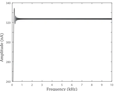
Figure 1.9: Amplitude of the chirp current in Fig. 1.8B in the Fourier frequency domain.

time of the stimulus, and τrect is its duration. If τrect → +∞, the input becomes a step current. A step current drives a neuron to some new steady-state voltage.

It can be employed to find input and tranfer impedances (see §1.3.2) and is thus

usually a primary indicator of signal attenuation on dendrites. The chirp current can be defined as

Ichirp(t) =A0sin ωchirpt2

, (1.34)

whose instantaneous frequency can be found as

f(t) = 1 2π

d

dt ωchirpt 2

= ωchirp π t,

where ωchirp/π is the chirpyness, i.e. the rate of frequency. As the frequency is varying linearly in time, Eq. (1.34) particularly defines a linear chirp. Since the amplitude of the response in the Fourier domain is almost constant for a wide range

of frequencies (see Fig. 1.9), which implies that the power spectrum of the chirp

input is similar to that of a Dirac delta impulse, the envelope of the corresponding oscillating response in time domain roughly traces the Green’s function (which is

by definition the response of a Dirac delta input). Therefore, such chirp inputs

are useful in experiments to characterise resonant systems. It is worth noting that, however, the phases of a chirp input and a Dirac delta impulse are different, and

thus the chirp responses cannot provide an accurate experimental measurement of

(31)

Boundary conditions

Membrane potential dynamics on all individual branches of a dendritic tree are

mod-elled by the system (1.26) in this thesis, whereas different branches in general have

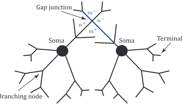
different morphological or electrophysiological parameters. Moreover, four types of boundary conditions (see Fig. 1.10) are considered. They are enforced at the nodes

where dendritic branches are connected or terminated. All boundary conditions are

determined by two physical contraints, Kirchhoff’s current law and the continuity of membrane potentials. The study of dendritic cable theory in this thesis is

basi-cally the mathematical analysis of the system (1.26) given all boundary conditions.

Notably in this section the spatial coordinate is changed case by case so that the boundary under investigation is at the locationx= 0, whereas it is common to fix the coordinate globally when studying a particular neuronal model.

A terminal is the end of a dendritic branch. It is assumed to be either open or

closed. An open terminal means that there is no barrier for ions to move freely

into or out from the neuron, which corresponds to the situation where the dendritic branch is cut off at x= 0. Mathematically,

V(0;t) = 0. (1.35)

In this thesis I assume the terminal of a natural dendritic branch is closed, that is, there are no axial currents atx= 0, which gives

∂V

∂x(0;t) = 0. (1.36)

A branching node is a point at which several dendritic branches are attached

together. Assume there are N branches attached to the point x = 0. The two conditions for axial currents and membrane potentials respectively give

N

X

i=1 1 ra,i(0)

∂Vi

∂x(0;t) = 0, (1.37) Vi(0;t) =Vj(0;t), (1.38) for i, j ∈ {1,2,3, . . . , N} indexing the different branches, where ra,i is the axial resistance for branchi, whose definition can be found in (1.22).

A soma is treated as an isopotential sphere that is mathematically equivalent to the model of a point neuron as in §1.2.3. Similarly only the resonant model is

(32)

Soma Soma Gap junction

Branching node

[image:32.595.172.476.109.284.2]

Terminal

Figure 1.10: A schematic of a network of two neurons connected by a gap junction.

the somatic parameters CS = CsomaAsoma, gS = gsomaAsoma, LS = Lsoma/Asoma, rS =rsoma/Asoma, the explicit conditions for the somatic node can be written as

CS ∂VS

∂t =−gSVS+ N

X

i=1 1 ra,i(0)

∂Vi

∂x(0;t)−IS(t), (1.39a) LS

∂IS

∂t =−rSIS(t) +VS(t), (1.39b) VS(t) =Vi(0;t), (1.39c) whereVS is the somatic membrane potential,ISis the somatic resonant current, and Vi is the membrane potential of the dendritic branch i. Eqs. (1.39a) and (1.39b) are imposed by the Kirchhoff’s current law and Eq. (1.39c) by the continuity of

membrane potentials.

In addition, electrical synapses are considered, which are also known asgap junc-tions. A gap junction is a mechanical coupling between adjacent neurons that

permits direct ion flows between them without a orientation preference, which can be simply modelled by resistors whose conductance is gGJ = R−_GJ1 [20]. This as-sumption is able to elaborate the observations that a signal passing through a gap

junction always attenuates but is almost instant. Explicitly, it follows Ohm’s law,

1 ra,m

∂V_m−

∂x (0;t) + ∂V_m+

∂x (0;t)

=gGJ(Vm−(0;t)−V_n−(0;t)), (1.40a)

1 ra,n

∂Vn−

∂x (0;t) + ∂Vn+

∂x (0;t)

(33)

wherem−andm+ (n−andn+) are the two segments of dendritic branchm(branch n) before and after the gap junction. At the same time, the membrane potentials are continuous on the same branches, that is,

V_m−(0;t) =V_m+(0;t), (1.41a)

V_n−(0;t) =V_n+(0;t). (1.41b)

We can thus consider not only a single neuron, but also multiple neurons coupled by gap junctions, while keeping the entire model relatively simple.

1.3 Solutions by Green’s function formalism

In order to obtain the solution to the cable equations, a classical approach is to solve them without the input currentsI0 first. For example, Eq. (1.29) withoutI0 is simply a one-dimensional heat equation (with an additional term of heat loss), which is homogeneous. It can be solved analytically by separation of variables.

I0 can be then added back into the system, playing a role of initial and bound-ary conditions. Alternatively, the Green’s function formalism is employed in this thesis to solve the resonant tapered cable equation (1.26) and its simplifications,

because they are all diffusion equations that can reduce to Helmholtz equations,

whose Green’s function is known. A Green’s function is an impulse response to an inhomogeneous linear differential equation. It is conventionally a tool for solving

inhomogeneous linear differential equations, first developed by and thus later named

after the British mathematician, George Green [57]. While the term fundamental solutionis preferred instead in modern mathematics, especially in distribution

the-ory [58], Green’s functions are still commonly employed in many-body problems in

physics, and are calledpropagators when it comes to quantum mechanics [59, 60]. In control theory (or linear time-invariant theory), transfer functions, a term

ap-pearing regularly in frequency domain analysis, are no more than Green’s functions

in the frequency domain [61]. In this thesis the termGreen’s functionis consistently employed, whereas occasionally I refer to the other terms when linking to works of

others.

In general, a Green’s function is defined as,

(34)

linear differential equations of the form,

Lu(α) =f(α),

whereα, β∈_Rn_{, because the solution can be directly written as} u(α) =

Z

G(α, β)f(β)dβ+f0, (1.43) wheref0 is a constant, often determined by initial conditions, or simply,

u=G∗f+f0, (1.44)

where ∗ represents the convolution of the two functions. In this thesis, f(β) = I0(x;t) represents input currents into a dendritic tree at some location and time, while u(α) = Vm(x;t) represents output membrane potentials measured at some other location and time. This thesis is focused on finding Green’s functions on

dendritic trees, because they establish direct and complete relations between input currents and output membrane potentials, and encode all together the information

of dendritic geometrical and electrophysiological properties. Formally, I consider

the geometry modelled by a metric graph Γ = (V, E) for V the set of vertices and E the set of edges in the graph. Since each edge e ∈ E is equipped with a differential operatorDe acting on the function of membrane potential dynamics, Γ is a quantum graph (see [62, 63] for a review). Therefore, in mathematical terms, this thesis attempts to find the following mapping,

M: (Γ, α, β)→GΓ(α, β), (1.45) which determines the Green’s function GΓ for any Γ that satisfies the modelling criteria in this thesis, given arbitrary output-input pairs (α, β). The differential operatorDein this thesis is mainly the Helmholtz operator. Their Green’s functions can be constructed by the path integral formulation, that is, the Green’s function GΓ(α, β) is found by summing over all the random walk paths between α and β on the quantum graph Γ. Notably I consider only the deterministic limit in this

thesis, whereas realistic neuronal membrane potential dynamics is stochastic. By the law of large numbers, it should be justified that such deterministic limits well

(35)

1.3.1 Properties of Green’s functions

Below several important properties of Green’s functions are discussed. They

gener-ally work for any linear systems.

A chain of convolutions

Assume L=L1L2 and G1, G2 are the Green’s functions of L1, L2 respectively. By applying Eq. (1.44) twice with respect toL1, L2 in order,

u=G2∗G1∗f, (1.46)

and, ifGis the Green’s function of L,

G=G2∗G1, (1.47)

or explicitly,

G(α, β) =

Z

G2(α, ζ)G1(ζ, β)dζ. (1.48) By mathematical induction, the corollary of a chain of convolution follows,

G=GN ∗GN−1∗ · · · ∗G2∗G1, (1.49)

if L = L1L2L3. . . LN, where Gk is the Green’s function of the linear operator Lk fork∈ {1,2,3, . . . , N}, and G is the Green’s function ofL.

Linear time-invarient system

The resonant cable equation (1.26) is by definition a linear system. It is also easy to

see that the system is time-invariant because all the coefficients in the differential equations are constant in t. It is thus a linear time-invariant (LTI) system, whose Green’s function with respect tot can be rewritten in a convenient way, that is,

G(t, t0) =G(t−t0). (1.50) Moreover, an LTI system can be completely characterised by the Green’s function,

because the output is simply

u(t) =

Z ∞

−∞

(36)

Due to Eq. (1.49), Eq. (1.50) can be extended to a series of time pointst0, t1, t2, . . . , tN =t,

G(t, t0) =G(t−t0) =G(t−tN−1)G(tN−1−tN−2). . . G(t2−t1)G(t1−t0). (1.52)

Additivity of multiple inputs

The additivity of multiple inputs is essentially determined by the linear operator,

which leads to

V(x,y;ω) =G(x,y;ω)I0T(y;ω), (1.53)

wherey= (y1, y2, y3, . . . , yN) is an array ofN input locations, andG,I0 are arrays

of size N whose individual elements are successively defined by the corresponding elements ofy. Moreover, Eq. (1.53) can be easily rewritten into an integration form iny, by assuming the points of y locate closely in a certain region and taking the limit so that these points are continously distributed, that is,

V(x, y;ω) =

Z

G(x, y;ω)I0(y;ω)dy, (1.54) whereI0(y;ω) is a region of input that has a continuous density in amplitude. This enables calculation of general inputs directly from the point processes assumed by Eq. (1.19).

Notably the property (1.53) is purely a mathematical result, which is

approxi-mately valid only if the individual inputs are small or distant enough. For example, when an experimentalist injects a single current into a dendritic branch. However,

it has been long since the existence of non-linear interactions of synaptic inputs on

dendrites were discovered [64], and a typical neuronin vivocould constantly receive thousands of inputs due to synaptic activities. A single input is assumed throughout

this thesis; I will leave the discussion of such non-linear behaviours in§5.1.5.

Reciprocity between input and output

Since the resonant cable equation (1.57) (in the frequency domain) is a second order linear ordinary differential equation, it can be rewritten in the Sturm-Liouville form.

Since the Sturm-Liouville operator is self-adjoint, the Green’s function must be

symmetric [65], that is,

(37)

Nonetheless, I will give an alternative proof of the reciprocity on dendrites in§2.3.3.

1.3.2 Laplace and Fourier transforms

The Laplace transformLof a function f(t) is defined as F(ω) =L{f(t)}=

Z ∞

0

f(t)e−ωtdt, (1.56) whereω is the complex frequency.

Applying the Laplace transform on Eq. (1.26) results in

E(ω)V(x;ω) = 1

2Raρ(x) ∂ ∂x

r2(x)∂V(x;ω) ∂x

+I0(ω) +U0(ω), (1.57) where

E(ω) =Cmω+gl+ 1 rh+Lhω

, (1.58)

U0(ω) =CmV(t= 0) +

LhIh(t= 0) rh+Lhω

. (1.59)

As it is an LTI system, it is safe to assume zero initial conditions, that is, V(t = 0) =Ih(t= 0) = 0, which gives U0 = 0. Since a Green’s function in the frequency domain is one-to-one correspondence to a Green’s function in the time domain, it

completely characterises the system. In addition, convolution in the time domain is

equivalent to multiplication in the frequency domain, that is, Eq. (1.51) becomes

u(ω) =G(ω)f(ω), (1.60) which is easier to analyse and compute.

To recover the function in time domain, the inverse Laplace transfrom L−1 _is employed,

f(t) = 1 2πi

Z c+i∞

c−i∞

F(ω)etωdω, (1.61) for c an arbitrary real number that guarantees the coutour integration to be con-vergent with respect toF(ω).

At the same time, the Fourier transform is defined as

ˆ f(¯ω) =

Z ∞

−∞

(38)

in general treated as complex, in which cases the two transforms (1.56) and (1.62)

are indifferent as long asf(t) = 0 fort <0, which is assumed throughout this thesis. If ¯ω is real valued, the Fourier frequency is then merely the complex component of the Laplace frequency, which characterises the periodic behaviours of the system,

while the real component of the Laplace transform is responsible for the transient behaviours. Moreover, the inverse Fourier transform,

f(t) = 1 2π

Z ∞

−∞

ˆ

f(¯ω)e−itω¯dω,¯ (1.63) is equivalent to the inverse Laplace transform (1.61), if c can be chosen as zero, that is, if all singularities are in the left half-plane. It is worth noting that this

condition roughly implies that there exists someF(ω), such thatccannot be set as zero, in which cases the inverse Fourier transform will not converge. However, this

thesis does not give any mathematical proof on whether or not the two transforms

are interchangeable for any particular Green’s function, because it will be easier to check the convergence after obtaining explicit expressions.

Although the terminology for the Laplace transform will be employed for

consis-tency, it is more convenient particularly in numerical integrations to use the Fourier transform because algorithms of the fast Fourier transform (and its inverse) is

effi-cient and accurate.

Final values of responses

By injecting a step current into a neuron, it is expected that the entire system finally reaches some steady state. AssumeIinj(t) =Istep(t) is the step input of strengthA0 occuring at timet0. It is the special case of a rectangle input (1.33), whose Laplace transform can be found as,

Istep(ω) = A0 ω e

−t0ω_. _(1.64)

In order to obtain the final value, thefinal value theorem for the Laplace transform

can be applied, which states that,

limt→∞f(t) = limω→0ωF(ω), if all poles of ωF(ω) are in the left half-plane. By the theorem,

(39)

which simply gives

lim

t→∞V(x, y;t) = limω→0ω

G(x, y;ω)A0 ω e

−t0ω

=A0G(x, y;ω= 0). (1.66) For a passive systemG(x, x;ω= 0) is by definition the input resistance atx, because A0 in the strength of the injected current and limt→∞V(x, x;t) is the steady state

voltage. However, this measure cannot fully characterise a resonant neuron, as

overshoots and undershoots are to be observed before the system reaches to its steady state.

In order to account for the oscillating behaviours of a neuron, a sinusoidal signal

of the following form,

Isin(t) =A0sin(ω0t), (1.67) can be applied to the system. The system will reach a sinusoidal final state,

VSS(x, y;t) =B0sin(ω0t+φK), (1.68) where the amplitude,

B0 =A0|K(x, y;ω)|, (1.69) and the phase shift,

φK = arg(K(x, y;ω)), (1.70) can be found withK(x, y;ω) =G(x, y; ¯ω) where ¯ω=iω for real ω [61].

Therefore, the Green’s function can be obtained experimentally by measuring the sinusoidal final state responses to sinusoidal inputs with all frequencies. Koch [44]

termsK(x, y;ω) as the frequency-dependent transfer impedance, and in particular K(x, x;ω) = G(x, x; ¯ω) is the input impedance, which is a generalisation of the input resistance G(x, x;ω = 0). Recall the implication of chirp inputs introduced in §1.2.4. Since the frequencies are instanteously varying, the system in principle

never reaches any sinusoidal final state (1.68), which is the reason why the envelope of the oscillating response can only roughly, but never accurately, capture the shape

of the Green’s function.

1.4 Summary

In this chapter, I have presented an overview of this thesis in§1.1, an introduction

(40)

In §1.2, dendritic cable theory is established. Firstly, the technique of neural

tracing is briefly reviewed. It provides us with the raw data of neuronal morphologies in the form of digital recontructions. By assuming dendritic lengths much longer

than dendritic radii, the branching tree structure of dendrites is formally modelled

by a metric graph. Secondly, the cable equations are derived to describe membrane potential dynamics on dendritic branches. They are subjected to several boundary

conditions, enforced by nodes in the dendritic tree, and an initial condition, provided

(41)

Chapter 2

Local Point Matching on

(42)

2.1 Introduction

In the previous chapter, resonant dendritic cable theory is derived. Since there are

in general many boundary conditions on an arbitrary dendritic tree, it is not trivial to obtain response functions analytically. Nonetheless, the early works [66, 67] have

shown that response functions (in the frequency domain) on resonant cylindrical

dendrites can be found in closed analytical forms. Although nowadays numerical simulations on reconstructed neurons can be performed by exisiting environments,

e.g. NEURON [68], analytical solutions are still useful in theoretical analysis,

be-cause they are written explicitly in terms of all the parameters.

In this chapter, I employ an approach first established in [18] for obtaining Green’s

functions on a passive cylindrical dendritic tree by the path integral formulation of quantum mechanics (in §2.2). The approach was later termed as sum-over-trips

[69]. It is recently generalised in [19] for resonant dendritic trees, and in [20] for

neuronal networks coupled by gap junctions. The inclusion of gap junctions admits the possibility of the presence of loops in a neuronal network, and the methods by

[66, 67] cannot deal with such loops (reviewed in§2.3). This sum-over-trips approach

bypasses the non-trivial boundary condition problem by encoding the information of boundary conditions into factors to be used when constructing Green’s functions.

However, such a solution is in terms of an infinite sum, which converges badly in

numerical computations [70]. The novel method of local point matching is developed to overcome this problem (see §2.4). It is based on the framework of

sum-over-trips but solutions are in closed algebraic forms, and thus theoretical analysis and

numerical computations can be conducted more accurately and efficiently.

2.2 Path integral on passive dendrites

To begin with, consider cylindrical dendrites whose membrane potential dynamics is described by the passive cylindrical cable equation (1.30). The equation can be

recast into the following form,

∂V ∂T =

∂2V

∂X2 −V +Ic(X;T), (2.1) where

Ic(X;T) =

Iinj(t)δ(x−y) 2πrcgl

, (2.2)

(43)

variables,

T = t τm

, (2.3)

X= x

λ. (2.4)

2.2.1 Random walks on an infinite cable

In order to obtain the Green’s function of Eq. (2.1), we can apply the path

inte-gral formulation. We firstly construct a set of random walks starting from X and terminating at Y of duration T. The number of such random walks are infinite, and each of them becomes a stochastic process continuous in time as the step size

becomes infinitesimal. We can thus find the Green’s function by averaging over all the continuous stochastic process.

An infinite cable

First, consider a single cable of an infinite length, that is, Eq. (2.1) is subject to

no boundary conditions. Any random walk is constructed to start fromX, to move forwards or backwards by length (2t/N)1/2 along it with equal probabilityp0 = 1/2 at each step, and to stop afterN steps in a total timeT. By averaging all (infinitely many) the random walks of infinitesimal step sizes, we obtain

G0(X−Y;T) = lim

N→+∞P→lim+∞

paths

X

fromxtoy

exp(−T), (2.5)

where P is the number of such paths. By the path integral formulation [18], Eq. (2.5) is the Green’s function of Eq. (2.1) on the infinite cable, and can be rewritten in the following compact form,

G0(X−Y;T) = 1 2√πT exp

−(X−Y)

2 4T −T

. (2.6)

A semi-infinite cable

Here we still consider a single cable of an infinite length. However, it has an open

or closed terminal at the originX= 0. We call such cables “semi-infinite”.

(44)

Figure 2.1: Partitions of random walks on an infinite cable starting from X. All the random walks terminating at−Y must pass through the originX= 0, namely P0. By the reflection principle, there is an equal number of random walks reflecting at the origin and terminating atY. In addition, the other partition of the random walks terminating atY does not touch the origin, namely P1.

probability of escaping from the cable is 1 for the open terminal, and 0 for the closed terminal. On the infinite cable, forX, Y >0,

G0(X−Y;T) =P0+P1, (2.7) whereP0 is the sum of all paths that touch the origin andP1 is the sum of all other paths that do not (see Fig. 2.1). At the same time,

G0(X+Y;T) =P0, (2.8) because Y and −Y are symmetric to the origin and thus the reflection principle applies. To be more specific, since all paths starting fromXand terminating at−Y must pass the origin, and by reversing only the direction of the random walks at the origin, there is a one-to-one correspondence between the paths terminating at

−Y and Y, which guarantees that the two sums are equal as they are of the equal probability to move in either direction.

On the semi-infinite cable, if the terminal is open, all paths touching the origin

escape from the cable, that is, the sum only consists of paths that do not touch the

origin,

Go(X, Y;T) =P1 =G0(X−Y)−G0(X+Y). (2.9) If the terminal is closed, all paths touching the origin are forced to reverse direction, that is, the paths terminating at −Y change their destination symmetrically to Y, which gives,

(45)

It can be easily checked that the Green’s functions (2.9) and (2.10) satisfy the

boundary conditions (1.35) and (1.36) respectively.

A branching node

We now consider a branching nodeχthat connects K semi-infinite cables (forming a set of branches B_χ). The Green’s functions on this branching structure can be

constructed by applying the same idea as in the previous case.

Assume that Gij(X, Y;T) is the Green’s function for the input at location Y on branchj and the output at locationX on branch ifori, j∈ B_χ. The probabilitypi that the random walk moves into cableiwhen it stands at the branching node should sum up to 1 over alli, and turns out to be proportional to the axial conductance, which implies,

pi =

r_i3/2

P

k∈Bχr

3/2 k

, (2.11)

assuming the axial resistivityRa is the same for all the cables. Following the same arguments as in the previous case, ifX, Y locate on the same cablei,

Gii(X, Y;T) = 2piP0+P1. (2.12) Otherwise, if X, Y locate on different branches, i.e. i6=j,

Gij(X, Y;T) = 2pjP0. (2.13) Substituting the values ofP0, P1 thus gives

Gij(X, Y;T) =δijG0(X−Y;T) + (2pj−δij)G0(X+Y;T), (2.14) for any i, j∈ B_χ, where δij is the Kronecker delta. It is not difficult to check that the Green’s function (2.14) satisfies the boundary conditions (1.37) and (1.38).

2.2.2 Random walks on an arbitrary tree

Now consider a passive dendritic tree with branching nodes, terminals and

semi-infinite ends in an arbitrary geometry. Recall any Green’s function is a probability

distribution constructed from random walks,

(46)

Notably any random walk by our construction has the Markovian property, that is,

the movement along the dendritic tree is independent of its past history. Thus, the probability on the right hand side can be split into a sum of probabilities conditional

on intermediate statesZ,

P(Y ∈j|X∈i;T) =

X

k

Z Lk

0

P(Y ∈j|Z ∈k;T−)P(Z ∈k|X∈i;)dZ, (2.16)

which is a Chapman-Kolmogorov equation, and can be rewritten in terms of Green’s functions by Eq. (2.15),

Gij(X, Y;T) =

X

k

Z Lk

0

Gik(X, Z;)Gkj(Z, Y;T−)dZ, (2.17)

forkrunning over all the dendritic segments, whereLkis the scaled length of branch k. SinceGij(X, Y;T) is an LTI system, the value ofcan be chosen arbitrarily and Eq. (2.17) is indeed well defined due to the properties (1.49) and (1.52) of Green’s

functions. At a particular node on the dendritic tree with the limit ↓ 0, the probability that the paths forming Gik(X, Z;) do not touch other nodes is 1, and thus virtually no boundary conditions other than those at the node, i.e. Eqs. (1.37)

and (1.38), have to be considered.

Therefore, although it is not trivial to contruct Green’s functions directly on an arbitrary tree as in the previous cases due to the presence of multiple boundary

conditions, it is possible to decomposite any Green’s function similarly to Eq. (2.14)

locally at individual nodes. The Green’s function can eventually be rewritten as an infinite sum overG0’s by such decompositions with coefficients and arguments to be determined. Formalising this idea, Abbott et al. [18] introduced the framework of

sum-over-trips. An individual trip is defined to be a highly restricted random path that starts fromxand terminates aty but can only change direction at nodes. The electrotonic length of each trip is

Lr(x, y) =µ(lr(x, y)) =µi(x) +· · ·+µk(lk) +· · ·+µj(y), (2.18) wherelk is the physical length of segmentk,

X=µi(x) (2.19)

(47)

as Eq. (2.4), and

µ:x→X, (2.20)

is an ensemble of µi for alli. Whenever each trip changes direction at nodes from segmentntom, it picks up a node factor αnm=pm, and the product of all its node factors gives the trip coefficient Ar. Each trip is thus weighted ArG0(Lr(x, y);T) and the infinite sum over all trips (forming a setT),

Gij(X, Y;T) =

X

r∈T

ArG0(Lr(x, y);T), (2.21)

gives the Green’s function.

The framework is essentially a reformulation of the path integral on a metric graph. A trip is virtually equivalent to a family of random walk paths that share

the same boundary conditions. Due to the Markovian property, the total probability is the product of the transition probabilities at the boundaries and the transition

probability fromxtoy on a cable without considering any boundaries. The transi-tion probability at the boundaries lead to Ar, and the random walks on an infinite cable give G0. The deduction of the sum-over-trips framework and the proof of its equivalence to the path integral formulation are omitted here, as it is much easier

to check its rules are valid after presenting them. The detailed rules shown in [18] are also omitted here, since they only work for a passive dendritic tree, and in the

next section§2.3, the rules generalised for constructing Green’s functions on a

reso-nant dendritic tree will be listed. Moreover, a detailed deduction of the rules of the sum-over-trips framework on tapered dendrites, the most recent generalisation, can

be found in§3.3.

2.3 Sum-over-trips on resonant dendrites

Here cylindrical dendrites with resonant membranes are considered, that is, the

membrane potential dynamics is described by the resonant cylindrical cable equation (1.28). The equation can be rewritten in terms of the dimensionless spatial variable

X introduced in (2.4), τm

∂V

∂t =−V + ∂2V ∂X2 +

I0(X;t)/λ−Ih gl

, (2.22a)

Lh ∂Ih

(48)

where

I0(X;t) = Iinj(t)δ(X−Y) 2πrc

= Iinj(t)λδ(x−y) 2πrc

=λI0(x;t) (2.23) due to the property of the Dirac delta function whenδ(y) is transformed intoδ(Y). Although in theory we can find the Green’s function of Eq. (2.22) by the path integral formulation as in§2.2, an alternative approach is taken below for its relative

simplicity. Nonetheless, the interpretion by random walks is sometimes employed

because it is intuitive and equivalent.

2.3.1 Green’s functions on an infinite cable

Consider a resonant cable without any boundary conditions. Instead of solving Eq.

(2.22) directly, we take its Laplace transform and aim to solve it in the frequency domain. Explicitly,

γ2(ω)− ∂

2 ∂X2

V = I0(X;ω)/λ+U0(ω) gl

, (2.24)

where

γ2(ω) =τmω+ 1 +

1 gl(rh+Lhω)

, (2.25)

andU0(ω) defined in (1.59) equals 0 by assuming zero initial conditions. Eq. (2.24) can be then recast into

∇2+ (iγ(ω))2V =−I0(X;ω)

λgl

, (2.26)

where∇2 _{is the Laplacian on} _V _over_X_∈

Rand ithe imaginary unit. Eq. (2.26) is

notably in the form of an one-dimensional inhomogeneous Helmholtz equation with

a wavenumberk =iγ(ω)∈ C. The solution to the following canonical form of the

Helmholtz equation,

∇2+k2Gh(X) =−δ(X−Y), (2.27) is known to be

Gh(X−Y) =

iexp(ik|X−Y|)

2k , (2.28)

given no boundary conditions. Thus, the Green’s function of Eq. (2.26) on an

infinite cable is in particular

GH(X−Y;ω) =

exp(−γ(ω)|X−Y|)

(49)

SinceI0(X;ω) containsδ(X−Y) by definition (2.23), V(X;ω) =GH(X−Y;ω)

I0(Y;ω) 2πrcglλ

, (2.30)

or, equivalently in the original x-coordinate, V(x;ω) = raexp(−λ

−1_γ₍_ω₎_|_x₋_y_|₎

2λ−1_γ₍_ω₎ Iinj(ω), (2.31) where the axial resistance ra is defined in (1.22). By absorbing the characteristic length parameterλ,

γc(ω) = γ(ω)

λ =

s

1 D

ω+ 1 τm

+ 1

Cm(rh+Lhω)

, (2.32)

where

D=τmλ2= rc 2RaCm

(2.33)

is the diffusion constant, we obtain the transfer impedance (i.e. the transfer function,

or the Green’s function in the frequency domain),

G∞(x;ω|y) =G∞(x, y;ω) =

ra 2γc(ω)

exp(−γc(ω)|x−y|). (2.34) It also proves useful later to considerl(x, y) =|x−y|as the distance betweenx and y, L(x, y) = µ(l(x, y)) the electrotonic distance, and L(x, y) = γ(L(x, y)) the normalised distance, whereγ :X→ X is a spatial normalising mapping defined by

X =γ(ω)X. (2.35)

I callL(x, y) the normalised distance, because the mappingγ normalises Eq. (2.26) into

(∇2₊_i2₎_V₍_X_;_ω_{) =}₋_I

N(X;ω), (2.36) where

IN(X;ω) =

I0(X;ω) γ(ω)λgl

, (2.37)