warwick.ac.uk/lib-publications
Original citation:
van Lon, Rinde R. S., Branke, Jürgen and Holvoet, Tom. (2017) Optimizing agents with
genetic programming : an evaluation of hyper-heuristics in dynamic real-time logistics.
Genetic Programming and Evolvable Machines.
Permanent WRAP URL:
http://wrap.warwick.ac.uk/86320
Copyright and reuse:
The Warwick Research Archive Portal (WRAP) makes this work by researchers of the
University of Warwick available open access under the following conditions. Copyright ©
and all moral rights to the version of the paper presented here belong to the individual
author(s) and/or other copyright owners. To the extent reasonable and practicable the
material made available in WRAP has been checked for eligibility before being made
available.
Copies of full items can be used for personal research or study, educational, or not-for profit
purposes without prior permission or charge. Provided that the authors, title and full
bibliographic details are credited, a hyperlink and/or URL is given for the original metadata
page and the content is not changed in any way.
Publisher’s statement:
The final publication is available at Springer via
https://doi.org/10.1007/s10710-017-9300-5
A note on versions:
The version presented here may differ from the published version or, version of record, if
you wish to cite this item you are advised to consult the publisher’s version. Please see the
‘permanent WRAP url’ above for details on accessing the published version and note that
access may require a subscription.
(will be inserted by the editor)
Enhancing agents with genetic programming
An evaluation of hyper-heuristics in dynamic real-time logistics
Rinde R.S. van Lon · Juergen Branke ·
Tom Holvoet
Received: date / Accepted: date
Abstract Dynamic pickup and delivery problems (PDPs) require online algo-rithms for managing a fleet of vehicles. Generally, vehicles can be managed either centrally or decentrally. A common way to coordinate agents decentrally is to use the contract-net protocol (CNET) that uses auctions to allocate tasks among agents. To participate in an auction, agents require a method that estimates the value of a task. Typically this method is an optimization algorithm. Recently, hyper-heuristics has been proposed for automated design of heuristics. Two prop-erties of automatically designed heuristics are particularly promising: 1) a gen-erated heuristic computes quickly, it is expected therefore that hyper-heuristics heuristics perform especially well for urgent problems, and 2) by using simulation-based evaluation, hyper-heuristics can learn from the past and can therefore create a ‘rule of thumb’ that anticipates situations in the future. In the present paper we empirically evaluate whether hyper-heuristics, more specifically genetic program-ming (GP), can be used to improve agents decentrally coordinated via CNET. We compare several GP settings and compare the resulting heuristic with existing centralized and decentralized algorithms on a dynamic PDP dataset with vary-ing levels of dynamism, urgency, and scale. The results indicate that the evolved heuristic always outperforms the optimization algorithm in the decentralized MAS and often outperforms the centralized optimization algorithm. Our paper shows that designing MASs using genetic programming is an effective way to obtain competitive performance compared to traditional operational research approaches. These results strengthen the relevance of decentralized agent based approaches in dynamic logistics.
Keywords First keyword·Second keyword·More
Rinde R.S. van Lon·Tom Holvoet
iMinds-DistriNet, dept. of Computer Science, KU Leuven Celestijnenlaan 200A, 3001 Heverlee, Belgium
E-mail: [email protected],[email protected]
Juergen Branke
Warwick Business School, University of Warwick CV4 7AL Coventry, United Kingdom
1 Introduction
The pickup and delivery problem (PDP) is a type of logistics problem where a fleet of vehicles transports customers or goods from origin to destination [1]. The dynamic pickup and delivery problem with time windows (PDPTW) is an online variant where some or all customers’ orders arrive during the operating hours [2]. In a purely dynamic PDPTW, no order is known before the operating hours. When a new order is announced, the available computation time for an algorithm is limited by the order’s urgency, the amount of available time until the order needs to be serviced [3]. Together, the dynamism, urgency, and scale of a problem, directly affect the amount of computations that need to be done as well as how much time is available for performing them [4].
Decentralized multi-agent systems (MASs) are commonly considered to be a good fit for large scale and dynamic problems because of their ability to make quick local decisions. Together, the local decisions made by all agents aim to solve the global problem. There are two different approaches for making these decisions: 1) explicitly searching through the space of possible schedules using an (exact or heuristic) optimization procedure, or, 2) using a heuristic, a rule of thumb, that guides the agent by assigning priorities to actions without explicitly searching the space of schedules. The aim of the present paper is to investigate whether automated design of an agent-based heuristic can outperform the use of an optimization procedure.
1.1 Related work
A recent empirical study by van Lon and Holvoet [5] employs a MAS with an auc-tion based contract-net protocol (CNET). The agents place bids to the customer indicating the estimated additional cost to perform the transportation task. Each agent computes this bid value by running an optimization procedure for a lim-ited time. The experiments indicate that the MAS only outperforms a reference centralized algorithm in case the problem is medium to large scale, very urgent, and very dynamic. In this situation the computational demands are very high, limiting the viability of searching the solution space. The CNET approach, how-ever, uses implicit partitioning of the search space, apparently this helps in these circumstances to find a good solution in a short amount of time. Since the paper by van Lon and Holvoet [5] considers purely dynamic PDPTWs we know that the problem is likely to change soon after a bid value is computed. A reasonable assumption is therefore that a good bid value incorporates expected future events that affect the transportation cost of an order. However, in the current setup, the optimization algorithm, OptaPlanner [6], only considers all information that is known up to the moment of computation. An alternative for the optimization procedure is a heuristic that includes estimations of future events. Designing such a heuristic is, however, a difficult task. A local decision made by an agent can have far reaching global consequences, because a collection of agents acting according to decentralized local rules constitute a complex system with emergent and difficult to predict behavior.
of hyper-heuristics, heuristic selection and heuristic generation. Heuristic selec-tion comprises of methodologies for choosing or selecting existing heuristics while heuristic generation is concerned with generating new heuristics from components of existing heuristics. Genetic programming (GP) is a subfield of evolutionary com-puting [9], that works with variable size LISP-tree representations and thus is able to evolve functions of arbitrary complexity, making it particularly suitable for the design of heuristics. Hyper-heuristics and GP in particular, have been applied in a wide range of contexts, including production scheduling [10], traveling salesman problems [11], bin packing [12], etc.
The combination of hyper-heuristics and MAS for dynamic PDPTW has been explored before. To the best of our knowledge, Beham et al. [13] were the first to apply hyper-heuristics to an agent-based algorithm for the PDPTW. In their MAS, vehicle agents are governed by two separate heuristics, one heuristic determines its next location to travel to and another heuristic determines the order(s) to pick up at a pickup site. Both heuristics are weighted sums of hand-crafted heuristics, the weights are set by an evolution strategy (ES) algorithm. Determining the quality of the heuristics during evolution is done with a simulation-based fitness function. Beham et al. [13] did not compare their approach with alternative algorithms.
Similarly, van Lon et al. [14] used GP to evolve the guiding heuristic for a MAS in a dynamic PDPTW context. Vehicles have a capacity of one order, implying that a vehicle must immediately go to an order’s destination after pick up. The evolved heuristic assigns priorities to all available orders. Each vehicle that is not currently carrying an order executes its heuristic frequently, and travels to the order with the highest priority. The agents do not communicate amongst each other, leading to inefficiencies in case several vehicles have the same priority. Because the problem is dynamic, priorities of vehicles change, causing vehicles to divert from their route. In their paper, van Lon et al. show that their MAS approach with an evolved heuristic outperforms a centralized meta-heuristic.
The work by Vonolfen et al. [15] extends [14]. Instead of using just three vari-ables in GP as was done in [14], Vonolfen et al. use 18 different varivari-ables. This includes several variables that include information about other agent’s distances and destinations. The authors compare their approach with two algorithms, a (centralized) tabu search algorithm and the evolution strategy presented in [13]. Vonolfen et al. report that the tabu search algorithm outperforms both the GP as well as the ES approach, while GP outperforms ES.
Continuing in this line of research, Merlevede et al. [16] use neuroevolution of augmenting topologies (NEAT) to evolve a neural network as a priority heuristic. The authors use the same MAS approach as in [14] but they evaluate their perfor-mance on an existing dynamic PDPTW benchmark. They are the first to report negative results, the reference centralized algorithm always outperforms the NEAT approach. These results are likely caused by the lack of a coordinating mechanism for their MAS.
algorithms are subject to exactly the same constraints. When comparing hyper-heuristics in a MAS setting, a fair comparison is to have a reference algorithm that is also used in a MAS setting. Unfortunately, none of the above described works evaluate their agent-based hyper-heuristic in this way. Third, to understand the exact circumstances in which one algorithm outperforms another, it is imperative to vary the problem properties on which they are evaluated. Fourth, to allow reproducibility and extensibility, the algorithms, datasets, and software that are used should be open source.
1.2 Contributions and overview
The aim of present paper is to determine whether using hyper-heuristics can improve the performance of an existing MAS for a real-time logistics problem. More specifically, we are investigating two hypotheses comparing a hyper-heuristic setup with the centralized OptaPlanner algorithm and the decentralized MAS both from [5]:
– GP designed heuristic in a MAS can outperform OptaPlanner in a MAS.
– GP designed heuristic in a MAS can outperform centralized OptaPlanner. Since a heuristic typically requires only a fraction of the computation time that a solver requires, we also investigate the following hypothesis:
– GP designed heuristic works especially good for more urgent problems because of its minimal computational cost.
Using the dataset and dataset generator from [4] we can train and test the heuris-tics on instances with different values of dynamism, urgency, and scale. We define a specialized heuristic as a heuristic that is trained on one specific scenario setting with specific properties, as opposed to a generalized heuristic that is trained on a wide range of scenario settings. We expect that:
– Specialized heuristics outperform general heuristics on scenarios for which they are specialized.
– Generalized heuristics outperform specialized heuristics on scenarios for which they are not specialized.
The paper is organized as follows. A formal problem definition, including dy-namism, urgency, and scale, and the real-time simulation platform are presented (Section 2). The MAS that we start from is presented (Section 3). Present paper contributes the following:
– a new application of hyper-heuristics to decentralized MAS using GP is pre-sented (Section 4);
– the performance of GP and the resulting heuristics are thoroughly evaluated us-ing real-time simulation and compared to existus-ing results obtained by a central-ized and a decentralcentral-ized OptaPlanner algorithm under varying circumstances (Section 5);
– following the tradition of [5], all code, data, and results needed to reproduce this work are made available online.
2 Dynamic pickup-and-delivery problems
This section is adapted from [4, 5]. In PDPs there is a fleet of vehicles responsible for the pickup-and-delivery of items. Dynamic PDP is an online problem. Customer transportation requests are revealed over time, during the fleet’s operating hours. It is further assumed that the fleet of vehicles has no prior knowledge about the total number of requests nor about their locations or time windows. In this section, we provide an overview of the existing work about dynamic PDP and the dataset as it serves as a foundation of the evaluation in present paper.
2.1 Formal definition
In [4] ascenario, which describes the unfolding of a dynamic PDP, is defined as a tuple:
hT,E,Vi:= scenario,
where
[0,T) := time frame of the scenario, T >0
E:= list of events, |E| ≥2
V:= set of vehicles, |V| ≥1
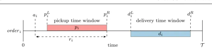
[0,T) is the period in which the fleet of vehicles V has to respond to customer requests. The events,E, represent customer transportation requests. Since we con-sider the purely dynamic PDPTW, all events are revealed between time 0 and timeT. Each eventei ∈ E is defined by the following variables:
ai:= announce time
pi:= [pLi, p R
i ) = pickup time window,p L i < p
R i
di:= [dLi, dRi ) = delivery time window,dLi < dRi psti:= pickup service time span
dsti:= delivery service time span ploci:= pickup location
dloci:= delivery location
tti:= travel time from pickup location to delivery location
Reaction time is defined as:
ri :=pRi −ai= reaction time (1)
The time window related variables of a transportation request are visualized in Figure 1.
Furthermore it is assumed that:
– vehicles start at a depot and have to return after all orders are handled;
– the fleet of vehiclesV is homogeneous;
time
0 T
ri orderi
ai pLi pRi dLi dRi
pickup time window
pi
delivery time window
[image:7.595.73.415.74.152.2]di
Fig. 1: Visualization of the time related variables of a single order eventei∈ E.
– the vehicle is either stationary or driving at a constant speed;
– vehicle diversion is allowed, this means that a vehicle is allowed to divert from its destination at any time;
– vehicle fuel is infinite and driver fatigue is not an issue;
– the scenario is completed when all pickup and deliveries have been made and all vehicles have returned to the depot; and,
– each location can be reached from any other location.
Vehicle schedules are subject to both hard and soft constraints. The opening of time windows is a hard constraint, hence vehicles need to adhere to these:
spij≥pLi (2)
sdij≥dLi (3)
spij is the start of the pickup operation of order eventei by vehiclevj; similarly,
sdij is the start of the delivery operation of order eventeiby vehiclevj. The time window closing (pRi anddRi ) is a soft constraint incorporated into the objective function, it needs to be minimized:
min:=X
j∈V
(vttj+td{bdj,T }) + X
i∈E
td
n
spij, pRi o
+td n
sdij, dRi o
(4)
where
td{α, β}:=max{0, α−β} = tardiness (5) vttj is the total travel time of vehicle vj; bdj is the time at which vehiclevj is back at the depot. In summary, the objective function computes the total vehicle travel time, the tardiness of vehicles returning to the depot and the total pickup and delivery tardiness.
2.2 Dataset
Earlier work has argued for, and presented, a dataset characterized by three dif-ferent properties of dynamic PDPs: dynamism, urgency, and scale [4].
2.2.1 Dynamism
introduces additional information to the problem, such as the events inE. Formally, the degree of dynamism, or the continuity of change, is defined as:
dynamism := 1−
|∆|
X
i=0
σi
|∆|
X
i=0
¯
σi
(6)
∆is the list of event interarrival times:
∆:={δ0, δ1, . . . , δ|E|−2}={aj−ai|j=i+ 1∧ ∀ai, aj∈ E} (7)
The interarrival time for a scenario with 100% dynamism is called the perfect interarrival time:
θ:= perfect interarrival time = T
|E| (8)
Based on this definition, the deviation and maximum possible deviation to the perfect interarrival time can be computed:
σi:=
θ−δi ifi= 0 andδi< θ
θ−δi+
θ−δi
θ ×σi−1 ifi >0 andδi< θ
0 otherwise
(9)
¯
σi:=θ+
θ−δi
θ ×σi−1 ifi >0 andδi< θ
0 otherwise
(10)
eq. 6 uses the proportion of the actual deviation and the maximum possible devia-tion. Using this definition the degree of dynamism of any scenario can be computed.
2.2.2 Urgency
In [3] urgency is defined as the maximum reaction time available to the fleet of vehicles in order to respond to an incoming order. Or more formally:
urgency(ei) :=pRi −ai=ri (11)
To obtain the urgency of an entire scenario the mean and standard deviation of the urgency of all orders can be computed.
2.2.3 Scale
2.3 Realistic simulation platform
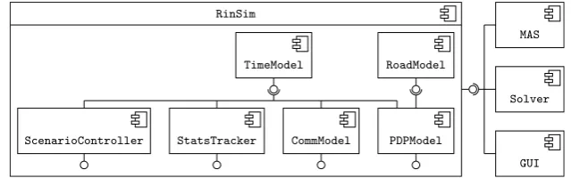
The experiments performed in van Lon and Holvoet [5] use the RinSim real-time logistics simulator [17]. For fair comparison we use the same simulator. RinSim is a discrete-time logistics simulator that supports running both centralized algo-rithms and decentralized multi-agent systems. RinSim is written in Java and has a modular design (Figure 2), a Model encapsulates a part of a problem domain or algorithm. The simulator can be customized by selecting the models that are
TimeModel RoadModel
ScenarioController StatsTracker CommModel PDPModel RinSim
MAS
Solver
[image:9.595.84.404.201.301.2]GUI
Fig. 2: UML component diagram of RinSim. The simulator subsystem can be configured with a variety of models that all provide some interface. MASs, solvers, and the graphical user interface use these interfaces to interact with RinSim.
used, this allows simulating a wide variety of logistics problems while maximally reusing existing code.
RinSim supports simulations using simulated time as well as real-time. The standard Java virtual machine (JVM) has no built-in support for real-time exe-cution. However, RinSim is designed such that it provides soft real-time behavior using the standard JVM. Soft real-time, as opposed to hard real-time, allows oc-casional deviations from the desired execution timing.
RinSim discretizes time into intervals called ‘ticks’. The simulator is initialized with a fixed tick length, for example a tick length of 250 milliseconds. When simulating without real-time constraints, the simulator computes all ticks as fast as possible. In a real-time simulator the interval between the start of two ticks should be the tick length (e.g. 250 ms). Since the JVM doesn’t allow precise control over the timings of threads it is generally impossible to guarantee hard real-time constraints. In real-real-time mode, RinSim uses a dedicated thread for executing the ticks. If computations need to be done that are expected to last longer than a tick, they must be done in a different thread. This minimizes interference of computations with the advancing of time in the simulated world. Additionally, the processor affinity of the threads are set at the operating system level. Setting the processor affinity to a Java thread instructs the operating system to use one processor exclusively for executing that thread. In practice, the actual scheduling of threads on processors depends on the number of available processors and the operating system.
com-putations are being done other than that of the simulator advancing time in the simulated world. For this reason, RinSim employs a mechanism to dynamically switch between real-time and simulated time. When the simulator is in simulated time, ticks will be executed as fast as possible speeding up the simulation signifi-cantly. As soon as a computation needs to be done, the simulator must first switch back to real-time mode before this computation can be started.
3 Multi-agent systems for dynamic PDP
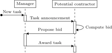
This section is adapted from [5]. The multi-agent system that is extended is an implementation of the dynamic contract-net protocol (DynCNET) presented by Weyns et al. [18]. DynCNET is a dynamic extension of the CNET first proposed by Smith [19]. Inspired by how companies use subcontracting to collaboratively solve problems, CNET uses contracting to approach the task assignment problem. In CNET, the agent that tenders a task is called themanager and it sends a task announcement to potentialcontractors. Each potential contractor can either ignore the announcement or send abidto the manager. The manager then selects its best bid and awards the task to the contractor. Figure 3 shows the UML interaction diagram for the CNET auction process. Although an auction can be, and usually
Manager
New task
Task announcement
Potential contractor
Compute bid Propose bid
[image:10.595.147.339.338.429.2]Award task
Fig. 3: UML interaction diagram of a CNET auction.
is, used in a competitive setting, we use auctions in a purely cooperative setting. We assume that both the contractors and the manager are working for the same company. The dynamic extension of CNET provides flexibility to the assignment until a contractor has to commit to the execution of the task. The same task can be announced several times before its execution, its assignment changing after every announcement.
New task :OrderAgent
Announce
v2:VehicleAgent
Compute :RinSim
Announce
v1:VehicleAgent
Compute
Several ticks Propose bid Done
Several ticks Propose bid Done
opt [Stop criterion]
Finalize auction
Award
[image:11.595.82.417.71.255.2]End of auction
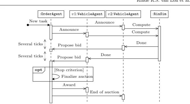
Fig. 4: UML interaction diagram of an auction of an order with two vehicles. Upon receiving the auction announcement, bothVehicleAgents start computing a bid. The computations take several ticks. As soon as theOrderAgenthas met the stop criterion, in this case receiving two bids is enough, the auction is finalized and the order is awarded tov1. Vehiclev2 is notified of the end of the auction. TheRinSim lifeline is a simplified view of the multi-threaded computation facilities provided by RinSim. Note that the filled arrows indicate synchronous calls and the stick arrows indicate asynchronous calls.
order that is to be offered to start a new auction, theOrderAgentwill then perform a new auction process similar to Figure 4. A possible outcome of this auction is that the order is not awarded to another vehicle but stays assigned to the original vehicle. Allowing the vehicles to start a new auction process enables the dynamic (re)allocation of orders and makes the CNET implementation dynamic.
3.1 Order agent
TheOrderAgent(the manager in CNET terminology) is responsible for the auction process. It announces the start of the auction to all vehicles and waits until it receives enough bids to make a decision. The stop criterion for the bidding process is:
|bids| ≥2∧(|bids|=|vehicles| ∨auction duration≥5000)
where, |bids| is the number of received bids, |vehicles| is the total number of vehicles which equals the potential maximum number of bids andauction duration
is the duration of the auction in milliseconds.
their computations. Bids that are received after the finalization of the auction are ignored.
3.2 Vehicle agent
A VehicleAgent needs to compute a bid value in order to propose a bid. In [5] the bid value is computed using a solver. The cost of an order is defined as the additional cost that including that order incurs to a vehicle’s current schedule:
cost(order) =cost(new schedule)−cost(current schedule) (12)
where,current scheduleis the schedule of the vehicle including all previous order assignments, andnew scheduleis the current schedule of the vehicle including the proposed order. The task of the solver is finding the bestnew schedulein a relative short amount of time to get a reliable estimate of the cost of the auctioned order. The time for computing the new schedule is limited because the auction process has a limited duration, the bid needs to be proposed before the end of this duration in order to ensure that theOrderAgentwill take the bid into account.
As soon as the assignment of orders to a vehicle has changed, theVehicleAgent needs to update its schedule. The vehicle’s schedule is optimized by a solver (the schedule solver), although it is imperative to generate acompleteschedule quickly, it is not necessary to limit the duration of the solver as the solver can continu-ously notify theVehicleAgentof improved schedules. This allows the optimization process to continue for an extended period.
The VehicleAgentconsiders starting a new auction in the following two situ-ations:
– when a vehicle hasn’t won an auction for at least five minutes; or,
– when the vehicle’s current schedule has changed.
When starting a new auction the vehicle has to decide which of its previously as-signed orders it should auction. The order that when removed yields the greatest schedule cost reduction is selected. The cost reduction of removing an order does not require an optimization step and can therefore be computed quickly for all orders assigned to a vehicle (similar to eq. 12). Orders for which the pickup opera-tion is in process or is already done are not considered for aucopera-tioning as they can’t be reassigned. If the order with the greatest cost reduction is the last received order, no auction is performed to avoid excessive auctioning. TheVehicleAgent itself has to propose a bid to its own auction, only when another agent proposes a better bid will the order be reassigned.
4 Genetic programming for enhancing agents
4.1 Heuristics in agents
As described in Section 3, theVehicleAgenthas three different decisions to make: 1. Assigning a bid value to an auctioned parcel, currently being done using
cheap-est insertion cost with the insertion computed by OptaPlanner.
2. Deciding what parcel to reauction, currently taking the most expensive parcel. 3. Finding the cheapest route to all destinations, currently computed using
Opta-Planner.
Assigning a bid value to a parcel (1) and deciding which parcel to reauction (2) can easily be done by a heuristic:
(vehicle,parcel) -> cost
The heuristic is executed by a vehicle, the output is an estimation of the cost of adding the specified parcel into the route of the vehicle.
4.2 Genetic programming setup
Since the quality of a heuristic can not analytically be deduced, we are using simulation-based fitness evaluation. Since real-time simulation is very time con-suming, we are using RinSim (Section 2.3) with simulated time during evolution. Additionally, to also save computation time, we use the cheapest insertion cost heuristic instead of OptaPlanner for computing the cheapest route to all destina-tions. To avoid spending too much time on simulating inferior individuals we use RinSim with a custom stop condition:
stop(t) := (
∃vi ∈ Vroute length(vi)>max (40,|Et| − |Dt|) ift≤8 hours
true otherwise
wheret is the current time,|Et|is the number of parcel announce events at time
t, and |Dt| is the number of delivered parcels at time t. The stop condition is designed to stop the simulation if it takes too long to deliver all parcels or if there is a single vehicle that is hoarding parcels. Hoarding is defined as a vehicle that has more than about 50% of parcels in its route. A vehicle route may contain each parcel at maximum twice, if the route length is larger than the number of undelivered parcels this means that about 50% of the parcels are in that route. The stop condition only applies when the total route length is more than 40. The stop condition halts simulations of bad quality individuals, saving computation time for individuals of higher quality.
The fitness function, that needs to be minimized, is:
fitness := (
fitnessmax−t if simulation terminated early cost (eq. 4) otherwise
The fitness of individuals that are stopped by the stop condition is the maximum fitness value subtracted with the time of the simulator at which it was stopped. This adds some differentiation to low quality individuals.
Table 1: Genetic programming settings
Parameter Value
Population size 500
Generations 100
Number of evaluations per individual 50 Num evals in last generation 250
Crossover proportion 90%
Mutation proportion 10%
Elitism 1
Selection method Tournament selection (size 7)
Maximum tree depth 17
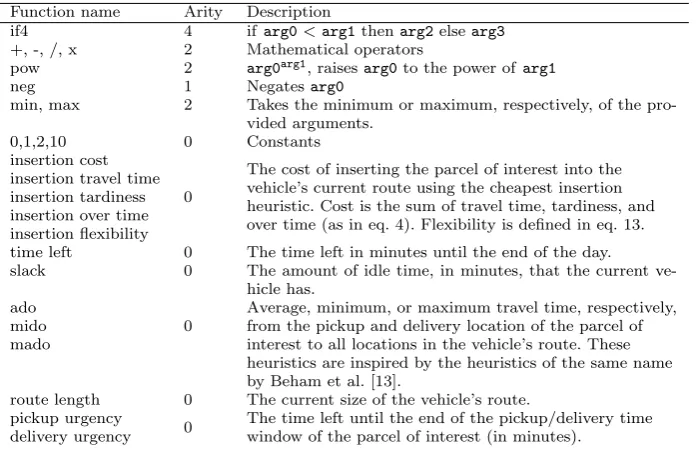
evaluations per individual needs to be high enough to avoid over specialization within a single generation while it needs to be low enough to keep the experiments computationally feasible. Table 2 lists the functions and terminals that are used. One of the variables is based on the concept of flexibility in a route. Flexibility
Table 2: Functions and terminals used in GP. The terminals have a context of a vehicle (the vehicle that executes the heuristic) and a parcel of interest.
Function name Arity Description
if4 4 ifarg0<arg1thenarg2elsearg3
+, -, /, x 2 Mathematical operators
pow 2 arg0arg1, raisesarg0to the power ofarg1
neg 1 Negatesarg0
min, max 2 Takes the minimum or maximum, respectively, of the pro-vided arguments.
0,1,2,10 0 Constants
insertion cost
0
The cost of inserting the parcel of interest into the vehicle’s current route using the cheapest insertion heuristic. Cost is the sum of travel time, tardiness, and over time (as in eq. 4). Flexibility is defined in eq. 13. insertion travel time
insertion tardiness insertion over time insertion flexibility
time left 0 The time left in minutes until the end of the day. slack 0 The amount of idle time, in minutes, that the current
ve-hicle has. ado
0
Average, minimum, or maximum travel time, respectively, from the pickup and delivery location of the parcel of interest to all locations in the vehicle’s route. These heuristics are inspired by the heuristics of the same name by Beham et al. [13].
mido mado
route length 0 The current size of the vehicle’s route. pickup urgency
0 The time left until the end of the pickup/delivery time window of the parcel of interest (in minutes).
delivery urgency
is the degree to which arrival times in a vehicle’s route can be changed without introducing time window violations. This is calculated as follows:
flexibility(route) :=
|route|
X
ri∈route
lpa(ri)−epa(ri) (13)
[image:14.595.73.423.322.550.2]Even though we simulate each individual on 50 different scenarios, the difficulty of scenarios varies. Within a generation this is not a problem because fitness is relative. However, a convergence graph that shows absolute values will show a lot of noise. Therefore, we normalize the fitness values to the cost of the cheapest insertion cost heuristic.
4.3 Tuning
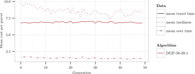
For investigating the performance of GP we ran some experiments with a smaller number of generations. Figure 5 shows a breakdown of the convergence graph of such a run. The figure shows that most of the improvement during evolution
2.5 5.0 7.5 10.0
0 10 20 30 40 50
Generation
Mean
cost
p
e
r
parce
l
Data
mean travel time
mean tardiness
mean over time
Algorithm
[image:15.595.83.408.265.388.2]DGP-50-20-1
Fig. 5: Breakdown of cost per generation of a single evolutionary run on a scenarios with 50% dynamism, 20 minutes urgency and scale 1.
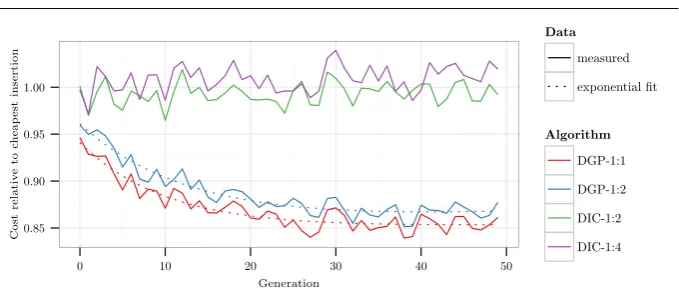
is caused by a reduction of tardiness and over time while travel time remains relatively constant. This suggests that it may be worthwhile to emphasize the tardiness in the objective function during evolution. Figure 6 shows the relative performance of two weighted versions of the cheapest insertion heuristic. From Figure 6 it can be concluded that DIC-1:2 performs better than the 1:1 objective function while DIC-1:4 performs worse than 1:1. However, replacing the insertion based GP variables with weighted versions does not benefit evolution, DGP-1:1 outperforms DGP-1:2. This is presumably because evolution already favors heuris-tics that emphasize reducing tardiness and over time as this yields the greatest performance increase.
5 Evaluation
0.85 0.90 0.95 1.00
0 10 20 30 40 50
Generation
Cost
relativ
e
to
c
heap
est
insertion
Data
measured
exponential fit
Algorithm
DGP-1:1
DGP-1:2
DIC-1:2
[image:16.595.78.418.76.220.2]DIC-1:4
Fig. 6: Comparison of two evolutionary settings (average of three repetitions each), DGP-1:1 with standard objective function weights of its variables defined in Ta-ble 2 and DGP-1:2 with objective functions weights in favor of tardiness and over time. DIC-1:2 and DIC-1:4 are using weighted insertion cost (without evolution) on the same set of scenarios as are used in every generation of the GP.
5.1 Training
For training we have generated a separate dataset using the same settings (but different random seeds) as used in [5]. During training we only use small scale scenarios to save computation time.
5.1.1 Experiment setup
We have opted for four different GP setups (Table 3). Three setups are meant
Table 3: The four different GP setups, DGP-50-20-1, DGP-50-20-1, and DGP-80-5-1 are specialized setups that train on one specific class of scenarios. DGP-mixed is a setup that trains on all small scale scenario classes simultaneously.
Dynamism Urgency Scale Num evals Num last evals Name
20% 35 1
50 250
DGP-20-35-1
50% 20 1 DGP-50-20-1
80% 5 1 DGP-80-5-1
20%/50%/80% 35/20/5 1 54 270 DGP-mixed
to specialize on one specific scenario class, while the DGP-mixed setup aims to generate generalized heuristics that are equally adapted to all scenarios. Because there are nine small scale scenario classes, we use 54, a multiple of nine, evaluations every generation. This ensures that each generation each individual is evaluated on exactly six scenarios of every scenario class.
seconds each on a modern PC. If the average simulation time would be exactly 1 second, the expected total computation time is about 1227 days (3.3 years). Clearly, it is not feasible to run such an experiment on a single computer, there-fore we have pooled the resources of about 80 modern quad-core computers to run our simulations. Theoretically, these 80 machines allows us to perform about 320 simulations in parallel. In practice, however, these are shared university machines that may have other processes running or may simply be turned off during an experiment. To utilize these machines we use a feature of RinSim that allows to spread simulations over multiple machines (internally using JPPF [20]) and that is resistant to single node failures.
5.1.2 Results and analysis
[image:17.595.76.414.333.553.2]A total of 103,374,996 simulations were computed during the course of the 40 evolutionary runs. The cumulative computation time is 1295 days, using the dis-tributed computing setup, it took slightly more than 10 days. The actual number of simulations that were performed is slightly lower because when identical indi-viduals are found within a generation they are evaluated only once.
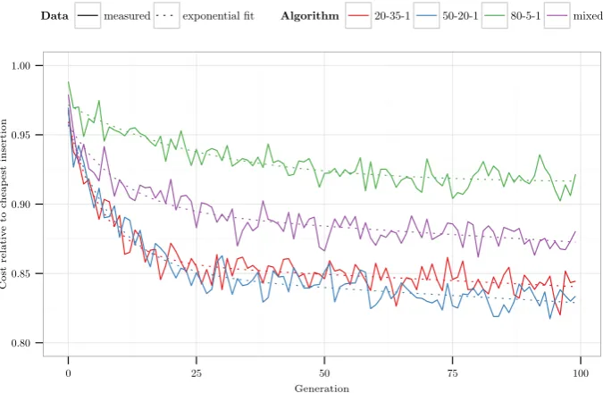
Figure 7 shows the average convergence graphs of each GP variant. For all GP
0.80 0.85 0.90 0.95 1.00
0 25 50 75 100
Generation
Cost
relativ
e
to
c
heap
est
insertion
Data measured exponential fit Algorithm 20-35-1 50-20-1 80-5-1 mixed
Fig. 7: Average convergence graphs based on ten repetitions for each of the four GP settings.
and with an urgency of 5 minutes, each new order needs to be dealt with swiftly. Based on this graph, it appears that the insertion cost heuristic is performing relatively well in these circumstances. For the 20-35-1 and 50-20-1 settings, GP seems to be able to find the largest improvement relative to the insertion cost heuristic. GP-mixed uses all scenario classes and lies, as expected, somewhere between the others.
5.2 Testing
In order to evaluate the effectiveness of our GP approach, we test the evolved heuristics using real-time RinSim [17] on the same dataset as was used in [5].
5.2.1 Experiment setup
The test dataset has three levels of dynamism, urgency, and scale, resulting in 27 different scenarios classes. For each class, the dataset contains ten scenario instances. The evolutionary runs (Section 5.1) produced 40 heuristics, additionally we are also testing the insertion cost heuristic. This means we have 41 algorithms, each of whom we need to test in real-time on the 270 different scenarios in the dataset, resulting in a total of 11,070 real-time simulations. Unlike [5], we do not repeat the execution of simulations with exactly the same settings. Instead, we combine the results of the ten heuristics evolved with the same GP settings and compare those with the results of [5].
To allow direct comparison of the results, we use the same hard- and software as in [5]. The test computer has 24 logical cores (two six core Intel Xeon 2.6GHz E5-2630 v2 processors with hyper threading). A single simulation requires two logical cores, one for the simulator and one for the solver computations. At least one core needs to be available for the operating system, resulting in a maximum of 11 simulations that can be run in parallel. As in [5], we warm up the JVM for 30 seconds before starting the real-time experiment.
5.2.2 Results
The following section reports on the 60% of the results that have been completed so far1. Table 4 lists the algorithms that we compare. Similar to [5], we apply Welch’st-test for testing the significance of the differences between the algorithms. In the following analysis we refer to this test by mentioning the p-values (when relevant) that were observed. The significance threshold was set at p = .01. For pairs of algorithms that have the same number of simulations we perform a paired
t-test instead of an unpairedt-test. The experiment computation time of the 6750 simulations was about 341.5 hours (14.2 days). Table 5 shows all simulation results.
1 Due to the significant computational demands of real-time simulations, only six of the ten
Table 4: Algorithm names with their meaning and number of simulations per class that were performed. For COP and DOP, three repetitions were done for each of the ten scenarios in a class. For the rest of the algorithms, no repetitions were done. For the DGP variants, each of the six evolved heuristics were simulated on each scenario.
Algorithm Description Simulations per class
COP Centralized OptaPlanner (from [5]) 30
DOP Decentralized OptaPlanner (from [5]) 30
DIC Decentralized insertion cost 10
agen
ts
with
genetic
programming
[image:20.595.193.766.129.415.2]19
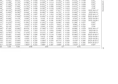
Table 5: Average results for each setting. The ‘Best’ column indicates which algorithms has the best performance, the rank of each value is indicated by the number in superscript, a†appended to a value with ranknindicates that the difference between the value of ranknand rankn+ 1 is not statistically significant (p <0.01). The results of the four evolved algorithms also report their standard deviation as the numbers are the average of the different heuristics produced by GP.
Class COP DOP DIC DGP-20-35-1 DGP-50-20-1 DGP-80-5-1 DGP-mixed Best
20-5-1 25.0131† 26.9135† 27.0426† 27.3887 ± 1.166 26.2914† ± 1.087 25.6222†± 0.558 25.7293†± 0.425 COP†
50-5-1 22.1123 22.8894† 23.2186† 23.9347 ± 1.762 23.1345† ± 1.242 21.4901†± 0.335 21.8982†± 0.422 DGP-80-5-1†
80-5-1 21.3932† 21.8224† 22.7826† 23.9007 ± 1.897 22.7715† ± 1.050 21.3321†± 0.358 21.7013†± 0.240 DGP-80-5-1† 20-20-1 17.3271† 20.0496† 20.7487 18.8453†± 0.333 18.7972† ± 0.315 19.1975†± 0.378 18.8704†± 0.362 COP†
50-20-1 14.9681† 15.8256† 16.8787 15.2503†± 0.440 15.2132† ± 0.260 15.5855†± 0.647 15.2784†± 0.308 COP†
80-20-1 14.5341† 15.5996 17.7507 14.9664†± 0.393 14.8303† ± 0.114 15.3795†± 0.453 14.8232†± 0.188 COP†
20-35-1 14.6661† 17.3926† 18.7487 16.4793†± 0.487 16.2612† ± 0.245 16.9845†± 0.919 16.5324†± 0.269 COP†
50-35-1 13.0161 15.6896† 17.6367 14.7034†± 0.278 14.6323† ± 0.368 14.9435†± 0.448 14.6142†± 0.302 COP 80-35-1 12.5081 14.2536 16.3037 13.8804†± 0.226 13.5952† ± 0.193 14.2055†± 0.612 13.8123†± 0.321 COP
20-5-5 18.8133† 20.1635† 20.2296† 20.6577 ± 3.448 19.5224† ± 3.087 17.8171†± 0.253 17.9772†± 0.334 DGP-80-5-1†
50-5-5 17.0295 15.6033† 18.5906† 18.8047 ± 4.652 16.2804† ± 2.056 14.7551 ± 0.115 15.0022†± 0.319 DGP-80-5-1
80-5-5 17.1645† 15.4413 18.5497 18.4506†± 3.937 16.1274 ± 1.912 14.7001†± 0.169 14.8602 ± 0.252 DGP-80-5-1†
20-20-5 14.0824† 17.8757 17.6566† 13.9342†± 0.414 13.8561† ± 0.133 14.7485†± 0.724 14.0433†± 0.307 DGP-50-20-1† 50-20-5 10.1294† 10.8826 14.1767 9.8363†± 0.134 9.5101 ± 0.119 10.2575†± 0.702 9.7642†± 0.139 DGP-50-20-1
80-20-5 10.3504† 10.7876 14.8517 10.2183†± 0.182 9.8601 ± 0.190 10.4855†± 0.721 10.0942†± 0.216 DGP-50-20-1
20-35-5 11.0151† 15.2726† 15.5557 11.0912†± 0.250 11.2353† ± 0.161 12.0655 ± 0.645 11.2964 ± 0.277 COP†
50-35-5 8.6511† 10.7316 14.4437 8.9192†± 0.273 8.9683†± 0.274 9.8215 ± 0.707 9.0684 ± 0.223 COP†
80-35-5 8.7841 10.1436 14.8177 9.1672†± 0.294 9.2834 ± 0.224 9.9535† ± 0.657 9.2633†± 0.242 COP 20-5-10 17.4883† 27.4307 18.9265† 20.0736 ± 6.252 17.5894† ± 3.317 15.9041†± 0.137 16.0082 ± 0.379 DGP-80-5-1†
50-5-10 15.5584 15.9585 17.5176† 18.0417 ± 7.223 14.1153 ± 2.010 12.8081 ± 0.168 12.9652 ± 0.370 DGP-80-5-1
80-5-10 15.7625† 13.7653† 17.7837 17.4546†± 5.618 14.3154 ± 2.007 12.8871 ± 0.162 13.0872 ± 0.424 DGP-80-5-1
20-20-10 11.4474† 23.8257 15.0436 10.7862†± 0.286 10.7691† ± 0.144 11.6365 ± 0.733 10.9663†± 0.238 DGP-50-20-1†
50-20-10 9.3184† 13.2626 14.2607 8.9283 ± 0.221 8.6131 ± 0.066 9.4285 ± 0.779 8.8382†± 0.183 DGP-50-20-1
80-20-10 9.1924† 10.5146 14.1497 8.8433 ± 0.214 8.5071 ± 0.140 9.2595 ± 0.701 8.7412†± 0.153 DGP-50-20-1
20-35-10 9.7724† 23.4417 13.9836 9.1381†± 0.259 9.4062†± 0.279 10.1715 ± 0.623 9.4193†± 0.300 DGP-20-35-1†
50-35-10 7.9182† 15.5607 14.0046 7.9021†± 0.229 8.0603†± 0.451 8.8185 ± 0.749 8.0824 ± 0.260 DGP-20-35-1†
80-35-10 7.8011† 12.5486 14.0787 7.8022†± 0.212 7.9984 ± 0.407 8.6605 ± 0.724 7.9183†± 0.247 COP†
5.3 Analysis
[image:21.595.87.407.213.271.2]The first hypothesis (Section 1) states that hyper-heuristics (DGP) can outper-form DOP. We can accept this hypothesis as the results indicate that there is always at least one of the DGP variants that outperform DOP (Table 6). In fact,
Table 6: Summary of relative performance of DGP variants to DOP. Each number indicates the number of classes on which the algorithm is (sign.) better or worse compared to DOP.
Algorithm sign. better better (not sign.) worse (not sign.) sign. worse
DIC 4 1 9 13
DGP-20-35-1 13 6 0 8
DGP-50-20-1 15 7 4 1
DGP-80-5-1 16 11 0 0
DGP-mixed 18 9 0 0
DGP-mixed and DGP-80-5-1 are better than DOP for all scenario classes. How-ever, for small scale scenarios the differences between DGP-mixed and DOP and between DGP-80-5-1 and DOP are often not significant. This indicates that the evolved heuristics perform relatively better on larger scale scenarios. This is in-teresting because the heuristics were never trained on large scale scenarios. It appears that the evolved heuristic is more scalable than the OptaPlanner algo-rithm used in DOP. The scalability of the evolved heuristic can likely be explained by its computational efficiency relative to that of OptaPlanner. Table 6 shows investigate
further: compare runtimes of Opta-Planner and heuristic inside agent investigate further: compare runtimes of Opta-Planner and heuristic inside agent
that DGP-20-35-1 and DGP-50-20-1 often outperform DOP but not as often as DGP-80-5-1 and DGP-mixed. DGP-20-35-1 and DGP-50-20-1 have the tendency to perform relatively better on larger scale scenarios. It’s also noteworthy that DIC outperforms DOP in several classes, indicating that in some cases even a simple heuristic can be better than OptaPlanner.
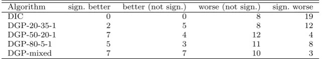
The second hypothesis states that DGP can outperform COP. This hypothesis can be accepted since the evolved heuristics regularly outperform COP (Table 7). However, COP still performs best in 12 of the 27 classes. The scale and urgency
Table 7: Summary of relative performance of DGP variants to COP. Each number indicates the number of classes on which the algorithm is (significantly) better or worse compared to COP.
Algorithm sign. better better (not sign.) worse (not sign.) sign. worse
DIC 0 0 8 19
DGP-20-35-1 2 5 8 12
DGP-50-20-1 7 4 12 4
DGP-80-5-1 5 3 11 8
DGP-mixed 7 7 10 3
[image:21.595.85.410.539.598.2]The third hypothesis states that the evolved heuristics perform especially well in more urgent circumstances. Based on Table 5 it is clear that evolved heuristics outperform COP in eight of the nine very urgent classes (urgency of five minutes), we can therefore accept this hypothesis. The class where COP is better than the evolved heuristics is 20-5-1. In this class, COP is not significantly different from DGP-80-5-1 (p≈.43), DGP-mixed (p≈.35), and DGP-50-20-1 (p≈.10).
[image:22.595.107.385.329.371.2]Hypothesis four states that specialized heuristics outperform general heuristics on scenarios for which they are specialized. DGP-20-35-1 outperforms DGP-mixed on class 20-35-1, however, DGP-50-20-1 performs best of the evolved heuristics on this class. DGP-50-20-1 performs best on its training class, 50-20-1, as does DGP-80-5-1 on 80-5-1. So, for all three classes on which was trained explicitly the specialized heuristic outperforms the general heuristic, we therefore accept the hypothesis. The urgency on which a heuristic was trained is a strong indicator of how well it will perform on a scenario class, therefore, we created a summary of the relative performance of the DGP variants, grouped by urgency (Table 8).
Table 8: Summary of relative performance of DGP variants per urgency level. Each number indicates the number of classes on which the algorithm is the best DGP approach for that urgency level.
Urgency DGP-20-35-1 DGP-50-20-1 DGP-80-5-1 DGP-mixed
5 0 0 9 0
20 0 8 0 1
35 6 2 0 1
The fifth hypothesis states that generalized heuristics outperform specialized heuristics on scenarios for which they are not specialized. Based on Table 8 we can reject this hypothesis. There are only two classes, 80-20-1 and 50-35-1, where DGP-mixed outperforms the other evolved heuristics. Nevertheless, the DGP-mixed method produces heuristics of a good quality as is demonstrated by its average rank of 2.67 which is second best, only COP has a better average rank.
As expected, DIC is on average the worst performing algorithm. There are, however, several cases where DGP-20-35-1 performs worse compared to DIC. The data in Table 5 shows that DGP-20-35-1 performs among the worst in the most urgent scenarios. This is expected considering that it was trained on the least urgent scenarios. The results of this heuristic are made even worse by one heuristic that performs especially bad (as can be seen by the larger than usual standard deviations). When removing this badly performing heuristic from the analysis, the ranks for the DGP-20-35-1 are still among the worst for the very urgent classes. This indicates that the bad performance is not just explained by this one outlier.
6 Conclusion
agent-based hyper-heuristic approach on a real-time logistics problem that sys-tematically varies the dynamism, urgency, and scale of the problem. The results show that our hyper-heuristic outperforms a reference algorithm in all scenar-ios. Additionally, the decentralized hyper-heuristic approach even outperforms the centralized reference algorithm in most situations. The hyper-heuristic approach performs relatively better on more urgent and larger scale problems. The hyper-heuristic approach has the additional advantage that it can specialize on certain problem characteristics, increasing its performance even further.
Acknowledgements This research is partially funded by the Research Fund KU Leuven.
References
1. Sophie N. Parragh, Karl F. Doerner, and Richard F. Hartl. A survey on pickup and delivery problems. Part II: Transportation between pickup and delivery locations. 58(2):81–117, 2008.
2. Gerardo Berbeglia, Jean-Fran¸cois Cordeau, and Gilbert Laporte. Dynamic pickup and delivery problems.European Journal of Operational Research, 202 (1):8–15, 2010. ISSN 03772217. doi:10.1016/j.ejor.2009.04.024.
3. Rinde R. S. van Lon, Eliseo Ferrante, Ali E. Turgut, Tom Wenseleers, Greet Vanden Berghe, and Tom Holvoet. Measures of dynamism and ur-gency in logistics. European Journal of Operational Research, 253(3):614–624, 2016. ISSN 0377-2217. doi:10.1016/j.ejor.2016.03.021.
4. Rinde R. S. van Lon and Tom Holvoet. Towards systematic evaluation of multi-agent systems in large scale and dynamic logistics. In Qingliang Chen, Paolo Torroni, Serena Villata, Jane Hsu, and Andrea Omicini, editors,PRIMA 2015: Principles and Practice of Multi-Agent Systems: 18th International Con-ference, Bertinoro, Italy, October 26-30, 2015, Proceedings, pages 248–264. Springer International Publishing, Cham, 2015. ISBN 978-3-319-25524-8. doi:10.1007/978-3-319-25524-8 16.
5. Rinde R. S. van Lon and Tom Holvoet. When do agents outperform centralized algorithms? A systematic empirical evaluation in logistics.Autonomous Agents and Multi-Agent Systems, 2016. under review.
6. Geoffrey De Smet et al. OptaPlanner User Guide. Red Hat and the com-munity. URLhttp://www.optaplanner.org. OptaPlanner is an open source constraint satisfaction solver in Java.
7. Edmund K Burke, Michel Gendreau, Matthew Hyde, Graham Kendall, Gabriela Ochoa, Ender ¨Ozcan, and Rong Qu. Hyper-heuristics: a survey of the state of the art. Journal of the Operational Research Society, 64(12): 1695–1724, jul 2013. ISSN 0160-5682. doi:10.1057/jors.2013.71.
8. Edmund K. Burke, Matthew Hyde, Graham Kendall, Gabriela Ochoa, En-der ¨Ozcan, and John R. Woodward. A Classification of Hyper-heuristic Ap-proaches, pages 449–468. Springer US, Boston, MA, 2010. ISBN 978-1-4419-1665-5. doi:10.1007/978-1-4419-1665-5 15.
10. J. Branke, S. Nguyen, C. W. Pickardt, and M. Zhang. Automated de-sign of production scheduling heuristics: A review. IEEE Transactions on Evolutionary Computation, 20(1):110–124, Feb 2016. ISSN 1089-778X. doi:10.1109/TEVC.2015.2429314.
11. Robert E. Keller and Riccardo Poli. Cost-Benefit Investigation of a Genetic-Programming Hyperheuristic, pages 13–24. Springer Berlin Heidelberg, Berlin, Heidelberg, 2008. ISBN 978-3-540-79305-2. doi:10.1007/978-3-540-79305-2 2. 12. E. K. Burke, M. R. Hyde, and G. Kendall. Evolving Bin Packing Heuristics with Genetic Programming, pages 860–869. Springer Berlin Heidelberg, Berlin, Heidelberg, 2006. ISBN 978-3-540-38991-0. doi:10.1007/11844297 87.
13. Andreas Beham, Monika Kofler, Stefan Wagner, and Michael Affenzeller. Agent-Based Simulation of Dispatching Rules in Dynamic Pickup and Deliv-ery Problems. 2009 2nd International Symposium on Logistics and Industrial Informatics, pages 1–6, sep 2009. doi:10.1109/LINDI.2009.5258763.
14. Rinde R. S. van Lon, Tom Holvoet, Greet Vanden Berghe, Tom Wenseleers, and Juergen Branke. Evolutionary Synthesis of Multi-Agent Systems for Dynamic Dial-a-Ride Problems. In GECCO Companion ’12 Proceedings of the fourteenth international conference on Genetic and evolutionary compu-tation conference companion, pages 331–336, Philadelphia, USA, 2012. ISBN 9781450311786. doi:10.1145/2330784.2330832.
15. Stefan Vonolfen, Andreas Beham, Michael Kommenda, and Michael Affen-zeller. Structural Synthesis of Dispatching Rules for Dynamic Dial-a-Ride Problems, pages 276–283. Springer Berlin Heidelberg, Berlin, Heidelberg, 2013. ISBN 978-3-642-53856-8. doi:10.1007/978-3-642-53856-8 35.
16. Jonathan Merlevede, Rinde R.S. van Lon, and Tom Holvoet. Neuroevolution of a multi-agent system for the dynamic pickup and delivery problem. In International Joint Workshop on Optimisation in Multi-Agent Systems and Distributed Constraint Reasoning (OptMAS, co-located with AAMAS), 2014. 17. Rinde R. S. van Lon and Tom Holvoet. RinSim: A simulator for collective
adaptive systems in transportation and logistics. In Proceedings of the 6th IEEE International Conference on Self-Adaptive and Self-Organizing Systems (SASO 2012), pages 231–232, Lyon, France, 2012. doi:10.1109/SASO.2012.41. 18. Danny Weyns, Nelis Bouck´e, Tom Holvoet, and Bart Demarsin. DynCNET: A protocol for dynamic task assignment in multiagent systems. First Interna-tional Conference on Self-Adaptive and Self-Organizing Systems, SASO 2007, pages 281–284, 2007. doi:10.1109/SASO.2007.20.
19. Reid G. Smith. The contract net protocol: High-level communication and con-trol in a distributed problem solver.IEEE Transactions on Computers, 29(12): 1104–1113, December 1980. ISSN 0018-9340. doi:10.1109/TC.1980.1675516. 20. Laurent Cohen. Jppf, the open source grid computing solution. URLhttp: