Maximum Entropy Empirical Likelihood Methods Based on Bivariate Laplace Transforms and Moment Generating Functions

(1)

http://www.scirp.org/journal/ojs ISSN Online: 2161-7198

ISSN Print: 2161-718X

DOI: 10.4236/ojs.2018.82017 Apr. 10, 2018 264 Open Journal of Statistics

Maximum Entropy Empirical Likelihood

Methods Based on Bivariate Laplace

Transforms and Moment Generating Functions

Andrew Luong

École d’Actuariat, Université Laval, Québec, Canada

Abstract

Maximum Entropy Empirical Likelihood (MEEL) methods are extended to bivariate distributions with closed form expressions for their bivariate Laplace transforms (BLT) or moment generating functions (BMGF) without closed form expressions for their bivariate density functions which make the implementation of the likelihood methods difficult. These distributions are often encountered in joint modeling in actuarial science and finance. Moment conditions to implement MEEL methods are given and a bivariate Laplace transform power mixture (BLTPM) is also introduced, the new operator generalizes the existing univariate one in the literature. Many new bivariate distributions including infinitely divisible(ID) distributions with closed form expressions for their BLT can be created using this operator and MEEL methods can also be applied to these bivariate distributions.

Keywords

Bivariate Power Mixture Operator, Laplace Transform Copulas, Chi-Square Test Statistics, Bivariate Normality, Infinite Divisibility, Empirical Likelihood

1. Introduction

Bivariate distributions are useful for joint modelling and naturally fitting these distributions is a necessity for pricing in insurance and finance. For example, in finance fitting a bivariate jump diffusion model to joint returns data allowed us to price a basket option accordingly, see Ruijter and Oosterlee [1] (p. B658) for a bivariate jump diffusion model. The authors advocated a two dimensions cosine method for pricing basket option. In actuarial sciences, one might consider modeling two claim amounts from an accident, i.e., the amount from body

How to cite this paper: Luong, A. (2018) Maximum Entropy Empirical Likelihood Methods Based on Bivariate Laplace Trans-forms and Moment Generating Functions. Open Journal of Statistics, 8, 264-283.

https://doi.org/10.4236/ojs.2018.82017

Received: February 14, 2018 Accepted: April 7, 2018 Published: April 10, 2018

http://creativecommons.org/licenses/by/4.0/

(2)

DOI: 10.4236/ojs.2018.82017 265 Open Journal of Statistics

damage and the amount from material damage which are incurred simultaneously in a car accident, see Partrat [2] (p. 225). Joint survival analysis is also useful for lifetime study, see Crowder [3] (pp. 121-136).

In order to find suitable bivariate parametric models, compound methods and copulas are often used. New bivariate distributions created using the traditional distribution or survival copulas are often continuous with closed form distribu-tion funcdistribu-tions or density funcdistribu-tions so that methods based on likelihood funcdistribu-tions can be applied for statistical inferences. It is also well known that many useful bivariate infinitely divisible distributions do not have closed form density function nor distribution function yet very useful for applications.

For the univariate case, the LT power mixture (LTPM) operator as introduced by Abate and Whitt [4] (pp. 92-93) for the univariate set up for creating new distri-bution using Laplace transforms (LT) can be used to generate many distridistri-butions with closed form LT. Furthermore, it can also be used to generate distribution which is infinitely divisible. In this paper we shall generalize the LTPM to a bivariate version, the BLTPM operator and show that the BLTPM operator can be used to generate new bivariate distributions with closed from BLT. Furthermore, the traditional survival copulas such as the Clayton copula, see Shih and Louis [5]

can be used as a LT copula if the property of complete monotonicity of two specific related functions are satisfied. For another class of survival copulas, see Crowder [3]

(pp. 121-138). Consequently, some distribution or survival function copulas which are defined using a generator based on a LT of a nonnegative random variable can be used to generate new distribution with prescribed marginals specified by their marginal LTs. A similar bivariate PM operator based on distribution functions or survival functions, the BDSPM operator has been introduced by Marshall and Olkin [6] (pp. 834-836) to create new distributions functions and with frailty induced distributions, it also related to a class of distribution or survival Copula functions defined with a generator. The BLTPM operator can be used to generate bivariate infinite divisible distributions with closed form BLTs. It appears to be useful to have bivariate infinite divisible distributions for joint modeling as they are related to corresponding bivariate Lévy processes with stationary and inde-pendent increments. These types of processes are useful as they often lead to elegant results in risk theory in actuarial sciences and in finance.

(3)

conditions which can be identified with elements of a basis where the true score functions are projected as in the univariate set up, see Luong [7] (pp. 463-465); these moment conditions which define elements of the base can be extracted from the model BLT or BMGF.

It is also worth to mention that many bivariate distributions with a singular component in a domain such as the Bivariate exponential distribution as intro-duced by Marshall and Olkin [8] (p. 36) or bivariate phase type distribution as given by Assaf et al. [9] (p. 692) do have a closed form bivariate LT so that model testing for these distributions with singular components in the domain can be handled by bivariate MEEL methods. This motivates us to extend MEEL methods to bivariate distributions and the paper is organized as follows.

In Section 2 some examples from actuarial science and finance are given to il-lustrate the usefulness of bivariate models without closed form density functions but with closed form BLTs. The BLTPM operator is introduced in Section 3 and it is shown that it can be used to create bivariate ID distribution with closed form BLT.MEEL methods are introduced in Section 3 with the proposal of two bases to generate moment conditions. The elements of the bases are based or BLT or BMGF and do not need the density functions explicitly. These bases are proposed to balance efficiencies and numerical tractability as a base with a large number of elements tend to create numerical difficulties on implementation of the MEEL methods. The asymptotic properties which already appear in the literature are restated emphasizing bases and projections of the score functions. We also discuss numerical implementation of the MEEL methods using penalty function ap-proach as given by Luong [7]. Section 5 illustrates the use of the methods by conducting a limited simulation study with a bivariate compound Poisson model as proposed by Partrat [2] (pp. 220-223). With the range of parameters as con-sidered, we observe that the MEEL estimators are two to four time more efficient than MM estimators and at the same time provide a chi-square goodness of fit test statistics for model selection. A base of nine elements is chosen in the study and there is no major numerical difficulty encountered on implementation using the penalty function approach. The methods avoid the use of the covariance matrix of the elements of the base as required for the optimum generalized moment methods (GMM) as discussed in Luong [7], the expressions for this optimum covariance matrix can be complicated.

In the next section, we shall give some examples to illustrate that in many situations we end up working with bivariate distributions with closed form BLT or closed from BMGF but without a closed form for distributions functions or den-sity functions.

2. Some Examples

Example 1

(4)

a mass assigned to it. It can be created from compounding using a bivariate Poisson distribution and has closed form BLT and suitable for modelling two claim amounts from two types of claim in actuarial sciences. The vector of claim amount will have two components and each component can be expressed as a random sum as in the univariate case but the two components will be correlated due to the two numbers of claims given by the vector N=

(

N N1, 2

)

′ are dependent

and follow a bivariate Poisson distribution. More precisely, the claim amount is a vector X =

(

Y Z,

)

′. Each of the components of X can be expressed each as a

ran-dom sum. Note that 1

1

N i i

Y=

∑

₌U , the random variables

{

U i_i, =1, 2,

}

are

in-dependent and identically distributed as U≥0 which is a nonnegative

con-tinuous random variable with LT, LU

( )

s . Similarly,

1

N i i

Z=

∑

₌V , the random

variables

{

V i_i, =1, 2,

}

are independent and identically distributed as V ≥0

which is a nonnegative continuous random variable with LT, L tV

( )

. The random variables

{

U i_i, =1, 2,

}

,

{

V i_i, =1, 2,

}

,

{

N N₁, ₂

}

are assumed to be independent and with other related independence assumptions as given by H1-H7 in Partrat [2] (pp. 220-221) leads to the BLT of the vector X expressible as

( )

,

(

U

( ) ( )

, V

)

LX s t =g L s L t , see Partrat [2] (p. 221).

The bivariate probability generating function (BPGF) for N=

(

N N1, 2

)

′ is

denoted by

g s t

( )

,

and if N=

(

N N₁, ₂

)

′ follows a bivariate Poisson distribution

then its PGFis given as _{g s t}

( )

_, =_eф1( )s− +1 ф2( )t− +1 ф12(st−1), see Partrat [2] (p. 222).

The parameters ф ,ф ,ф1 2 12 are all nonnegative. This is the only bivariate

Poisson distribution which is infintely divisble(ID), see Dwass and Teicher [10]. Now if U and V are also ID then with property of the bivariate Poisson PGF, it can be seen that

( ) ( )

(

)

1

, n

U V

g L s L t

 

 

is a BLT for each positive integer n, using the remarks given by Abate and Whitt [4]

based on results given by Feller [11] (p. 176, 449). Consequently, we can conclude that X is also ID. As BLT is closely related to BMGF, a similar conclusion can be made using BMGF instead of BLT. Also In many circumsstances by inspecting the BLT or BMGF which has a closed form expression, we can infer the property of infinitely divisibility of the distribution without having to use more sophisticated methods such as the one based on the Lévy-Khintchine representation, see Dwass and Teicher [10] for this representation which is general but very technical to characterize ID distribution and Lévy process.

Clearly, we can differentiate

L

_X

( )

s t

,

or using a conditioning argument with

the random sums representations to obtain the first two moments of the vector X

and these first two moments will be icluded in the set of moment conditions for MEEL methods developed subsequently in section 4. The following example gives a model which is used in finance.

Example 2

(5)

assets in a period of time. The return random vector is X=

(

Y Z,

)

′ and is

representable as

1

N i i=

= +

∑

X B J ,

with B following a bivariate normal distribution,

B

~

N

(

µ

,

Σ

)

.

The mean vector µ=

(

µ µ ′1, 2

)

and the covariance matrix

11 12

12 22

σ





= 







Σ

_{, the}

random vector B is independent of the random sum 1

N i i=

∑

J , the Ji ’s are independent and identically dsitributed as J which follows a bivariate normal distribution, J~N

(

µ

J,ΣJ

)

with

(

)

11 12

1 2

12 22

, ,

J J

σ σ

µ µ

σ σ

 

′

= _{= } 

 

J _ΣJ

µ

This is a jump-diffusion model with the diffusion part given by B and the jump part by the random sum 1

N i i=

∑

J . Also, the J_i’s, B, Z and N are independent with

N following a Poisson distribution with parameter λ. Comparing to a bivariate normal model, the bivariate jump diffusion model has an extra jump component. Ruijter and Oosterlee [1] (p. B658) show that by letting s=

( )

s t, ′, the BMGF for

W is given by

( )

_, _e 12 _exp _e 12 ₁ _, _,

J J

M s t = ′ + ′ _λ_ ′ + ′ − __ − ∞ <s t< ∞

 

⋅

s s s s s s

X

Σ Σ

µ µ

.

The domain of M_X

( )

s t, is the entire plane due to the use of the Poisson and

normal distributions. Clearly, this an ID BMGF and the corresponding jump diffusion process is a bivariate Lévy process. Also, the first two moments of the vector X can be extracted from the BMGF. For this model, MEEL methods can be used for estimation and model testing. The class of bivariate normal mean variance mixture as described by McNeil et al [12] (pp. 77-78) is another example where bivariate MEEL methods might be suitable.

Furthermore, MEEL methods can also be used for testing the null composite hypothesis which specifies that the parametric model fits the data. The test statistics based on MEEL methods can be constructed in a unified way and obtained simultaneously with the estimation procedures. This feature is useful for doing applied works and the test statistics is less complicated than statistics based on the Mahanolobis distance, see Mc Assey [13], Muldhokar et al. [14] for statistics based on such a distance. The unique asymptotic chi-square distribution that the statistics follows across the composite hypothesis make them suitable statistics to replace the traditional chi-square test statistics as proposed by Moore and Stubblebine [15] which require closed form bivariate density functions. Model testing procedure is easy to implement if it is based on a statistics with a unique asymptotic distribution for all β0∈Ω, the parameter space is

(6)

These properties of bivariate MEEL methods are similar to properties of univariate MEEL methods as discussed by Luong [7] and will be further discussed in section 4. Note that asymptotic theory for empirical likelihood methods as developed by Qin and Lawless [16] (p302-308) is not restricted to univariate distribution and the same can be said for the maximum entropy version. In fact, asymptotic theory for empirical likelihoods is well established for model with multivariate observations which are independent and identically distributed using a set of fixed moment conditions. The example 2 as given by Qin and Lawless [16]

(pp. 311-312) is an example of the use of empirical likelihood methods for a bivariate model. In practice, we would like to choose the moment conditions so that high efficiencies can be achieved and handle the procedures numerically. We focus on these points for a class of distributions with closed form BLT or BMGF and do not emphasize asymptotic theory in the paper.

3. Distributions Created Using the BLTPM Operator

3.1. The BLTPM Operator

(7)

survival functions instead of LTs given by Marshall and Olkin [6] (p. 835), we shall use the acronym BDSPM for this operator.

For illustrations, some examples of new bivariate distribution specified by BLT and created using the BLTPM operator will be given for illustrations in section 3.2. The BLTPM operator can also be used to create new distribution with one mar-ginal distribution which is discrete and the other marmar-ginal being continuous. These types of bivariate distributions appear to be useful for actuarial science and possibly for other fields as well.

Often, we need to know whether a function can be considered as LT of some univariate random variable, the notion of completely monotonicity of a function is useful for characterizing a function to be a proper LT of a random variable and can be found in Feller [11] (pp. 439-440) but it is reproduced here for completeness as Definition and Theorem below.

Definition

A function

ф

( )

s

with the domain given by s≥0 is completely monotone (CM)

if it possesses derivatives ф( )n

of all order and

( )

−1nф( )n

( )

s ≥0.

Theorem

A function

ф

( )

s

with the domain given by s≥0 is the LT of a random

vari-able if and only if it is CM.

Now if we assume that the LT of a random variable 𝑋𝑋is _{f s}ˆ

( )

_{so that} _fˆα

( )

_s _is

a proper LT, also suppose that the LT of another random variable Y is

g t

ˆ

( )

so

that gˆα

( )

t is a proper LT and α is a non-negative random variable with distri-bution function H and LT _{h u}ˆ

( )

_{. Furthermore, we assume that conditioning on a}

realized value α, the LT _fˆα

( )

_s _{which is the LT of a random variable denoted by}

( )

X α and the LT gˆα

( )

t which is the LT of a random variable denoted by Y( )α are independent but when integrate out with respect to the distribution of α will give a new bivariate LT for a vector X=

(

Y Z,

)

′,

( )

, ₀ ˆ

( )

gˆ

( ) ( )

d .

LX s t =

∫

∞fα s ⋅ α t H

α

(1)

Using the LT of α, it can be re-expressed as

( )

_, ˆ

(

_{log ˆ}

( )

_log

(

_ˆ

( )

)

_.

L_X s t =h − f s − g t (2)

Expression (2) gives a definition of the BLTPM operator and it generalizes ex-pression (6.1) given by Abate and Whitt [4] (p. 92) for the univariate LTPM op-erator. Similarly, if MGFs are used instead and they are given respectively by

_{( )}

M

f s , gM

( )

t and hM

( )

u , a new bivariate distribution with BMGF can be created similarly.

( )

_,

(

_log

(

_{( )}

)

_log

(

_{( )}

)

_.

X M M M

M s t =h f s + g t

(3) Observe that if X( )α ,Y( )α are ID and α ≥0 is continuous and ID then the new

(8)

univariate case given by Abate and Whitt [4] (p. 92).

A form of bivariate PM operator, the BSDPM has been used in the literature but with the use of distribution functions or survival functions, see the seminal works of Marshall and Olkin [6] and a class of survival or distribution copula functions are also obtained. This class is defined using a generator which is based on the LT of some nonnegative random variable which forms a subclass of the Archimedean class and will be further discussed in section 3.2. Due to the analogy between the BLTPM operator and BDSPM operator, these distribution or survival copula functions subject to some conditions are also LT copulas. For the Archimedean class, see Klugman et al. [17] (pp. 187-213).

In section 3.2, we shall see that additional requirements are needed when working with LT’s instead of distribution functions or survival functions for the use of these copulas traditionally used to create new bivariate distribution func-tion using prescribed marginal distribufunc-tions.

This is due to the conditions ф1(1( ))

e−α − L s and ф1( 2( ))

eα L t ,α 0

−

− _>

are proper LT are more difficult to verify than the corresponding conditions, ф1(1( ))

e−α − F x and

( )

1 2

ф

e−α − F y are proper distribution functions with F x₁

( )

and F y₂

( )

being distribution functions when the BDSPM operator is used, see Marshall and Olkin

[6] (p. 834).

We shall give a few examples below to illustrate the use of the BLTPM operator to create bivariate ID distribution using the LT of a gamma mixing random variable. The same procedure can be used with other mixing random variables such as the inverse Gaussian random variable or the exponential mixture inverse Gaussian (EMIG) random variable. The EMIG distribution as studied by Abate and Whitt [4] (pp. 95-96) is also ID, continuous and nonnegative. This distribution has not received much attention in the statistical literature despite it is used frequently in queueing theory.

3.2. Some Examples

Example 3

For modeling two type of claims in insurance for one period of time, we might want to construct a joint continuous model using the BLTPM operator with the mixing random variable following a gamma distribution with LT

( ) (

)

ˆ ₁ _, ₀

h u = +u −τ

τ

> , f sˆ

( )

and g tˆ

( )

are LT of inverse Gaussian

distributions with LTs given respectively by

( )

1 12

1 1

2

ˆ _exp ₁ ₁ s

f s θ µ

µ θ

  

  

= − +

 

 _ _

  and

( )

2

2 2

2

exp 1

ˆ 1 t

g t θ µ

µ θ

  

  

= − +

 

 _ _

 ,

0,

, 1, 2

i i i

θ µ > = _{see Klugman}_{et al.}_[18]_{(p. 472) for LT of an inverse Gaussian}

distribution.

Apply the BLTBPM operator using these LTs, this will give a new bivariate continuous distribution for a random vector X=

(

Y Z,

)

′ which is ID and

(9)

( )

1 12 2 22

1 1 2 2

2 2

, 1 1 1 s 1 1 t

L s t

τ

θ µ θ µ

µ θ µ θ

−

    

    

= − − + − − +

   

 _ _ _ _

 

X .

From L_X

( )

s t, , the Pearson product moment correlation coefficient can be

obtained and the coefficient can be used to study the dependence between Y and Z. Other depence measures can also be used to study associativity and dependence, see Chapter 4 of the book by Balakrishnan and Lai [19] (pp. 141-173) and for total positivity dependence, see Barlow and Proschan [20] (pp. 142-150) but we do not go into details into these dependence studies for distributions created using the BLTPM operator as the main focus of the paper are on statistical inference methods using BLTs or BMGFs.

Example 4

Bivariate mixed models with one marginal for counts and the other one for claim amounts appear to be useful in actuarial science. These models can also be constructed using the BLTPM operator. For example, let the random vector

(

Y Z,

)

′

=

X with Y being discrete and Z being continuous and nonnegative. We

might specify _{h u}ˆ

( ) (

_{= +}₁ _u

)

−τ_,_τ_>₀_, ˆ

( )

_exp

(

_e s ₁

)

f s = λ − − which is the LT of a Poisson random variable with λ >0, let and

( )

2 2

ex

ˆ t p 1 1

g θ µ t

µ θ

  

  

= _ − + _

 _ _

 ,

θ

and µ>0 which is the LT of an inverse

Gaussian distribution.

The BLT of the random vector X=

(

Y Z,

)

′ created using the BLTPM operator is

( )

(

)

2 2

, 1 es 1 1 1 t

L s t

τ

θ µ

λ

µ θ

−

  

  

= − − − _ − + _

 _ _

 

X .

Setting t=0 we obtain the marginal LT of Y which is given by

( )

(

1 (

e

s

1 )

)

Y

L s

= −

λ

−

−τ_{. One can recognize that this is a LT of a negative}

binomial distribution and for this distribtion, the corresponding probability generating function (PGF) P sY

( )

(

1

(

s 1

)

τ

λ

−

= − − _{, see Klugman}_{et al}_._[17]_{(p. 83)}

for the PGF of a negative binomial distribution.

The marginal

( )

2 2

1 1 1

Z

t

L t

τ

θ µ

µ θ

−

  

  

= − _ − + _

 _ _

 

is the LT of a continuous

random variable. Example 5

In this example we shall obtain a bivariate negative binomial distribution using the BLTPM operator. Let _{h u}ˆ

( ) (

_{= +}₁ _u

)

−τ_,_τ_>₀_,

( )

(

)

1

ˆ _exp _e s ₁

f s = λ − − and

( )

ex

(

2

(

e 1

)

ˆ t p s

g = λ − − , λ1 and λ >2 0. Apply the BLTPM operator this gives a

joint distribution for X =

(

Y Z,

)

′ with BLT given by

( )

,

(

1

(

e

1 ) (

2

e

1 )

)

s s

L

_X

s t

= −

λ

−

− −

λ

−

−τ_.

(10)

the literature, this distribution has been constructed using various methods and by many authors, see Mardia [21] (p. 84). We can see that the BLTPM operator is very useful for constructing bivariate distribution with the property being ID. This property is useful in finance and actuarial sciences as the corresponding bivariate process is a bivariate Lévy process with stationary and independent increments. This property often leads to nice results in risk theory and pricing formulas in finance. Simulation of sample paths from these processes are also simplified using this property.

We briefly mention on how to simulate from bivariate distribution with a specified L_X

( )

s t, created by the BLTPM operator. The procedures are similar to

the procedures described in section 5 and given by Marshall and Olkin [6] (p. 840) but the inverse transform method might not be necessary explicitly.

For the inverse transform method, see Ross [22] (pp. 69-70). The main steps are:

1) Generate an observation for the mixing random variable α from the distri-bution H which has LT _{h u}ˆ

( )

_.

2) Use the observed value α, generate an observation X( )α from a distribution with LT _fˆα

( )

_s _{. Often from the expression of} _ˆ

_{( )}

fα s , we have a procedure to simulate from this distribution and the inverse method might not be needed ex-plicitly at this step.

3) Use the same observed value α, simulate another observation Y( )α which is independent of X( )α obtained from 2) from a distribution with LT gˆα

( )

t .

The pair of observations

(

X( )α ,Y( )α

)

′ obtained will follow a bivariate

distribu-tion with BLT as specified by L_X

( )

s t, .

3.3. LT Copulas

Observe that the BLTPM operator given by expression (2) is similar to the BDSPM operator given by expression 2.2 in Marshall and Olkin [6] (p834) where a class of distribution or survival copulas can be obtained, it is considered below. Without loss of generality we consider distribution copulas which are related to the BDSPM operator. By using the specified marginal distributions F1 and F2 , a new

bivariate distribution F x y

( )

, can be constructed with these two specified

mar-ginals which is given by

( )

(

1

(

( )

)

1

(

( )

)

1 2

, ф ф ф

F x y = − F x + − F y , (4)

ф is a univariate LT and its inverse given by

_ф

−1

.

If we let ф 1= +

(

s

)

τ which is a LT of a gamma distribution, its inverse is given

by

1 1

ф− =s−τ −1, then we will have the classical distribution or survival

distribution Clayton copula as shown in example 4.2 given by Marshall and Olkin

[6] (p. 837). For other copulas of the form given by expression (4), see Shih and Louis [5].

(11)

specified respectively using LTs and given by

L s

1

( )

and

L t

2

( )

and subject to

the two functions ф1(1( ))

e

−α − L s and ф1( 2( ))

e

−α − L t are proper LT, a BLT of a new

distribution with marginal LTs given respectively by

L s

1

( )

and

L t

2

( )

can also

be obtained as

( )

(

1

(

( )

)

1

(

( )

)

1 2

, ф ф ф

X

L s t = − L s + − L t ,

(5)

which is similar to the procedure as given by expression (4) using distribution or survival functions. This also means that some of the distribution or survival copulas of the class given by expression (4) can also be used as LT copulas. But the drawback of this approach using LT copula here is even by specifying the marginals

L s

1

( )

and

L t

2

( )

being LT of ID distributions,

L

X

( )

s t

,

constructed

using expression (5) might not necessary be a BLT of a bivariate ID distribution. It is also more difficult to simulate from a BLT

L

_X

( )

s t

,

obtained using the LT

copula as given by expression (5). Despite the algorithm used to generate a pair of observations from a specified BLT procedure is already given as above but when apply the procedures here we encounter the difficulty on how to simulate from distributions with LTs given by

( )

1( ( ))

1

ф

1 e

L s

K s = −α − and

( )

1(2( ))

2

ф

e L t

K t = −α − as we

might not be able to recognize these distributions.The inverse transform method can be applied by using the approximate quantile function based on moment generating functions

( )

1( ( ))

1

ф

1 e

L s

M s = −α − − and

( )

ф1( 2( ))

2 e

L t

M s = −α − − to obtain a

simulated sample with some accuracy. The approximate quantile functions based on moment generating functions can be obtained explicitly using the saddle point technique and it is given by Arevelillo [23]. If these univariate MGFs do not exist, these LTs can be converted to characteristic functions and the numerical methods based on the inverse method and the approximate quantile functions as described by Glasserman and Liu [24] (pp. 1613-1615) can also be used to generate a pair of observations with some degree of accuracies.

There is a vast literature on survival or distribution copula, we just mention a few here. For a good general review on distribution or survival copula models with emphasis on goodness-of-fit test statistics, see Genest et al. [25] and for a good review of inference methods based on survival copulas used in actuarial science, see Klugman et al. [17] (pp. 187-213), Frees and Valdez [26].

As mentioned earlier, asymptotic theory for Maximum entropy empirical likelihood (MEEL) and empirical likelihood (EL) for models where we have

1, , n

X X a sample of multivariate observations independent and identically distributed (iid) as X which follows a d-variate multivariate distribution

(

1

)

, , , p

Fβ β = β β ′ are well established but assuming a set of moment conditions

or constraints has been chosen, see Qin and Lawless [16], Schennach [27], Owen

[28], Mittelhammer et al. [29]; also see discussions in section 3.2 by Luong [7] (pp. 471-472).

(12)

BLTs or BMGFs as introduced in previous sections. The moment conditions are viewed as constraints and can be identifed with elements of a chosen basis used to project the true score functions as in the univariate case, see Luong [7] (pp. 461-467). Beside estimation, empirical likelihood type methods also give a chi-square test statistics for model testing which is useful for practical applications. We shall emphasize moment conditions and focus on how to choose constraints for models with closed form BLTs or BMGFs in the next section as asymptotic theory is similar to the univariate case and already discussed in section 3.2 as given by Luong [7].

4. MEEL Methods

Let X1,,Xn be sample of bivariate observations and they are independent and identically distributed as X=

(

Y Z,

)

′ which follows a bivariate distribution

(

1

)

,

_p

F

_β

β

=

β

′

,

F

_β has no closed from but its BLT or BMGF has a closed

form expression and given respectively by Lβ

( )

s t, or Mβ

( )

s t, .The true vector of parameters is denoted by β0∈Ω .The parameter space Ω is assumed to be

compact.

Suppose that we can identify k constraints of the form g x1

(

;

β

)

,,gk

(

x;

β

)

where these functions g x_i

(

;

β

)

,i=1,,k are unbiased estimating functions with the property Eβ

(

g xi

(

;

β

)

=0,i=1,,k , these functions also form a basis

(

)

(

)

{

1 ; , , k ;

}

B= g x

β

g x

β

used to project the true score functions and MEEL estimators can be viewed as equivalent to quasilikelihood estimators based on the projected score functions, see Luong [7] (pp. 466-468). Therefore, the constraints are linked to a basis and the ability to obtain projected score functions close to the true score functions for some restricted but useful parameter space will make MEEL estimators have high efficiencies in practice.

4.1. Choice of Bases

In this section, we shall recommend a base when using a model BLT to extract moment conditions which can be used as a guideline for forming other bases if needed for applying bivariate MEEL methods.

We shall define the first five gi’s as follows which make use of the first two

moments of X, i.e.,

(

)

( )

(

)

( )

(

)

(

( )

)

( )

(

)

(

( )

)

( )

(

)

(

( )

)

(

( )

)

( )

1 2

2 2

3 4

5

; , ;

; , ; ,

; , .

g x y E z g x z E z

g x y E y V z g x z E z V z

g x y E y z E z Cov y z

= − = −

= − − = − −

= − − −

β β

β β β β

β β β

β β

β

(6)

The variances of y and z are given respectively by V_β

( )

y and Vβ

( )

z , the covariance between y and z is denoted by Cov_β

( )

y z, . Subsequently we will pick

the gi’s directly using the model BLT Lβ

( )

s t, . We shall choose first four points of the BLT L_β

( )

s t, ,

(

s t₁,₁

) (

, s t₂,₂

)

,

(

s t₃,₃

)

,

(

s t₄,₄

)

which belong to a circle of radius

1 0.01

r = in the nonnegative quadrant and centered at the origin, i.e., let

(

1 1

)

1

(

( )

)

(

2 2

)

1

π

,

cos 0 ,sin 0 ,

,

cos

,sin

6

6 s t

=

r

s t

= 

r



 

_{ }

 

_{ }



_

 

(13)

(

3 3

)

1

(

4 4

)

1

2 π

3 π

,

cos

,sin

,

cos

,sin

6

6 s t

=

r



_



_



_



_



_



s t

=

r



_



_

_





_



_



























which lead to define

(

)

(

)

(

)

(

)

(

)

(

)

(

)

(

)

1 1 2 2

3 3 4 4

6 1 1 7 2 2

8 3 3 9 4 4

; e , , ; e , ,

; e , , ; e , .

s y t z s y t z

g x L s t g x L s t

+ + + + = − = − = − = − β β β β β β β β

We might want to add another 4 points on the part of the circle of radius

2 0.02

r = of the nonnegative quadrant and centered at the origin by letting

(

5 5

)

2

(

( )

)

(

6 6

)

2

π

,

cos 0 ,sin 0 ,

,

cos

,sin

6

6 s t

=

r

s t

= 

r



 

_{ }

 

_{ }



_

 





(

7 7

)

1

(

8 8

)

2

2π

3π

,

cos

,sin

,

cos

,sin

6

6 s t

=

r



_



_



_



_



_



s t

=

r



_



_

_





_



_



























which leads to define

(

)

(

)

(

)

(

)

(

)

(

)

(

)

(

)

5 5 6 6

7 7 8 8

10 1 1 11 6 6

12 7 7 13 8 8

; e , , ; e , ,

; e , , ; e , .

s y t z s y t z

g x L s t g x L s t

+ + + + = − = − = − = − β β β β

β

If needed, pick another 4 points on the circle of radius radius r3=0.03 of the

nonnegative quadrant centered at the origin by letting

(

9 9

)

3

(

( )

)

(

10 10

)

3

π

,

cos 0 ,sin 0 ,

,

cos

,sin

6

6 s t

=

r

s

t

= 

r



 

_{ }

 

_{ }



_

 





(

11 11

)

3

(

12 12

)

3

2 π

3 π

,

cos

,sin

,

cos

,sin

6

6 s t

=

r

_



_





_



_



_



_

s

t

=

r



_





_

_





_



























(

)

(

)

(

)

(

)

(

)

(

)

(

)

(

)

9 9 10 10

11 11 12 12

14 9 9 15 10 10

16 11 11 17 12 12

; e , , ; e , ,

; e , , ; e , .

s y t z s y t z

g x L s t g x L s t

g x L s t g x L s t

+ + + + = − = − = − = − β β β β β β β β

With all these gi’s, the basis can be formed and given by

(

)

(

)

{

1 ; , , ;

}

, 17.

LT k

B = g x β g x β k=

(7) Therefore, if the number of parameters m in the model, m<k, bivariate MEEL

methods can be used for estimation and model testing using this basis to generate constraints. Note that the choice of g x_i

(

;

β

)

,i=1,,17 do not put restrictions

on the parameter space as the model BLT is well defined on the nonnegative quadrant for all values of the vector s=

( )

s t, ′. This might not be the case with the

use of the BMGF M_β

( )

s t, where the domain of s might depend on β. We have

to be ensured that if restrictions are imposed, the restricted parameter space is all we need for applications. The choice of points are based on the intuitve ground that the BLT contains more information at points near the origin and obviously there is some arbitrairiness on the choice of points or equivalently moment conditions for using MEEL methods.

(14)

jump-diffusion model as given by example 2, in general we might want to keep the first five g x_i

(

;

β

)

’s as given by expression (6) for BLT and add 12 additional g_i’s

with chosen points on the circle of radius r=0.01 centered at the origin without

restricting on the first quadrant and define

( )

,

cos

π

,sin

π

,

0,1, 2,

,11

6

j j

j

s t

=

r

_



_

_



_





_



j

=













(

)

(

)

(

)

(

)

(

)

(

)

0 1 0 2

1 1 1 2

11 1 11 2

6 0 0

7 1 1

17 11 11

; e , ,

; e , .

s z t z

g x M s t

g x M s t

+ + + = − = − = − β β β β β β

Consequently, the base

(

)

(

)

(

)

(

)

{

1 ; , , 5 ; , 6 ; , , 17 ;

}

MGF

B = g x β g x β g x β g x β

(8)

which makes use of the model BMGF

M

_β

( )

s t

,

can be used for generating

constraints.

Note that the BMGF for the jump-diffusion model as given by example 2 is well defined for all points s=

( )

s t, ′. Note that with a basis of k=17 elements, it will allow the number of parameters p<17.It appears that such a base gives a good balance between efficiency and numerically tractability for the MEEL methods and can be used as a guideline to form other bases if necessary in practice.

4.2. Estimation and Model Testing

Asymptotic properties for Multivariate MEEL methods and for EL methods for models with independent and identically distributed of vector of observations are well established, see Qin and Lawless, Mittelhammer et al. [29] (p. 323), Schennach

[27]. Now if we use the constraints as defined using a basis B=

{

g1,,gk

}

, MEEL estimators are obtained as the vector

_β

ˆ

_{which maximizes the entropy or}

mini-mizes

( )

* * 1 ln n i i

i=π π

∑

β β

(9) with

( )

(

)

(

)

( )

(

)

(

1 1

)

*

1 1 1

exp ;

, 1, ,

exp ;

k n

j j i

j i

i _n _k _n

j j i

i j i

g x i n g x λ π λ = = = = = − = = −

∑

β β

β β (10)

subject to

(

)

(

)

*

1 , ; 0, 1, ,

n

i j i

i=π g x = j= k

∑

λ β β . (11)

The λj's depend on β and are only implicitly defined using expression (11).

Using standard regularity conditions as indicated in the references just listed, also see section 3.2 given by Luong [7] (pp. 471-472), we then have consistency and asymptotic normality for the MEEL estimators given by

_β

ˆ_,_i.e._,

0 ˆ_→p

(15)

(

ˆ 0

)

(

0,

)

p

n β β− →N Ω ,

(

)

₍

_{) (}

₎

(

)

0 0 0 1 1 , , , ,

g x g x

E E g x g x E

− − = = =  _∂ _ _ _′_ _ _∂       =_ _∂ _ __ __ _ _∂ _′ _  _ _         Ω β β

β β β β

β β

β β , (12)

(

)

(

)

(

)

( )

(

) (

)

0

1 0

,

_k

,

.

g x

g

x

β

E g x

g x

=





′

=

Σ

_{= }

_





β β

β

An estimator _Ωˆ _for_Ω_{is given below,}

(

)

₍

_{) (}

₎

(

)

1 1 1 ˆ ˆ 1 1 ˆ ,

ˆ _ˆ _ˆ _, _,

, ˆ

n i n

i i i i

i i

n i

i i

g x

g x g x

g x π π π − = = = = − = =  _∂ _ _ ′   = _ _ ∂ _  _     _∂     ⋅ ∂     

∑

Ω β β β β β β β β β β β β

( )

* _ˆ

ˆi i ,i 1, ,n

π π= β = . If we let ˆi 1,i 1, ,n

n

π

= = , we have another consistent

estimator for Ω. The asymptotic results are very similar to the ones for the univariate case as given by Luong [7] but for completeness they are reproduced to make the paper easier to follow.

For model testing, it is viewed as testing the validity of the moment conditions,

i.e., tesing the null hypothesis H0:Eβ

(

gj

( )

x

)

,j=1,,k just as in the univariate

case, the expectations are under the true parametric model.

The following test statistics given below is a chi-square test statistics which has an asymptotic chi-square distribution with r= −k p degree of freedom, i.e.,

( )

(

*

)

*

( )

(

*

( )

)

2

(

)

1

ˆ ˆ ˆ

2nKL ,pn 2n ni i log i log L k p

n

π = _ ₌π _ π − _{ } __→χ −

 

 



∑



β β β . (13)

This test might be useful for testing bivariate normality in empirical finance and it is based on the MEEL estimators

_β

ˆ

_{and since the basis used spans the true}

score functions of the bivariate normal model which makes

_β

ˆ

_{as efficient as the}

maximum likelihood estimator βML, as the projected score functions are iden-tical to the score functions. Furthermore, the asymptotic chi-square distributions are practical for the use of these test statistics and we do not need intensive simulations to implement model testing procedures as in other methods. Also, MEEL methods can be applied for model with a singular part in the domain provided that the model BLT has a closed form expression.

4.3. Numerical Implementations

As for the univariare case, a penalty approach can be used which means that we can perform unconstrained minimization using the following objective function with respect to λ=

(

λ1,,λ ′k

)

and

β

1

,

β

p,

(

)

(

)

(

) (

)

(

)

(

)

(

)

* * 1 2 2 * * 1 1 1

, ln ,

, , , , 2 n i i i n n

i i i k i

i i

K

g x g x

π π π π = = =  _ _ _ _  + _ _ _ + + _ _ _  

∑

λ β λ β

(16)

The penalty constant K is a large positive value, direct search agorithms which are derivative free are recommended and these direct search algorithms are also more stable.

It is important to note that only a local minimizer is found each time using these algorithms, some strategies are needed to identify the global minimizer. Often, we might need a starting vector being close to the vector of the estimators to initialize the algorithm, this is important when working with real data and bivariate models might have many parameters. We might want to adopt the following strategy to look for a good starting vector. Using the two submodels based on the two marginal distributions of the model separately we can fit using univariate MEEL methods using

{

y i_i, =1,,n

}

and

{

z i_i, =1,,n

}

as described in Luong [7] to obtain respectively ( )0

1

β the vector which estimates the vector of parameters β1

of the first marginal model and similarly obtain ( )0 2

β which estimates the vector of parameters β2 of the second marginal model.The vector of parameters of the

bivariate model is β and β can be partitioned into three components,i.e.,

(

1, 2, 3

)

′

=

β

β β β

. Now if we apply MEEL methods with the bivariate model but fixing

( )

0 ( )0

1= 1 , 2= 2

β β β β and only estimate β3, the vector which estimates β3 is

denoted by ( )0 3

β . We can construct the following starting vector

( )0

(

( )0

)

1 2 3

ˆ

₌

_,

′

β

_, _ˆ( )0

₍

₎

0, , 0

=

λ _{and fit the bivariate model using}

penalty method by minimizing jointly with respect to the vector λ_{and the vector} β the objective function as given by expression (14).

5. A Simulation Study

In this section we perform a limited simulation study for model given by example 1. We compare the performance of the Method of moment(MM) estimators with the MEEL estimators using the following basis BMEEL with k=9 elements which is formed using the first 9 elements of the basis given by expression (7) as the model only has five parameters given by the vector

(

ф ,ф ,ф , ,1 2 12 β β ′1 2

)

=

β and these parameters will be introduced below. Using the model in example 1 by specifying an exponential distribution for U with density function

(

)

1

1 1

; e , 0

u

f u β β β

β

−

= > _{and specifying another exponential}

distribution for V with density function

(

)

2

2 2

2 1

; e , 0

u

f vβ β β

β

−

= > _{. The random}

vector N =

(

N N1, 2

)

′ follows a bivariate Poisson distribution with parameters

1 2 12

ф ,ф ,ф and these parameters all all positive. We have n independent and identically distributed observations

(

,

)

, 1, 2, ,

i= Y Zi i ′ i= n

X . They have the same distributions as X=

(

Y Z,

)

′ and

(17)

( )

2

( )

2

(

)

1 2

1 1 2 2 1 2 12 1 2

ф , ф , 2ф , 2ф , , ф

E Y = β E Z = β V Y = β V Z = β Cov Y Z = β β (15)

where E

( ) ( )

. ,V . and Cov

( )

. denote respectively the mean, the variance and

covariance of the expression inside the parenthesis. Now if we replace E Y

( )

,

( )

E Z , V Y

( )

, V Z

( )

and Cov Y Z

(

,

)

by their sample counterparts which are

given by _{, ,} 2_, 2

Y Z

Y Z s s and s_YZ in expression (15) and by solving the system of equation,it will give us the MM estimators given by the vector

(

ф ,ф ,ф , ,1 2 12

β β

1 2

)

′ =

β

_with

2 2

1 2 1 2 12

1 2 1 2

, ,ф ,ф ,ф

2 2

Y Z YZ

s s Y Z s

Y Z

β

β β

= = = = =

For MEEL methods we use the basis

B

MEEL

=

{

g

1

,

g

9

}

and we only keep the

first 9 elements of the basis B as given by expression (7). The model BLT is

( )

1 2 12

1 2 1 2

1 1 1 1

, exp ф 1 ф 1 ф 1

1 1 1 1

X

L s t

s t s t

β β β β

      

= _  ₊ − +  ₊ − +  ₊ ₊ − _

     

 ,

see Partrat [2] (p. 221) and example 1 in section (2). For efficiency, observe that the quasi-score functions of the MM estimators belong to the linear space spanned by g1,,g5 and based on asymptotic theory MEEL estimators will be more

efficient than MM estimators for large samples already as g1,,g5 belong the

basis used for MEEL methods, see Luong [7] for quasi-score functions related to MEEL estimation. Another advantage of the MEEEL methods over methods of moments (MM) is that a chi-square statistics with four degree of freedom is available for model testing as the methods provide a unified approach to estimation and model testing.

We conduct a limited simulation study using this model, to simulate an ob-servation from the bivariate Poisson distribution we use a trivariate reduction technique which is based on the following representation in distribution. We simulate first an observation R12 from a Poisson distribution with parameter λ12

then simulate an independent observation R1 which follows a Poisson distribution

with parameter λ1 and another observation which is independent of the first

two observations which follows a Poisson distribution with parameter λ2.

Finally, we construct the vector of observations obtained by simulations as

(

N N1, 2

)

′

=

N with its components given by 1 1 12

d

N = R +R with

2 2 12

d

N = R +R and the equalities hold in distribution. The vector N=

(

N N₁, ₂

)

′

will follow a bivariate Poisson distribution with parameters ф1= +λ λ1 12 ,

2 2 12

ф =λ +λ _,ф₁₂ =λ₁₂_{, see Johnson}_{et al}_._[30]_{(pp. 124-126) for this represen-}

tation. To simulate an observation

X

_i

=

(

Y Z

_i

,

_i

)

,

i

=

1,

,

n

we can use the

random sum representations of Yi and Zi and therefore it suffices to simulate from exponential distributions and perform the appropriate summations.

We use M = 100 samples and each of the sample is of size n=1000. For the

range of parameters we fix β1=β2 and let β1 varies from 1, 2, …, 10. For the

(18)

let ф1=1.1, 3.1, 4.1, 5.1, 6.1,8.1,10.1. Similarly, we fix β1=β2 and let β1 varies

from 1, 2, …, 10 and we fix ф12=0.2, ф ф1= 2 and let

1 1.2, 3.2, 4.2, 5.2, 6.2,8.2, 2

ф = 10. .

The mean square errors (MSE) are estimated using simulated samples. The mean square error of an estimator πˆ for π₀ is defined as

( )

(

)

2 0

ˆ ˆ

MSE π =E π π− . We use the following criterion for comparison between

the efficiencies of MEEL estimators versus MM estimators

( )

1 2 12 1 2

ф ф ф

MSE MSE MSE MSE MSE

ARE

β β

+ + + +

=

+ + + +

The results are displayed in Table 1 where we observe that overall the MEEL estimators are two to four time more efficient than MM estimators with the ARE

estimated using simulated samples. We also observe that each individual estimate

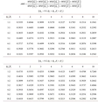
[image:18.595.195.537.368.726.2]

MSE is smaller for MEEL estimators than their counterpart for MM estimators. Furthermore, we also have a chi-square goodness-of-fit statistics for model se-lection for a model without closed form density function. This model testing statistics can be useful for applications in general. Despite the study is limited as

Table 1. Overall relative efficiency of MEEL estimators versus MM estimators.

( )

1 2 12 1 2

ф ф ф

ARE

β β

+ + + +

=

+ + + +

(ф12=0.1,ф1=ф ,2 β1=β2)

1 1

ф β ₁ ₂ ₃ ₄ ₅ ₆ ₈ ₁₀

1.1 0.5335 0.4046 0.3099 0.3170 0.2127 0.1783 0.1514 0.1941 3.1 0.5033 0.4405 0.4408 0.4868 0.4508 0.3161 0.2532 0.2392 4.1 0.3655 0.4629 0.4102 0.3506 0.2924 0.3418 0.2921 0.2859 5.1 0.4405 0.4374 0.3374 0.3913 0.3246 0.3063 0.3119 0.2887 6.1 0.3717 0.3741 0.4499 0.3476 0.3316 0.3269 0.2876 0.3398 8.1 0.3920 0.3778 0.3682 0.3296 0.2768 0.3011 0.2322 0.2613 10.1 0.3221 0.3597 0.2950 0.3032 0.3414 0.2836 0.2186 0.2562

(ф12=0.2,ф ф ,1= 2 β1=β2)

1 1

ф β ₁ ₂ ₃ ₄ ₅ ₆ ₈ ₁₀

(19)

we do not have large computing resources but it does confirm the asymptotic results on efficiencies of MEEL estimators. More works need to be done for as-sessing the efficiencies of MEEL methods by using various parametric models especially in finite samples.

6. Conclusion

MEEL estimators using the proposed moment conditions or bases appear to have the potential of higher efficiencies than MM estimators in general. The methods also provide chi-square goodness-of-fit test statistics for model testing. These features make the methods useful for inferences for bivariate distributions with closed form BLTs or BMGFs without closed form for the bivariate density func-tions. For these distributions, the implementation of likelihood methods might be difficult.

Acknowledgements

The helpful and constructive comments of a referee which lead to an improvement of the presentation of the paper and support form the editorial staffs of Open Journal of Statistics to process the paper are all gratefully acknowledged.

References

[1] Ruijter, M.J. and Oosterlee, C.W. (2012) Two Dimensional Fourier Cosine Series Expansion Method for Pricing Financial Options. SIAM Journal of Scientific Com-puting, 34, B642-B671.https://doi.org/10.1137/120862053

[2] Partrat, C. (1995) Compound Model for Two Dependent Kinds of Claims. Insur-ance: Mathematics and Economics, 15, 219-231.

https://doi.org/10.1016/0167-6687(94)90796-X

[3] Crowder, M. (2012) Multivariate Survival Analysis and Competing Risks. CRC Press, Boca Raton.https://doi.org/10.1201/b11893

[4] Abate, J. and Whitt, W. (1996) An Operational Calculus for Probability Distribu-tions. Advanced in Applied Probability, 28, 75-113.

https://doi.org/10.2307/1427914

[5] Shih, J.H. and Louis, T.A. (1995) Inferences of the Association Parameter in Copula Models for Bivariate Survival Data. Biometrics, 51, 1384-1399.

https://doi.org/10.2307/2533269

[6] Marshall, A.W. and Olkin, I. (1988) Families of Multivariate Distributions. Journal of the American Statistical Association, 83, 834-841.

https://doi.org/10.1080/01621459.1988.10478671

[7] Luong, A. (2017) Maximum Entropy Empirical Likelihood Methods Based on Laplace Transforms for Nonnegative Continuous Distribution with Actuarial Ap-plications. Open Journal of Statistics, 7, 459-482.

https://doi.org/10.4236/ojs.2017.73033

[8] Marshall, A.W. and Olkin, I. (1967) A Multivariate Exponential Distribution. Jour-nal of the American Statistical Association, 62, 30-44.

https://doi.org/10.1080/01621459.1967.10482885