Rational approximations to rational models : alternative algorithms for category learning

warwick.ac.uk/lib-publications

Sanborn, Adam N., Griffiths, Thomas L. and Navarro, Daniel J. (2010) Rational approximations to rational models : alternative algorithms for category learning. Psychological Review, Vol.117 (No.4). pp. 1144-67.

Permanent WRAP URL:

http://wrap.warwick.ac.uk/36000

Copyright and reuse:

The Warwick Research Archive Portal (WRAP) makes this work by researchers of the University of Warwick available open access under the following conditions. Copyright © and all moral rights to the version of the paper presented here belong to the individual author(s) and/or other copyright owners. To the extent reasonable and practicable the material made available in WRAP has been checked for eligibility before being made available.

Copies of full items can be used for personal research or study, educational, or not-for-profit purposes without prior permission or charge. Provided that the authors, title and full

bibliographic details are credited, a hyperlink and/or URL is given for the original metadata page and the content is not changed in any way.

Publisher’s statement: © APA 2010

http://dx.doi.org/10.1037/a0020511

"This article may not exactly replicate the authoritative document published in the APA journal. It is not the copy of record."

A note on versions:

The version presented here may differ from the published version or, version of record, if you wish to cite this item you are advised to consult the publisher’s version. Please see the ‘permanent WRAP URL’ above for details on accessing the published version and note that access may require a subscription.

Running head: RATIONAL APPROXIMATIONS TO CATEGORY LEARNING

Rational approximations to rational models:

Alternative algorithms for category learning

Adam N. Sanborn

Gatsby Computational Neuroscience Unit, University College London

Thomas L. Griffiths

University of California, Berkeley

Daniel J. Navarro

University of Adelaide

Send Correspondence To:

Adam Sanborn

Gatsby Computational Neuroscience Unit

17 Queen Square

London WC1N 3AR

United Kingdom

+44 07942 551970

Abstract

Rational models of cognition typically consider the abstract computational problems

posed by the environment, assuming that people are capable of optimally solving those

problems. This differs from more traditional formal models of cognition, which focus on

the psychological processes responsible for behavior. A basic challenge for rational models

is thus explaining how optimal solutions can be approximated by psychological processes.

We outline a general strategy for answering this question, namely to explore the

psychological plausibility of approximation algorithms developed in computer science and

statistics. In particular, we argue that Monte Carlo methods provide a source of “rational

process models” that connect optimal solutions to psychological processes. We support

this argument through a detailed example, applying this approach to Anderson’s (1990,

1991) Rational Model of Categorization (RMC), which involves a particularly challenging

computational problem. Drawing on a connection between the RMC and ideas from

nonparametric Bayesian statistics, we propose two alternative algorithms for approximate

inference in this model. The algorithms we consider include Gibbs sampling, a procedure

appropriate when all stimuli are presented simultaneously, and particle filters, which

sequentially approximate the posterior distribution with a small number of samples that

are updated as new data become available. Applying these algorithms to several existing

datasets shows that a particle filter with a single particle provides a good description of

Rational approximations to rational models:

Alternative algorithms for category learning

Rational models of cognition aim to explain human thought and behavior as an

optimal solution to the computational problems that are posed by our environment

(Anderson, 1990; Chater & Oaksford, 1999; Marr, 1982; Oaksford & Chater, 1998). This

approach has been used to model several aspects of cognition, including memory

(Anderson, 1990; Shiffrin & Steyvers, 1997), reasoning (Oaksford & Chater, 1994),

generalization (Shepard, 1987; Tenenbaum & Griffiths, 2001a), and causal induction

(Anderson, 1990; Griffiths & Tenenbaum, 2005). However, executing optimal solutions to

these problems can be extemely computationally expensive, a point that is commonly

raised as an argument against the validity of rational models (e.g., Gigerenzer & Todd,

1999; Tversky & Kahneman, 1974). This establishes a basic challenge for advocates of

rational models of cognition: identifying psychologically plausible mechanisms that would

allow the human mind to approximate optimal performance.

The question of how rational models of cognition can be approximated by

psychologically plausible mechanisms addresses a fundamental issue in cognitive science:

bridging levels of analysis. Rational models provide answers to questions posed at Marr’s

(1982) computational level – questions about the abstract computational problems

involved in cognition. This is a different kind of explanation to those provided by other

modeling approaches, which tend to operate at the level of algorithms, considering the

concrete processes that are assumed to operate in the human mind. Theories developed at

these different levels of analysis provide different kinds of explanations for human

behavior, with the computational level explainingwhy we do the things we do, and the

algorithmic level explaininghow these things are done. Both levels of analysis contribute

of bird flight is informed by knowing both how the shape of wings results from

aerodynamics and how those wings are articulated by muscle and bone.

Despite the importance of both the computational and algorithmic level to

understanding human cognition, there has been relatively little consideration of how the

two levels might be connected. In differentiating these levels of analysis, Marr (1982)

clearly stated that they were not independent, with the expectation that results yielded at

one level would provide constraints on theories at another. However, accounts of human

cognition are typically offered at just one of these levels, offering theories of either the

abstract computational problem or the psychological processes involved. Cases where

rational and process models can be explicitly connected are rare and noteworthy, such as

the equivalence of exemplar and prototype models of categorization to different forms of

density estimation (Ashby & Alfonso-Reese, 1995), although recent work has begun to

explore how rational models might be converted into process models (e.g., Kruschke,

2006b).

Considering the processes by which human minds might approximate optimal

solutions to computational problems thus provides us with an opportunity not just to

address a challenge for rational models of cognition, but to consider how one might

develop a general strategy for bridging levels of analysis. In this paper, we outline a

strategy that is applicable to rational analyses of probabilistic inference tasks. In such

tasks, the learner needs to repeatedly update a probability distribution over hypotheses as

more information about those hypotheses becomes available. Due to the prevalence of

such tasks, our strategy provides tools that can be used to derive rational approximations

to a variety of rational models of cognition.

The key idea behind our approach is that efficient implementation of probabilistic

inference is not just a problem in cognitive science – it is an issue that arises in computer

introduction and examples, see Bishop, 2006; Hastie, Tibshirani, & Friedman, 2001;

Mackay, 2003). These algorithms often provide asymptotic guarantees on the quality of

the approximation they provide, meaning that with sufficient resources they can

approximate the optimal inference to any desired level of precision. The existence of these

algorithms suggests a strategy for bridging levels of analysis: starting with rational

models, and then considering efficient approximations to those models as candidates for

psychological process models. The models inspired by these algorithms will not be

rational models, but instead will be process models that are closely tied to rational

models, and typically come with guarantees of good performance as approximations – a

kind of “rational process model”.

Our emphasis in this paper will be on one class of approximation algorithms: Monte

Carlo algorithms, which approximate a probability distribution with a set of samples from

that distribution. Sophisticated Monte Carlo schemes provide methods for sampling from

complex probability distributions (Gilks, Richardson, & Spiegelhalter, 1996), and for

recursively updating a set of samples from a distribution as more data are obtained

(Doucet, Freitas, & Gordon, 2001). These algorithms provide an answer to the question of

how learners with finite memory resources might be able to maintain a distribution over a

large hypothesis space. We introduce these algorithms in the general case, and then

provide a detailed illustration of how these algorithms can be applied to one of the first

rational models of cognition: Anderson’s (1990, 1991) rational model of categorization.

Our analysis of Anderson’s rational model of categorization draws on a surprising

connection between this model and work on density estimation in nonparametric Bayesian

statistics. This connection allows us to identify two new algorithms that can be used in

evaluating the predictions of the model. These two algorithms both asymptotically

approximate ideal Bayesian inference, and help to separate the predictions that arise from

evaluate these algorithms by comparing the results to the full posterior distribution and to

human data. The new algorithms better approximate the posterior distribution and fit

human data at least as well as the original algorithm proposed by Anderson. In addition,

we show that these new algorithms have greater psychological plausibility and provide

better fits to data that have proved challenging to Bayesian models. These results

illustrate the use of rational process models to explain how people perform probabilistic

inference, provide a tool for exploring the relationship between rational models and

human performance, and begin to bridge the gap between computational and algorithmic

levels of analysis.

The plan of the paper is as follows. In the first part of the paper we describe the

general approach. We begin with a discussion of the challenges associated with performing

probabilistic inference, followed by a description of various Monte Carlo methods that can

be used to address these challenges, leading finally to the development of the rational

approximation framework. In the second part of the paper, we apply the rational

approximation idea to categorization problems, using Anderson’s rational model. We first

describe this model, and use its connection to nonparametric statistics to motivate new

approximate inference algorithms. We then evaluate the psychological plausibility of these

algorithms at both a descriptive level and with comparisons to human performance in

several categorization experiments.

The challenges of probabilistic inference

The computational problems that people need to solve are often inductive problems,

requiring an inference from limited data to underdetermined hypotheses. For example,

when learning about a new category of objects, people need to infer the structure of the

category from examples of its members. This inference is inherently inductive, since the

learner; and because of this, it is not possible to know exactly which structure is correct.

That is, the optimal solution to problems of this kind requires the learner to make

probabilistic inferences, evaluating the plausibility of different hypotheses in light of the

information provided by the observed data. In the remainder of this section, we discuss

two challenges that a learner attempting to implement the ideal solution faces: reasoning

about hypotheses that are composed of large numbers of variables, and repeatedly

updating beliefs about a set of hypotheses as more information becomes available over

time.

Reasoning about large numbers of variables

One of the most fundamental challenges in performing probabilistic inference

concerns the situation when the number of hypotheses is very large. This is typically

encountered when each hypothesis corresponds to a statement about a number of different

variables. The number of hypotheses then suffers from a combinatoric explosion. For

example, many theories of category learning assume that people assign objects to clusters.

If so, then each hypothesis is composed of many assignment variables, one per object.

Likewise, in causal learning, hypotheses about causal structure can often be expressed in

terms of all of the individual causal relationships that make up a given structure, thus

requiring multiple variables. Reasoning about hypotheses comprised of large numbers of

variables poses a particular challenge, because of the combinatorial nature of the

hypothesis space: the number of hypotheses to be considered can increase exponentially in

the number of relevant variables. The number of possible clusterings of nobjects, for

example, is given by thenth Bell number, with the first ten values being 1, 2, 5, 15, 52,

203, 877, 4140, 21147, and 115975. In such cases, brute force enumeration of all

hypotheses will be extremely computationally expensive, and scale badly with the number

Updating beliefs over time

When making probabilistic inferences, we rarely have all the information we need to

definitively evaluate a hypothesis. As a result, when a learner observes a piece of data and

uses this to form beliefs, he or she generally remains somewhat uncertain about which

hypothesis is really the correct one. When a new piece of information arrives, this

distribution needs to be updated to the new beliefs. The consequence is that an ideal

learner needs to constantly update a probability distribution over hypotheses as more data

are observed.

Updating beliefs over time is computationally challenging because it requires the

learner to draw inferences every time new information becomes available. Unless the

learner uses methods that allow the efficient updating of his or her beliefs, he or she would

be required to perform the entire inference from scratch every time new information

arrives. The cost of probabilistic inference is thus multiplied by the number of

observations that have to be processed. As one would expect, this becomes particularly

expensive with large hypothesis spaces, such as the combinatorial spaces that result from

having hypotheses expressed over large numbers of random variables. Making

probabilistic inference computationally tractable thus requires developing strategies for

efficiently updating a probability distribution over hypotheses as new data are observed.

Algorithms to address the challenges

Some of the challenges of probabilistic inference can be addressed by approximating

optimal solutions using algorithms based on the Monte Carlo principle. This principle is

one of the most basic ideas in statistical computing: rather than performing computations

using a probability distribution, we perform those computations using a set of samples

from that distribution. The resulting approximation becomes increasingly accurate as the

approximation can be used to determine how many samples should be generated. This

principle forms the foundation of an entire class of approximation algorithms (Motwani &

Raghavan, 1996). Monte Carlo methods provide a way to efficiently approximate

probabilistic inference. However, generating samples from posterior distributions is

typically not straightforward: generating samples from a distribution requires knowing the

form that distribution takes, which is a large part of the challenge of probabilistic

inference in the first place. Consequently, sophisticated algorithms need to be used in

order to generate samples. Here we introduce two such algorithms at an intuitive level:

Gibbs sampling and particle filters. A parallel mathematical development of the general

algorithms is given in the Appendix and toy examples of these algorithms applied to

categorization and a discussion of their psychological plausibility are given later.

Gibbs sampling

Gibbs sampling (Geman & Geman, 1984) is a very commonly used Monte Carlo

method for sampling from probability distributions. This algorithm is initialized with a

particular set of values for each variable, often with random values. Gibbs sampling works

on the principle of sampling a single random variable at each step. One random variable is

selected, and the value of this variable is sampled, conditioned on the values of all of the

other random variables and the data. The process is repeated for each variable; each is

sampled conditioned on the values of all of the other variables and the data. Intuitively,

Gibbs sampling corresponds to the process of inspecting one’s beliefs about each random

variable conditioned on one’s beliefs about all of the other random variables, and the data.

Reflecting on each variable in turn provides the opportunity for changes to propagate

through the set of random variables. A complete run through sampling all of the random

variables is an iteration and the algorithm is usually engaged for many iterations.

at a particular, often random, set of values. The early iterations show the algorithm

converging to the desired distribution, but are not yet samples from this distribution.

These iterations are known as theburn-inand are thrown away. An additional difficulty is

that iterations following the burn-in iterations often show strong dependency from one

iteration to the next. These iterations are then thinned, which means keeping everynth

iteration and discarding the rest. The remaining iterations after burn-in and thinning are

used as samples from the desired distribution. This process provides a way to generate

samples from probability distributions defined over large numbers of variables without

ever having to enumerate the entire hypothesis space, providing a tractable way to

perform probabilistic inference in these cases.

Particle filters

A second class of Monte Carlo algorithms, particle filters, are specifically designed to

deal with sequential data. Particle filters are underpinned by a simpler algorithm known

as importance sampling, which is used in cases in which it is hard to sample from the

target distribution, but easy to sample from a related distribution (known as theproposal

distribution). The basic idea of importance sampling is that we generate samples from the

proposal distribution, and then assign those samples weights that correct for the difference

from the target distribution. Samples that are more likely under the proposal than the

target distribution are assigned lower weights, since they should be over-represented in a

set of draws from the proposal distribution, and samples that are more likely under the

target than the proposal are assigned higher weights, increasing their influence.

Particle filters extend importance sampling to a sequence of probability

distributions, typically making use of the relationship between successive distributions to

use samples from one distribution to generate samples from the next (for more details, see

about variables in a dynamic environment – the problem of “filtering” is to infer the

current state of the world given a sequence of observations. However, it also provides a

natural solution to the general problem of updating a probability distribution over time.

Each particle is a sample from the posterior distribution on the previous trial, and these

samples are updated when new data become available.

Rational approximations to rational models

Monte Carlo algorithms provide efficient schemes for approximating probabilistic

inference, and come with the asymptotic guarantee that they can produce an arbitrarily

good approximation if sufficient computational resources are available. These algorithms

thus seem like good candidates for explaining how human minds could be capable of

performing probabilistic inference, bridging the gap between the computational-level

analyses typically associated with rational models of cognition and the algorithmic level at

which psychological process models are defined. In particular, Gibbs sampling and particle

filters provide solutions to the challenges posed by probabilistic inference with large

numbers of variables and updating probability distributions over time.

Part of the attraction of the Monte Carlo principle as the basis for developing

rational process models is that it reduces probabilistic computations to one operation:

generating samples from a probability distribution. The notion that people might be

capable of generating samples from internalized probability distributions has previously

appeared in psychological process models of decision making (Stewart, Chater, & Brown,

2006), estimation (Fiedler & Juslin, 2006), and prediction (Mozer, Pashler, & Homaei,

2008). Indeed, the foundational premise of the highly successful “sequential sampling”

framework (Ratcliff, 1978; P. L. Smith & Ratcliff, 2004; Vickers, 1979) is that choice

behavior is fundamentally reliant on people drawing and evaluating samples from

representations (Lee & Cummins, 2004; Ratcliff, 1978; Vandekerckhove, Verheyen, &

Tuerlinckx, 2010). Taken together, these models provide support for the idea that the

basic ingredients required for Monte Carlo simulation are already part of the psychological

toolbox.

Recent research has also identified correspondences between the kind of

sophisticated Monte Carlo methods discussed above and psychological process models.

Shi, Feldman, and Griffiths (2008) showed that the basic computations involved in

importance sampling are identical to those used in exemplar models (also see Shi, Griffiths,

Feldman, & Sanborn, in press). Exemplar models assume that people store stimuli in

memory, activating them based on their similarity to new stimuli (e.g., Medin & Schaffer,

1978; Nosofsky, 1986). An importance sampler can be implemented by storing hypotheses

in memory, and activating them in proportion to the probability of observed data under

that hypothesis. Moreover, this interpretation of exemplars as stored hypotheses links

exemplar-based learning nicely to previous rational analyses of exemplar-based decisions

as a form of sequential analysis (see Navarro, 2007; Nosofsky & Palmeri, 1997). That is,

the importance sampling method allows people to efficiently learn and store a posterior

distribution, and the sequential analysis method allows efficient decisions to be made on

the basis of this stored representation. This thus constitutes a natural, psychologically

plausible scheme for approximating some probabilistic computations.

Several recent papers have also examined the possibility that particle filters might

be relevant to understanding how people can update probability distributions over time.

This idea was first raised by Sanborn, Griffiths, and Navarro (2006), and particle filters

have subsequently been used to explain behavioral patterns observed in several tasks.

Daw and Courville (2008) argued that a particle filter with a small number of particles

could explain rapid transitions seen in associative learning tasks with animals. Brown and

detection task, where variation of the number of particles being considered captured one

dimension along which participants varied. Finally, Levy, Reali, and Griffiths (2009)

showed that garden path effects in sentence processing could be accounted for by using a

particle filter for parsing, where the frequency with which the parser produced no valid

particles was predictive of the difficulty that people had interpreting the sentence.

Evaluating Monte Carlo algorithms as candidates for rational process models

requires exploring how the predictions of rational models of cognition vary under these

different approximation schemes, and examining how well these predictions correspond to

human behavior. In the remainder of the paper, we provide a detailed investigation of the

performance of different approximation algorithms for Anderson’s (1990; 1991) rational

model of categorization. This model is a good candidate for such an investigation, since it

involves an extremely challenging computational problem: evaluating a posterior

distribution over all possible partitions of a set of objects into clusters. This problem is so

challenging that Anderson’s original presentation of the model resorted to a heuristic

solution. We use a connection between this rational model and a model that is widely

used in Bayesian statistics to specify a Gibbs sampler and particle filter for this model,

which we evaluate against a range of empirical data.

The Rational Model of Categorization

The problem of category learning is to infer the structure of categories from a set of

stimuli labeled as belonging to those categories. The knowledge acquired through this

process can ultimately be used to make decisions about how to categorize new stimuli.

Several rational analyses of category learning have been proposed (Anderson, 1990; Ashby

& Alfonso-Reese, 1995; Nosofsky, 1998). These analyses essentially agree on the nature of

the computational problem involved, casting category learning as a problem ofdensity

labels. Viewing category learning in this way helps to clarify the assumptions behind the

two main classes of psychological models: exemplar models and prototype models.

Exemplar models assume that a category is represented by a set of stored exemplars, and

categorizing new stimuli involves comparing these stimuli to the set of exemplars in each

category (e.g., Medin & Schaffer, 1978; Nosofsky, 1986). Prototype models assume that a

category is associated with a single prototype and categorization involves comparing new

stimuli to these prototypes (e.g., Reed, 1972). These approaches to category learning

correspond to different strategies for density estimation used in statistics, being

nonparametric and parametric density estimation respectively (Ashby & Alfonso-Reese,

1995).

Anderson’s (1990, 1991) rational analysis of categorization takes a third approach,

modeling category learning as Bayesian density estimation. This approach encompasses

both prototype and exemplar representations, automatically selecting the number of

clusters to be used in representing a set of objects. Unfortunately, the inference for this

model is extremely complex, requiring an evaluation of every possible way of partitioning

exemplars into clusters, with the number of possible partitions growing exponentially with

the number of exemplars. Anderson proposed an approximation algorithm in which stimuli

are sequentially assigned to clusters, and assignments of stimuli are fixed once they are

made. However, this algorithm does not provide any asymptotic guarantees for the quality

of the resulting assignments, and is extremely sensitive to the order in which stimuli are

observed, a property which is not intrinsic to the underlying statistical model. As a result,

evaluations of the model are tied to the particular approximation algorithm that was used.

Before we consider alternative approximation algorithms for Anderson’s model, we

need to provide a detailed specification of the model and the original algorithm. In this

section, we first outline the Bayesian view of categorization, showing how exemplar and

approach taken by Anderson.

Bayesian categorization models

Rational models of categorization must solve the density estimation problem

outlined above and use this estimate to identify the category label or some other

unobserved property of an object using its observed properties (Anderson, 1990; Ashby &

Alfonso-Reese, 1995; Rosseel, 2002). This prediction problem has a natural interpretation

as a form of Bayesian inference, which we now outline. Suppose that the learner has

previously been shown a set of two stimuli and their labels, where the two stimuli are the

first two stimuli in Figure 1. We letyi refer to the category label given to theith object in

this list (often a nonsense syllable such as “DAX”), and the mental representation of the

object is assumed to be characterized by a collection of features, denotedxi. So for

instance if the stimulus is the first stimulus, it could be simply described in terms of

features such as “is circular”, “is black”, and “is large”. Thus, if the learner is told “the

first stimulus is a DAX”, we would describe the trial by the pair (xi, yi). Across the set of

two labelled objects, the information available to the learner can be thought of as a

collection of statements (e.g., “the first stimulus is a DAX” and “the second stimulus is a

ZUG”) that can be formally characterized by the collection of stimulus representations

x2 = (x1, x2), along with the labels given to each of these objectsy2= (y1, y2). More

generally we will refer to these already known stimuli as the firstN −1 stimuli with

representationsxN−1= (x1, x2, . . . xN−1), and labelsyN−1 = (y1, y2, . . . yN−1)

With that in mind, the problem facing the learner can be written in the following

way: on the Nth trial in the experiment, he or she is shown a new stimulusxN (e.g., the

third stimulus in Figure 1), and asked what label it should be given. If there are J

possible labels involved in the task, the problem is to determine if the Nth object should

(xN,xN−₁,yN−₁). If we apply Bayes’ rule to this problem, we are able to see that

P(yN =j|xN,xN−1,yN−1) = P(xN|yN =j,

xN−1,yN−1)P(yN =j|yN−1)

!J

y=1P(xN|yN =y,xN−₁,yN−₁)P(yN =y|yN−₁)

. (1)

In this expression,P(xN|yN =j,xN−1,yN−1) denotes the estimated probability that an

element of thejth category would possess the collection of featuresxN observed in the

novel object, andP(yN =j|yN−₁) is an estimate of the prior probability that a new

object would belong to thejth category. Additionally, we have assumed that the prior

probability of an object coming from a particular category is independent of the features

of the previous objects. Thus, this expression makes clear that the probability that an

object with featuresxN should be given the labelyN =j is related both the probability of

sampling an object with featuresxN from that category, and the prior probability of

choosing that category label. Category learning, then, becomes a matter of determining

these probabilities – the problem known as density estimation.

One advantage to describing categorization in terms of the density estimation

problem is that both exemplar models and prototype models can be described as different

methods for determining the probabilities described by Equation 1. Specifically, Ashby

and Alfonso-Reese (1995) observed that if the learner uses a simple form of nonparametric

density estimation known as kernel density estimation (e.g., Silverman, 1986) in order to

compute the probabilityP(xN|yN =j,xN−1,yN−1), then an exemplar model of

categorization is the result. On the other hand, they note that the learner could use a

form of parametric density estimation (e.g., Rice, 1995), in which the category

distribution is assumed to have some known form, and the learner’s goal is to estimate the

unknown parameters of that distribution. If the learner uses this approach, then the result

is a prototype model, with the centroid being an appropriate estimate for distributions

whose parameters characterize their mean. To illustrate the point, Figure 2 shows a

distribution centered over the prototype, and an exemplar model on the right, in which a

separate normal distribution (the “kernel”) is placed over each exemplar, and the resulting

category distribution is a mixture model.

Having cast the problem in these terms, it is clear that exemplar and prototype

models are two extremes along a continuum of possible approaches to category

representation. As illustrated in the middle panel of Figure 2, the learner might choose to

break the category up into several clusters of stimuli, denotedzN−1, wherezi=kif the

ith stimulus is assigned to thekth cluster. Each such cluster is then associated with a

simple parametric distribution, and the category distribution as a whole then becomes a

mixture model (e.g. Rosseel, 2002; Vanpaemel & Storms, 2008). Expressed in these terms,

prototype models map naturally onto the idea of a one-cluster representation, and

exemplar models arise when there is a separate cluster for each object. In between lies a

whole class of intermediate category representations, such as the one shown in the middle

of Figure 2. In this case, the learner has divided the five objects into two clusters, and the

resulting category distribution is a mixture of two normal distributions.

The appeal of this more general class of category representations is that it allows

people to use prototype-like models when called for, and to move to the more flexible

exemplar-like models when needed. However, by proposing category representations of

this form, we introduce a new problem: for a set ofN objects how many clustersK are

appropriate to represent the categories, and how should the cluster assignmentszN be

made in light of the available data (xN,yN)? It is to this topic that we now turn.

Statistical model

A partial solution to this problem was given by Anderson (1990), in the form of the

Rational Model of Categorization (RMC). The RMC is somewhat different to the various

being equivalent to unobserved features. As a consequence, the RMC specifies a joint

distribution on features and category labels, rather than assuming that the distribution

over category labels is estimated separately and then combined with a distribution on

features for each category. This distribution is a mixture, with

P(xN,yN) = "

zN

P(xN,yN|zN)P(zN) (2)

whereP(zN) is a distribution over possible partitions of theN objects into clusters.

Importantly, the number of clustersK in the partition zN is not assumed to be fixed in

advance, but is rather something that the learner infers from the data. The RMC provides

an explicit form for this prior distribution, namely

P(zN) =

(1−c)K_cN−K

#N−1

i=0 [(1−c) +ci]

K $

k=1

(Mk−1)! (3)

wherec is a parameter called thecoupling probability, Mk is the number of objects

assigned to cluster k, andK is the total number of clusters inzN. Although this

distribution appears unwieldy, it is in fact the distribution that results from sequentially

assigning objects to clusters with probability

P(zi =k|zi−1) =

       cMk

(1−c)+c(i−₁₎ ifMk>0 (i.e., k is old) (1−c)

(1−c)+c(i−₁₎ ifMk= 0 (i.e.,k is new)

(4)

where the counts Mk are accumulated overzi−1. Thus, each object can be assigned to an

existing cluster with probability proportional to the number of objects already assigned to

that cluster, or to a new cluster with probability determined byc. Since the prior

distribution is set up in a way that allowsK to grow as more objects are encountered, the

RMC allows the learner to infer the number of clusters via the usual process of Bayesian

updating.

Intuitively, we can look at the prior as a rich-get-richer scheme: if a cluster already

coupling probability is the parameter that determines the severity of this scheme. For

high values of the coupling parameter, then larger clusters will be favored in the prior,

while for low values of the coupling parameter, smaller clusters will be favored. The

cluster sizes that actually result depend on the likelihoods as well as the prior.

The local MAP algorithm

When considering richer representations than prototypes and exemplars it is

necessary to have a method for learning the appropriate representation from data. Using

Equation 2 to make predictions about category labels and features requires summing over

all possible partitionszN. This sum rapidly becomes intractable for large N, since the

number of partitions grows rapidly with the number of stimuli according to the Bell

number introduced earlier. Consequently, an approximate inference algorithm is needed

and Anderson (1990, 1991) developed a simple inference algorithm to solve this problem.

We will refer to this algorithm as thelocal MAPalgorithm, as it involves assigning each

stimulus to the cluster that has the highest posterior probability given the previous

assignments (i.e., the maximum a posteriori or MAP cluster). The algorithm is a local

implementation of the MAP because it makes an assignment for each new stimulus as it

arrives, which does not necessarily result in the global MAP.

The local MAP algorithm approximates the sum in Equation 2 with just a single

clustering of theN objects,zN. This clustering is selected by assigning each object to a

cluster as it is observed. At this point, the features and labels of all stimuli, along with

the cluster assignments zi−₁ for the previousi−1 stimuli are given. Thus, the posterior

probability that stimulusiwas generated from cluster k is

P(zi =k|zi−₁, xi,xi−₁, yi,yi−₁)∝ (5)

P(xi|zi =k,zi−1,xi−1)P(yi|zi =k,zi−1,yi−1)P(zi =k|zi−1)

assigned to the cluster kthat maximizes Equation 5. Iterating this process results in a

single partition of a set ofN objects.

To illustrate the local MAP algorithm, we show in Figure 3 how it would be applied

it to the simple example of sequentially presented stimuli in Figure 1. Each stimulus is

parameterized by three binary features and the likelihood

P(xi|zi=k,zi−1,xi−1)P(yi|zi=k,zi−1,yi−1) is calculated using binomial distributions

that are independent for each feature. These binomial likelihoods are parameterized by

the probability of the outcome, and need a prior distribution over this probability. The

standard prior for binomial likelihoods is the Beta distribution (see the Appendix for

details). For the toy example, we used a symmetric Beta prior for the binomial likelihood,

withβ = 1. The symmetric Beta distribution withβ= 1 is a simple choice, because it is

equivalent to the uniform distribution.

The local MAP algorithm initially assigns the first observed stimulus to its own

cluster. When the second stimulus is observed, the algorithm generates each possible

partition: either it is assigned to the same cluster as the first stimulus or to a new cluster.

The posterior probability of each of these partitions is calculated and the partition with

the highest posterior probability is always chosen as the representation. After the third

stimulus is observed, the algorithm produces all possible partitions involving the third

stimulus, assuming that the clustering for the first two stimuli remains the same. Note

that not all possible partitions of the three stimuli are considered, because the algorithm

makes an irrevocable choice for the partition of the first two stimuli and the possible

partitions on later trials have to be consistent with this choice. The local MAP algorithm

will always produce the same final partition for a given sequential order of the stimuli,

assuming there are no ties in the posterior probability.

this partition. In effect, it assumes that

P(xN,yN)≈P(xN,yN|zN) (6)

wherezN is produced via the procedure outlined above. The probability that a particular

object receives a particular category label would likewise be computed using a single

partition.

Summary

The RMC specifies a rational model of categorization, capturing many of the ideas

embodied in other models and allowing the representation to be inferred from the data.

However, the model is still significantly limited, because the approximate algorithm used

for assigning objects to clusters in the RMC can be a poor approximation to the posterior.

In particular, this makes it hard to discriminate the predictions that result from the

underlying statistical model from those that are a consequence of the algorithm being

used. In order to explore alternative approximation algorithms, we now discuss the

connections between the RMC and nonparametric Bayesian statistics.

Dirichlet process mixture models

One of the most interesting properties of the RMC is that it has a direct connection

to a model used in nonparametric Bayesian statistics (Neal, 1998). The rationale for using

nonparametric methods is that real data are not generally sampled from some neat,

finite-dimensional family of distributions, so it is best to avoid this assumption at the

outset. From a Bayesian perspective, the nonparametric approach requires us to use priors

that include as broad a range of densities of possible, thereby allowing us to infer very

complex densities if they are warranted by data. The most commonly used method for

placing broad priors over probability distributions is theDirichlet process (DP; Ferguson,

infinite mixtures of point masses (Sethuraman, 1994), making them ideally suited to act

as priors in infinite mixture models (Escobar & West, 1995; Rasmussen, 2000). When used

in this fashion, the resulting model is referred to as aDirichlet process mixture model

(DPMM; Antoniak, 1974; Ferguson, 1983; Neal, 1998).

Although a complete description of the Dirichlet process is beyond the scope of this

paper (for more details, see Navarro, Griffiths, Steyvers, & Lee, 2006), what matters for

our purposes is that the Dirichlet process implies a distribution over partitions: any two

observations in the sample that were generated from the same mixture component may be

treated as members of the same cluster, allowing us to specify priors over an unbounded

number of clusters. In the case whereN observations have been made, the prior

probability that a Dirichlet process will partition those observations into the clusterszN is

P(zN) =

αK

#N−1

i=0 [α+i]

K $

k=1

(Mk−1)! (7)

whereα is the dispersion parameter of the Dirichlet process. This distribution over

partitions can be produced by a simple sequential stochastic process (Blackwell &

MacQueen, 1973). If observations are assigned to clusters one after another and the

probability that observationi+ 1 is assigned to clusterk is

P(zi =k|zi−₁) =

       Mk

i−1+α ifMk >0 (i.e., kis old)

α

i−1+α ifMk= 0 (i.e., kis new)

(8)

we obtain Equation 7 for the probability of the resulting partition. This distribution has a

number of nice properties, with one of the most important beingexchangeability: the prior

probability of a partition is unaffected by the order in which the observations are received

(Aldous, 1985). Intuitively, exchangeability is similar to independence, but slightly weaker.

To make some of these ideas more concrete, Figure 4 presents a visual depiction of

the relationship between the partitioning implied by the DP, the distribution over

stimuli that results in the DPMM. The partitioning implied by the DPMM shows that

items are divided into discrete clusters. Each of these clusters is given a parameter drawn

from the prior distribution over parameters. A large number of parameter draws are

shown in Figure 4b. Each spike is a new parameter value and the height of the bars

depends on the number of clusters that use that parameter. Finally, combining the

parameter values with a continuous likelihood function, such as a Gaussian distribution,

gives the mixture distribution shown in Figure 4c.

It should be apparent from our description of the prior distribution used in the

DPMM that it is similar in spirit to the prior distribution underlying the RMC. In fact,

the two are directly equivalent, a point that was first made in the statistics literature by

Neal (1998). If we letα= (1−c)/c, Equations 3 and 7 are equivalent, as are Equations 4

and 8. Thus the prior over cluster assignments used in the RMC is exactly the same as

that used in the DPMM. Anderson (1990, 1991) thus independently discovered one of the

most celebrated models in nonparametric Bayesian statistics, deriving this distribution

from first principles.

Alternative approximate inference algorithms

The connection between the RMC and the DPMM suggests a solution to the

shortcomings of the local MAP algorithm. In this section, we draw on the extensive

literature on approximate inference for DPMMs to offer two alternative algorithms for the

RMC: Gibbs sampling and particle filtering. These algorithms are less sensitive to order

and are asymptotically guaranteed to produce accurate predictions.

As discussed above, both Gibbs sampling and particle filters are Monte Carlo

methods. This means that they provide ways of approximating the intractable sum over

partitions numerically using a collection of samples. Specifically, to compute the

approximation gives

P(yN =j|xN,yN−1) =

"

zN

P(yN =j|xN,yN−1,zN)P(zN|xN,yN−1) (9)

≈ 1

M

M "

"=1

P(yN =j|xN,yN−1,z(N"))

wherez(1)_N , . . . ,z(_NM) areM samples fromP(zN|xN,yN−1), and the approximation becomes

exact asM → ∞. The two algorithms differ only in how these samples are generated.

Gibbs sampling

Gibbs sampling is the approximate inference algorithm most commonly used with

the DPMM (e.g., Escobar & West, 1995; Neal, 1998). It provides a way to construct a

Markov chain that converges to the posterior distribution over partitions. The state space

of the Markov chain is the set of partitions, and transitions between states are produced

by sampling the cluster assignment of each stimulus from its conditional distribution,

given the current assignments of all other stimuli. The clustering evolves by sequentially

sampling each zi from the distribution

P(zi =k|z−i, xi,x−i, yi,y−i)∝ (10)

P(xi|zi =k,z−i,x−i)P(yi|zi=k,z−i,y−i)P(zi =k|z−i)

wherez−i refers to all cluster assignments except for theith.

Equation 10 is extremely similar to Equation 5, although it gives the probability of

a cluster based on the all of the trials in the entire experiment except for the current trial,

instead of just the previous trials. The statistical property of exchangeability, briefly

noted above, means that these probabilities are actually computed in exactly the same

way: the order of the observations can be rearranged so that any particular observation is

considered the last observation. Hence, we can use Equation 8 to computeP(zi|z−i), with

being chosen with probability determined byα (or, equivalently,c). The other terms

reflect the probability of the features and category label of stimulus iunder the partition

that results from this choice ofzi, and depends on the nature of the features.

The Gibbs sampling algorithm for the DPMM is straightforward (Neal, 1998), and

is illustrated for the simple example in Figure 5. First, an initial assignment of stimuli to

clusters is chosen, with a convenient choice being all stimuli assigned to a single cluster.

Unlike the local MAP algorithm, Gibbs sampling is not a sequential algorithm; all stimuli

must be observed before it can be run. Next, we choose a single stimulus and consider all

possible reassignments of that stimulus to clusters, including not making a change in

assignments or assigning the stimulus to a new cluster. Equation 10 gives the probability

of each partition and one of the partitions is sampled based on its posterior probability,

making this algorithm stochastic, unlike the local MAP. The stochastic nature of the

algorithm is evident in the example in Figure 5, because the first circled assignment has

lower probability than the alternatives. The example shows two iterations of Gibbs

sampling, in which each stimulus is cycled through and reassigned. In an actual

application the algorithm would go through many iterations, with the output of one

iteration providing the input to the next. Since the probability of obtaining a particular

partition after each iteration depends only on the partition produced on the previous

iteration, this is a Markov chain.

After enough iterations for the Markov chain to converge, we begin to save the

partitions it produces. The partition produced on one iteration is not independent of the

next, so the results of some iterations are discarded to approximate independence. The

partitions generated by the Gibbs sampler can be used in the same way as samplesz(_N") in

Equation 9. As with standard Monte Carlo approximations, the quality of the

approximation increases as the number of partitions in that collection increases. The

Equation 9, and thus of making accurate predictions about the unobserved features of

stimuli.

Particle filtering

There are several ways to construct a particle filter for the DPMM. The method we

will use is most closely related to the one discussed by Fearnhead (2004). The key idea is

to treat each new observation as a new “time step”, with each particle being a partition

z(_i") of the stimuli from the firstitrials. Unlike the local MAP algorithm, in which the

posterior distribution is approximated with a single partition, the particle filter usesM

partitions. Summing over these particles gives us an approximation to the posterior

distribution over partitions

P(zi|xi,yi)≈ M "

"=1

1

Mδ(zi,z (")

i ) (11)

whereδ(z,z") is 1 whenz=z", and 0 otherwise. If Equation 11 is used as an

approximation to the posterior distribution over partitionszi after the first itrials, then

we can approximate the distribution ofzi+1 given the observationsxi,yi in the following

manner:

P(zi₊₁|xi,yi) = "

zi

P(zi₊₁|zi)P(zi|xi,yi)

≈ "

zi

P(zi+1|zi) m "

!=1

1 mδ(zi,z

(!₎ i ) = 1 m m " !=1

P(zi+1|z(

!₎

i ) (12)

whereP(zi+1|zi) is given by Equation 8. We can then incorporate the information

conveyed by the features and label of stimulusi+ 1, arriving at the approximate posterior

probability

P(zi₊₁|xi₊₁,yi₊₁) ∝ P(xi₊₁|zi₊₁,xi)P(yi₊₁|zi₊₁,yi)P(zi₊₁|xi,yi)

≈ 1 m

m "

!=1

P(xi₊₁|zi₊₁,xi)P(yi₊₁|zi₊₁,yi)P(zi₊₁|z( !₎

The result is a discrete distribution over all the previous particle assignments and all

possible assignments for the current stimulus. DrawingM samples from this distribution

provides us with our new set of particles.

The particle filter for the simple example is illustrated in Figure 6. The particle

filter for the DPMM is initialized with the first stimulus assigned to the first cluster for all

M particles, in this caseM = 2. On observing each new stimulus, the distribution in

Equation 13 is calculated, based on the particles sampled in the last trial. Like the local

MAP, the particle filter updates the partition as each new stimulus is observed, and like

the local MAP, only new partitions that are consistent with the previous choices made by

the algorithm are considered. This consistency can be seen in the potential partitions

when the third stimulus is observed in Figure 6: each descendant is consistent with the

partition choices made by its ancestor. Intuitively, the psychological processes involved in

this approximation are very similar to those involved in the local MAP algorithm. People

update their beliefs incrementally, keeping the assignments of old items fixed, and making

the assignments of new items conditional on these fixed beliefs. There are two key

differences between the local MAP and particle filter algorithms. The first is that the

choice of new partitions is stochastic instead of deterministic. The particle filter algorithm

samples new partitions based on their posterior probabilities instead of always selecting

the partition with the maximum probability. A particle filter withM = 1 particles is

equivalent to the local MAP algorithm, except that the new partition is sampled instead

of deterministically selected. The second difference is that multiple particles means that

multiple partitions can be used instead of the single partition passed forward by the local

MAP. The M partitions are selected without regard for ancestry, allowing a partition that

was selected for the early observations to die out as the descendants of other partitions

Approximation quality

The differences in quality of the various approximations can be explored by a toy

example using sequential observations of the stimuli in Figure 1. We compared the local

MAP, a particle filter withM = 100 particles, a particle filter withM = 1 particle, and

Gibbs sampling to the exact posterior. For each algorithm a symmetric Beta prior in

which β = 1 was used for the likelihood (see Appendix for details). The local MAP was

run a single time, because its outcome is deterministic on a fixed stimulus order. The

particle filters were each replicated 10,000 times, and the Gibbs sampler was run for

101,000 iterations. For the Gibbs sampler, the first 1,000 iterations were discarded and

every 10th iteration was taken as a sample, yielding 10,000 samples. The results of this

comparison are shown in Figure 7. The local MAP algorithm has selected a single

partition as an approximation to the exact posterior. In this example, the partition

selected by the local MAP is also the MAP of the exact posterior distribution, but the two

will not always be equivalent. By taking the MAP partition as each stimulus arrives, the

local MAP can be misled to choose a partition that is not the global MAP, if the initial

trials are not representative of the whole run of trials. An example of this can be seen in

the experiment by Anderson and Matessa in a later section.

The particle filter withM = 100 particles and the Gibbs sampler both produce a

posterior distribution that is nearly indistinguishable from the exact posterior. The

single-particle particle filter is an interesting intermediate case. Each run of the

single-particle particle filter produces a single partition, not the distribution produced by

a particle filter withM >1 particles. However, averaging over runs of the single-particle

particle filter gives an approximation that is much closer to the exact posterior than the

local MAP. Unlike the asymptotic performance of the Gibbs sampler and particle filter

with infinite particles, the approximation of the single-particle particle filter is slightly

algorithm is stochastic, but is still present because each run of the M = 1 particle filter

cannot correct its previous assignments by resampling.

Psychological plausibility of the algorithms

Before turning to a quantitative comparison of the algorithms with human data it is

worth considering their psychological plausibility at a descriptive level, to see whether

they are appropriate for human cognition. We take as a starting point Anderson’s (1990,

1991) two desiderata for an approximate inference algorithm: that it be incremental, and

that people see objects as arising from a single cause. These desiderata were based on

beliefs about the nature of human category learning. In tasks in which people see objects

presented sequentially and must judge which category they arise from “people need to be

able to make predictions all the time not just at particular junctures after seeing many

objects and much deliberation” (Anderson, 1991, p. 412), and “people tend to perceive

objects as coming from specific categories” (Anderson, 1991, p. 411).

In addition to these two desiderata, we are concerned with how these algorithms

might introduce new order effects into a model. Often statistical models, such as the

DPMM, are invariant to the order in which observations arrive. However, the

approximations used in practical applications of these models tend to introduce order

effects as a side effect of limited computation. People show effects of the order of

presentation of stimuli (Anderson, 1990; Medin & Bettger, 1994; Murdock, 1962), and to

have a psychologically plausible algorithm, the cumulative order effects of the model and

those introduced by the approximation should match the order effects displayed by people.

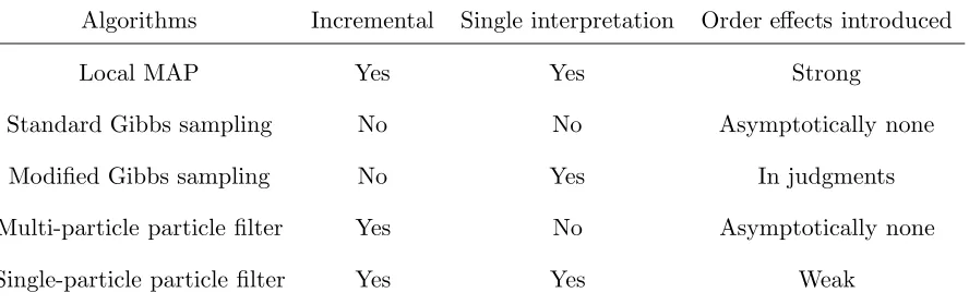
In the remainder of this section we summarize the psychological plausibility of the local

MAP, Gibbs sampling, and particle filters. We relate these algorithms to the properties of

incrementalism, a single interpretation of how the data arise, and the order effects

Local MAP

Anderson (1990, 1991) introduced the local MAP algorithm to satisfy his two

desiderata for psychological plausibility. The first desideratum is satisfied because the

local MAP is updated incrementally. In addition, the second desideratum is satisfied

because only a single partition of the stimuli into clusters is available to the algorithm in

order to make judgments about new stimuli. However, as a result of the single

interpretation and its maximization operation, the local MAP algorithm is extremely

sensitive to the order in which stimuli are observed. For example, Anderson and Matessa

(reported in Anderson, 1990) showed that the predictions of the local MAP algorithm

depended strongly on the order the stimuli were introduced in their clustering experiment.

For one type of order, the local MAP always predicted one partition of the stimuli, but for

the other order it always predicted a second partition. We will explore how the local MAP

can be led down garden paths when we compare the algorithms quantitatively.

Gibbs sampling

Gibbs sampling draws samples from one random variable conditioned on all of the

rest and all of the data, thus requiring all of the data be present before inference begins.

New data cannot be incrementally added to the sampling scheme, so in order to sample

from a posterior distribution when a new piece of data arrives, Gibbs sampling must start

from scratch. This property makes the algorithm computationally wasteful if sequential

judgments are required. For other tasks, however, Gibbs sampling is more psychologically

plausbile. In tasks in which all of the data arrive simultaneously, such as when a

researcher gives participants a set of objects to sort into groups, participants do not need

to make judgments until all of the stimuli are present. Here Gibbs sampling seems

psychologically plausible.

of the data. The algorithm gathers a set of samples from a probability distribution and all

of these samples are used to infer other properties about the data, such as category labels.

However, we should note that it would be possible to implement a modified version of the

Gibbs sampling algorithm that would provide a fixed interpretation of the data. Instead of

keeping all of the iterations, we could create a very forgetful Gibbs sampler that would

only recall the current values of the variables when making inferences. Likewise, referring

to our third property, Gibbs sampling is asymptotically unbiased, meaning that generating

a huge number samples would not introduce any order effects not already present in the

statistical model. Again though, the iterations of Gibbs sampling are dependent on one

another, so in the forgetful Gibbs sampler we would have iteration to iteration dependence.

This iteration to iteration dependence would not be an effect of the order in which the

stimuli were presented, but instead an autocorrelation of judgments made by this model.

Particle filters

Particle filters are designed as sequential algorithms that explicitly use incremental

updating, which clearly satisfies the first property and makes this algorithm appropriate

for modeling sequential judgments. For the second property, the answer depends on the

number of particles. Each particle is a sample from the posterior distribution, so a

single-particle particle filter will provide a single interpretation of the data. With a

multi-particle particle filter, the interpretation becomes probabilistic. The order effects

introduced depend on the number of particles, analogous to how the Gibbs sampler’s order

effects depend on the number of samples. With an infinite number of particles, the particle

filter is a very faithful representation of the posterior distribution and thus does not

introduce any order effects not present in the statistical model. However, small numbers of

Comparing the algorithms

Using the local MAP algorithm, the Rational Model of Categorization (RMC;

Anderson, 1991) has successfully predicted human choices in a wide range of experimental

paradigms. We introduced two new algorithms for the RMC in the above sections: the

Gibbs sampler and the particle filter. We have demonstrated that both of these

algorithms provide a closer approximation to the underlying model than the local MAP

algorithm and both share some aspects of its psychological plausibility. In this section, we

compare the local MAP algorithm, a sequential updating algorithm, against the sequential

algorithm we have introduced: the particle filter. Most empirical investigations of human

categorization use a sequential trial structure, so we have focused on this comparison. We

compare the fits of the multi-particle particle filter, the single-particle particle filter, and

the local MAP algorithm to show that the particle filter provides comparable fits to the

human data and for some paradigms, the particle filter algorithm actually allows the

RMC to better predict human choices.

There are a large number of categorization paradigms on which we could compare

the algorithms – we chose to compare the algorithms on several data sets for which the

local MAP algorithm performs well, including several cases from Anderson’s (1990; 1991)

original evaluation of the model. Testing our algorithm against data on which the local

MAP is known to perform well provides a strong test of the particle filter algorithm. We

examine the effect of specific instances with binary (Medin & Schaffer, 1978) and

continuous parameters (Nosofsky, 1988), and show the algorithms predict a similar

correspondence with human data. Next we explore paradigms that have been chosen to

highlight differences between the local MAP algorithm and the particle filter. The effects

of trial order (Anderson, 1990), how linearly separable and non-separable categories are

learned (J. D. Smith & Minda, 1998), and the wider class of learning problems in the

Glauthier, 1994) are employed to illustrate the advantages of using the particle filter to

approximate the RMC.

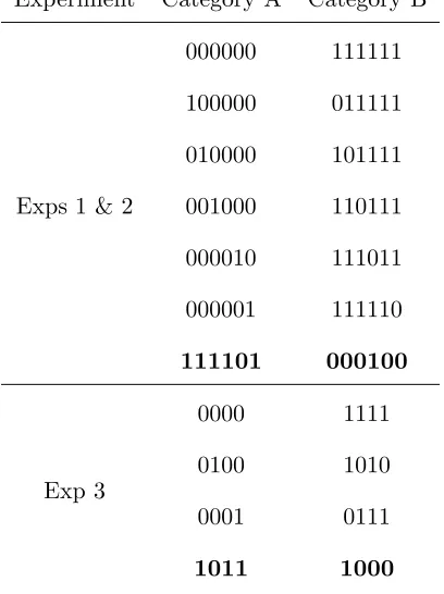
Effect of specific instances

In a classic paper, Medin and Schaffer (1978) tested whether categorization

judgments were influenced by the central tendency of a category alone. In their

Experiment 1, the stimuli were designed so as to test whether the nearness of stimuli had

an effect above contributing to the category center. The stimuli consisted of six training

items, each with five binary features (including the category label, listed last): 11111,

10101, 01011, 00000, 01000, and 10110. In the transfer session, the training items and

additional items were rated. The transfer stimuli are presented in Table 2, ordered by

human category ratings. These transfer stimuli were structured so that some were closer

to specific instances than others, while the distance to the category centers was constant.

In this experiment, an effect of specific instances was found in the ratings.

Anderson (1991) ran the local MAP algorithm for several different values of the

coupling parameter, but with a fixed prior ofβ = 1. The order of the training items was

randomized on each block. Low values of the coupling parameter, such asc= 0.3,

produced high correlations to human ratings (r = 0.87). At such values of the coupling

parameter, the representation tends to be more exemplar-like than prototype-like, which is

consistent with an effect of specific instances. We ran the particle filter algorithm on this

experimental design withM = 100 andM = 1 particles. The particle filter withM = 1

particle was replicated 1,000 times and theM = 100 particle particle filter was replicated

10 times. The results are shown in Figure 8. Using the same coupling parameter, c= 0.3,

we found good correlations for the multi-particle particle filter (r = 0.78) and for the

single-particle particle filter (r = 0.77). We also examined lower values of the coupling

r= 0.88, but the single-particle improved somewhat, tor= 0.84, as did the particle filter

withM = 100 particles (r= 0.84).

Prediction performance and the range of predicted probabilities both increase if the

model is trained with the same number of blocks human subjects were trained (ten)

instead of just a single block. Across coupling parameters, the best correlation with

human ratings were high for the local MAP (r= 0.95), the particle filter withM = 1

particles (r= 0.90), and the particle filter with M = 100 particles (r= 0.93). Overall, the

results in Figure 8 look accurate for all of the models, except for a serious disagreement

between the human data and model predictions for 1110, the seventh stimulus from the

left. Human ratings for 1110 diverged from the ratings of 0111 and 1101, the fourth and

fifth stimuli from the left. However these three stimuli are the same distances from the

training stimuli, so the models tended to give these three stimuli the same probability of

Category 1 as a result.

Specific instances with continuous features

The effect of specific instances has been studied with continuous features in Nosofsky

(1988). In this study, subjects were trained on 12 stimuli that varied in brightness and

saturation. As in Medin and Schaffer (1978), the category structure could not be learned

using only one feature. However, in this experiment, the frequency of specific examples

was manipulated. Over the course of two experiments, subjects showed a sensitivity to the

presentation frequency of specific colors. Anderson (1991) fit the RMC to these data using

a likelihood function (following Gelman, Carlin, Stern, & Rubin, 2004) appropriate for

continuous data. The continuous likelihood used was a Gaussian distribution for each

cluster and the chosen parameters are described in the Appendix. In this simulation, the

values of the continuous dimension prior parameters wereλ0 = 1 anda0 = 1. The label

an overall correlation between the two experiments ofr = 0.98 with the human data.

Both the single-particle particle filter and the particle filter withM = 100 particles

were run with these same parameters. There were 1,000 replications of the single-particle

particle filter and 10 repetitions of theM = 100 particle particle filter. On each

replication, the stimuli were presented in a new random order. The overall correlation

between the human data in the two experiments and the average output of the model was

r= 0.97 for the single-particle particle filter andr = 0.98 forM = 100 particles. Here

again, both types of particle filters perform as well as the local MAP algorithm.

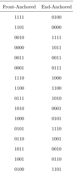
Order effects

Order effects provide a strong challenge to stationary Bayesian models, such as the

statistical model underlying the RMC (Kruschke, 2006a, 2006b). A DPMM by nature does

not produce order effects, because the observations are exchangeable under the model.

However, order effects are easily found in investigations of human cognition, most saliently

in the primacy and recency effects found in free recall of a list of words (Murdock, 1962).

In categorization research, order effects are well established (Medin & Bettger, 1994). We

examine the order effects found including order sensitivity data collected by Anderson and

Matessa (reported in Anderson, 1990) to support the approximation used in the RMC.

The rational model is not able to predict these order effects, but approximations to

the rational model can. Approximations only assign mass to a small portion of the

posterior space over partitions, in effect embodying only a small number of hypotheses

about how the stimuli should be clustered. When a new trial is added to the

representation, the possible new representations are extensions of the previous

representations. So, if a particular partition of the existing stimuli is not present among

the particles, then it will never appear when the representation has been updated. In this