Finding the Most Probable String and the Consensus String: an
Algorithmic Study
Colin de la Higuera∗ and Jose Oncina∗∗
∗Universit´e de Nantes, CNRS, LINA, UMR6241, F-44000, France
∗∗Departamento de Lenguajes y Sistemas Informaticos
Universidad de Alicante, Alicante, Spain
Abstract
The problem of finding the most proba-ble string for a distribution generated by a weighted finite automaton or a probabilistic grammar is related to a number of important questions: computing the distance between two distributions or finding the best transla-tion (the most probable one) given a abilistic finite state transducer. The prob-lem is undecidable with general weights and isN P-hard if the automaton is probabilis-tic. We give a pseudo-polynomial algorithm which computes the most probable string in time polynomial in the inverse of the proba-bility of the most probable string itself, both for probabilistic finite automata and proba-bilistic context-free grammars. We also give a randomised algorithm solving the same problem.
1 Introduction
When using probabilistic machines to define dis-tributions over sets of strings, the usual and best studied problems are those of parsing and of find-ing the most probable explanation of a given string (the most probable parse). These problems, when dealing with probabilistic (generating) finite state automata, hidden Markov Models (HMMs) or probabilistic context-free grammars depend on the ambiguity of the machine: indeed, if there can be different parses for the same string, then the prob-ability of the string is obtained by summing over the different parses.
A more difficult problem we study here is that of finding the most probable string; this string is also known as the consensus string.
The problem of finding the most probable string was first addressed in the computational linguis-tics community by Sima’an (1996): he proved the problem to beN P-hard if we consider tree gram-mars, and as a corollary he gave the same result for
context-free grammars. Goodman (1998) showed that, in the case of HMMs, the problem of finding whether the most most probable string of a given lengthnis at leastpisN P-Complete. Moreover, he points that his technique cannot be applied to show theN P-completeness of the problem when
n is not prespecified because the most probable string can be exponentially long. Casacuberta and de la Higuera (2000) proved the problem to be N P-hard, using techniques developed for lin-guistic decoding (Casacuberta and de la Higuera, 1999): their result holds for probabilistic finite state automata and for probabilistic transducers even when these are acyclic: in the transducer case the related (and possibly more important) ques-tion is that of finding the most probable transla-tion. The problem was also addressed with mo-tivations in bioinformatics by Lyngsø and Peder-sen (2002). Their technique relies on reductions from maximal cliques. As an important corol-lary of their hardness results they prove that the
L1 andL∞distances between distributions
repre-sented by HMMs are also hard to compute: indeed being able to compute such distances would en-able to find (as a side product) the most proben-able string. This result was then applied on probabilis-tic finite automata in (Cortes et al., 2006; Cortes et al., 2007) and theLkdistance, for each oddkwas
proved to be intractable.
An essential consequence of these results is that finding the most probable translation given some probabilistic (non deterministic) finite state trans-ducer is also at least as hard. It can be shown (Casacuberta and de la Higuera, 1999; Vidal et al., 2005) that solving this problem consists in finding the most probable string inside the set of all ac-ceptable translations, and this set is structured as a probabilistic finite automaton. Therefore, the most probable translation problem is alsoN P-hard.
On the other hand, in the framework of multi-plicity automata or of accepting probabilistic finite
automata (also called Rabin automata), the prob-lem of the existence of a string whose weight is above (or under) a specific threshold is known to be undecidable (Blondel and Canterini, 2003). In the case where the weight of each individual edge is between 0 and 1, the score can be interpreted as a probability. The differences reside in the fact that in multiplicity automata the sum of the probabili-ties of all strings does not need to be bounded; this is also the case for Rabin automata, as each prob-ability corresponds to the probprob-ability for a given string to belong to the language.
In this paper we attempt to better understand the status of the problem and provide algorithms which find a string of probability higher than a given threshold in time polynomial in the inverse of this threshold. These algorithms give us prag-matic answers to the consensus string problem as it is possible to use the probabilistic machine to de-fine a threshold and to use our algorithms to find, in this way, the most probable string.
We will first (Section 2) give the different defi-nitions concerning automata theory, distributions over strings and complexity theory. In Section 3 we show that we can compute the most prob-able string in time polynomial in the inverse of the probability of this most probable string but in the bounded case, i.e. when we are looking for a string of length smaller than some given bound. In Section 4 we show how we can compute such bounds. In Section 5 the algorithms are experi-mentally compared and we conclude in Section 6.
2 Definitions and Notations
2.1 Languages and Distributions
Let[n]denote the set{1, . . . , n}for eachn ∈N. An alphabet Σ is a finite non-empty set of sym-bols called letters. A string w over Σ is a fi-nite sequence w = a1. . . an of letters. Let |w|
denote the length of w. In this case we have
|w| = |a1. . . an| = n. The empty string is
denoted by λ. When decomposing a string into substrings, we will write w = w1. . . wn where
∀i∈[n]wi ∈Σ⋆.
Letters will be indicated by a, b, c, . . ., and strings byu, v, . . . , z.
We denote byΣ⋆ the set of all strings, byΣn
the set of those of lengthn, byΣ<n(respectively
Σ≤n, Σ≥n) the set of those of length less than n
(respectively at mostn, at leastn).
A probabilistic languageDis a probability
dis-tribution over Σ⋆. The probability of a string
x ∈ Σ⋆ under the distribution D is denoted as
P rD(x)and must verifyP
x∈Σ⋆P rD(x) = 1.
If the distribution is modelled by some syntactic machineM, the probability ofxaccording to the probability distribution defined by Mis denoted
P rM(x). The distribution modelled by a machine
Mwill be denoted byDM and simplified toDif
the context is not ambiguous.
IfLis a language (thus a set of strings, included inΣ⋆), andDa distribution overΣ⋆,P rD(L) =
P
x∈LP rD(x).
2.2 Probabilistic Finite Automata
The probabilistic finite automata (PFA) (Paz, 1971) are generative devices:
Definition 1. A Probabilistic Finite Automaton (PFA) is a tupleA=hΣ, Q, S, F, δi, where:
- Σis the alphabet;
- Q={q1,. . . ,q|Q|}is a finite set of states;
- S:Q→R+∩[0,1](initial probabilities);
- F :Q→R+∩[0,1](final probabilities);
- δ : Q × (Σ ∪ {λ}) × Q → R+ is a
transition function; the function is complete:
δ(q, a, q′) = 0 can be interpreted as “no transition fromqtoq′ labelled witha”.
S,δandF are functions such that:
X
q∈Q
S(q) = 1, (1)
and∀q∈Q,
F(q) + X
a∈Σ∪{λ}, q′
∈Q
δ(q, a, q′) = 1. (2)
Let x ∈ Σ⋆. Π
A(x) is the set of all
paths accepting x: a path is a sequence π =
qi0x1qi1x2. . . xnqin where x = x1· · ·xn, xi ∈ Σ ∪ {λ}, and ∀j ≤ n, ∃pj 6= 0 such that
δ(qij−1, xj, qij) = pj. The probability of the path
πis
S(qi0)·
Y
j∈[n]
pj·F(qin)
And the probability of the string x is obtained by summing over all the paths in ΠA(x). Note that this may result in an infinite sum because of
An effective computation can be done by means of the Forward (or Backward) algorithm (Vidal et al., 2005).
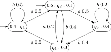
0.4 :q1
0.6 :q2: 0.1
q3: 0.4
q4: 0.3
a0.5 a0.5
b0.4
a0.5
b0.2
b0.5
[image:3.595.85.264.115.199.2]a0.2 b0.4
Figure 1: Graphical representation of a PFA.
Alternatively, a PFA (with n states) is given
when the following matrices are known:
• S ∈ R1×n represents the probabilities of
starting at each state.S[i]=S(qi);
• M = {Ma ∈ Rn×n|a ∈ Σ∪ {λ}}
repre-sents the transition probabilities. Ma[i, j] =
δ(qi, a, qj);
• F ∈ Rn×1 represents the probabilities of
ending in each state.F[i]=F(qi).
Given a string x = a1· · ·ak we compute
P rA(x)as:
P rA(x) =S |x|
Y
i=1
[M∗
λMai]M∗λF (3)
where
M∗ λ=
∞
X
i=0
Mλi = (I−Mλ)−1
Then, equations 1 and 2 can be written as:
S1= 1 (4)
X
a∈Σ∪{λ}
Ma1+F=1 (5)
where1∈Rnis such that∀i1[i] = 1. Note that
P rA(λ) =SM∗
λF∈[0,1] (6)
This implies thatM∗
λ should be a non singular
matrix.
Moreover, in order forP rAto define a distribu-tion probability overΣ⋆it is required that:
X
x∈Σ∗
P rA(x) = ∞
X
i=0
SM∗
λMiΣM∗λF
=SM∗λ(I−MΣ)−1M∗λF= 1
where I is the identity matrix and MΣ =
P
a∈ΣMa. Note that as a consequence of that, (I −MΣ)is a non singular matrix.
2.3 Hidden Markov Models
Hidden Markov models (HMMs) (Rabiner, 1989; Jelinek, 1998) are finite state machines defined by (1) a finite set of states, (2) a probabilistic transi-tion functransi-tion, (3) a distributransi-tion over initial states, and (4) an output function.
An HMM generates a string by visiting (in a hidden way) states and outputting values when in those states. Typical problems include finding the most probable path corresponding to a particular output (usually solved by the Viterbi algorithm). Here the question of finding the most probable output has been addressed by Lyngsø and Peder-sen (2002). In this paper the authors prove that the hardness of this problem implies that it is also hard to compute certain distances between two distribu-tions given by HMMs.
Note that to obtain a distribution over Σ⋆ and not eachΣn the authors introduce a unique final
state in which, once reached, the machine halts. An alternative often used is to introduce a special symbol (♯) and to only consider the strings termi-nating with♯: the distribution is then overΣ⋆♯.
Equivalence results between HMMs and PFA
can be found in (Vidal et al., 2005).
2.4 Probabilistic Context-free Grammars
Definition 2. A probabilistic context-free gram-mar (PCFG) Gis a quintuple< Σ, V, R, P, N > where Σ is a finite alphabet (of terminal sym-bols),V is a finite alphabet (of variables or non-terminals), R ⊂ V × (Σ ∪ V)∗ is a finite set of production rules, and N (∈ V) is the axiom.
P :R→R+is the probability function.
A PCFGis used to generate strings by rewriting
Particularly appealing is a very efficient exten-sion of the Early algorithm due to Stolcke (1995) that can compute:
• the probability of a given string xgenerated by a PCFGG;
• the single most probable parse forx;
• the probability that x occurs as a prefix of some string generated byG, which we denote byP rG(xΣ⋆).
2.5 Probabilistic Transducers
There can be different definitions of probabilistic transducers. We use the one from (Vidal et al., 2005):
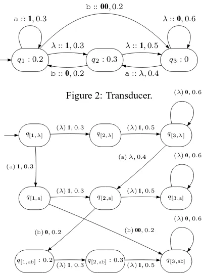
q1: 0.2 q2: 0.3 q3: 0
λ::1,0.3
b::00,0.2
b::0,0.2
λ::1,0.5
a::λ,0.4
[image:4.595.313.528.49.165.2]a::1,0.3 λ::0,0.6
Figure 2: Transducer.
q[1,λ] q[2,λ] q[3,λ]
q[1,a] q[2,a] q[3,a]
q[1,ab]: 0.2 q[2,ab]: 0.3 q[3,ab] (λ)1,0.3 (λ)1,0.5
(λ)0,0.6
(a)1,0.3
(a)λ,0.4
(λ)1,0.3 (λ)1,0.5
(λ)0,0.6
(b)00,0.2 (b)0,0.2
(λ)1,0.3 (λ)1,0.5
(λ)0,0.6
Figure 3: Corresponding non normalized PFA for the translations of ab. Each state indicates which input prefix has been read. Between the brackets, on the tran-sitions, the input symbol justifying the transition.
Probabilistic finite-state transducers (PFST) are similar to PFA, but in this case two different
alpha-bets (source Σand target Γ) are involved. Each transition in a PFST has attached a symbol from the source alphabet (or λ) and a string (possible empty string) of symbols from the target alphabet. PFSTs can be viewed as graphs, as for example in Figure 3.
Definition 3 (Probabilistic transducer). A proba-bilistic finite state transducer (PFST) is a 6-tuple
hQ,Σ,Γ, S, E, Fisuch that:
q1,λ q3,λ q3,λ
q1,a q2,a
q1,ab: 0.4 q2,ab: 1
1,0.5 1,1 0,0.6
1,0.5
λ,0.4
1,1
0,1
1,0.6
Figure 4: Corresponding normalized PFAfor the trans-lations ofab. The most probable string (111) has prob-ability 0.54.
- Q is a finite set of states; these will be la-belledq1,. . . ,q|Q|;
- S:Q→R+∩[0,1](initial probabilities);
- F :Q→R+∩[0,1](halting probabilities);
- E∈Q×(Σ∪ {λ})×Γ⋆×Q×R+is the set of transitions;
S,δandF are functions such that:
X
q∈Q
S(q) = 1,
and∀q ∈Q,
F(q) + X
a∈Σ∪{λ}, q′
∈Q
p: (q, a, w, q′, p)∈E = 1.
Let x ∈ Σ⋆ andy ∈ Γ⋆. LetΠT(x, y) be the set of all paths accepting (x, y): a path is a se-quence π = qi0(x1, y1)qi1(x2, y2). . .(xn, yn)qin
wherex=x1· · ·xnandy=y1· · ·yn, with∀j ∈
[n], xj ∈Σ∪{λ}andyj ∈Γ⋆, and∀j∈[n],∃pij
such that (qij−1, xj, yj, qij, pij) ∈ E. The
proba-bility of the path is
S(qi0)·
Y
j∈[n]
pij·F(qin)
And the probability of the translation pair (x, y)
is obtained by summing over all the paths in
ΠT(x, y).
Note that the probability of y given x (the probability of y as a translation of x, denoted as
P rT(y|x)) is P rT(x,y)
P
z∈Σ⋆P rT(x,z).
Probabilistic finite state transducers are used as models for the the stochastic translation problem of a source sentencex∈Σ⋆that can be defined as
the search for a target stringythat:
argmax y
P r(y|x) = argmax y
[image:4.595.73.273.279.549.2]The problem of finding this optimal translation is proved to be aN P-hard by Casacuberta and de la Higuera (2000).
An approximate solution to the stochastic trans-lation can be computed in polynomial time by us-ing an algorithm similar to the Viterbi algorithm for probabilistic finite-state automata (Casacu-berta, 1995; Pic´o and Casacu(Casacu-berta, 2001).
The stochastic translation problem is compu-tationally tractable in particular cases. If the PFSTT is non-ambiguous in the translation sense
(∀x ∈ Σ⋆ there are not two target sentences
y, y′ ∈ Γ⋆,y 6=y′, such thatP rT(x, y) > 0and
P rT(x, y′) >0), the translation problem is poly-nomial. If the PFST T is simply non-ambiguous (∀x ∈ Σ⋆ there are not two different paths that deal with (x, y) and with probability different to zero), the translation problem is also polynomial. In both cases, the computation can be carried out using an adequate version of the Viterbi algorithm (Vidal et al., 2005).
Alternative types of PFSTs have been intro-duced and applied with success in different areas of machine translation. In (Mohri, 1997; Mohri et al., 2000), weighted finite-state transducers are studied.
2.6 Complexity Classes and Decision Problems
We only give here some basic definitions and re-sults from complexity theory. A decision
prob-lem is one whose answer is true or false. A
deci-sion problem is decidable if there is an algorithm which, given any specific instance, computes cor-rectly the answer and halts. It is undecidable if not. A decision problem is inP if there is a poly-nomial time algorithm that solves it.
A decision problem isN P-complete if it is both
N P-hard and in the class N P: in this case a polynomial time non-deterministic algorithm ex-ists that always solves this problem. Alterna-tively, a problem is inN P if there exists a
poly-nomial certificate for it. A polypoly-nomial certificate
for an instance I is a short (polynomial length) string which when associated to instanceI can be checked in polynomial time to confirm that the in-stance is indeed positive. A problem isN P-hard if it is at least as hard as the satisfiability problem (SAT), or either of the other N P-complete prob-lems (Garey and Johnson, 1979).
A randomized algorithm makes use of random
bits to solve a problem. It solves a decision
prob-lem with one-sided error if given any valueδ and any instance, the algorithm:
• makes no error on a negative instance of a problem (it always answers no);
• makes an error in at mostδcases when work-ing on a positive instance.
If such an algorithm exists, the problem is said to belong to the classRP. It should be noticed that by running such a randomized algorithmntimes the error decreases exponentially withn: if a pos-itive answer is obtained, then the instance had to be positive, and the probability of not obtaining a positive answer (for a positive instance) inntries is less than δn. A randomized algorithm which solve a decision problem in the conditions above is called a Monte Carlo algorithm.
When a decision problem depends on an in-stance containing integer numbers, the fair (and logical) encoding is in base 2. If the problem ad-mits a polynomial algorithm whenever the integers are encoded in base 1, the problem (and the algo-rithm) are said to be pseudo-polynomial.
2.7 About Sampling
One advantage of using PFAor similar devices is that they can be effectively used to develop domised algorithms. But when generating ran-dom strings, the fact that the length of these is un-bounded is an issue. Therefore the termination of the algorithm might only be true with probability
1: this means that the probability of an infinite run,
even if it cannot be discarded, is of null measure. In the work of Ben-David et al. (1992) which extends Levin’s original definitions from (Levin, 1986), a distribution over {0,1}∗ is considered samplable if it is generated by a randomized
al-gorithm that runs in time polynomial in the length of its output.
We will require a stronger condition to be met. We want a distribution represented by some ma-chine M to be sampable in a bounded way, ie, we require that there is a randomized algorithm which, when given a bound b, will either return any stringwinΣ≤b with probabilityP rM(w)or return fail with probability P rM(Σ>b). Further-more, the algorithm should run in time polynomial inb.
sampable if
• one can parse an input string x by M and returnP rM(x)in time polynomial in|x|;
• one can sampleDMin a bounded way.
2.8 The Problem
The question is to find the most probable string in a probabilistic language. An alternative name to this string is the consensus string.
Name: Consensus string (CS)
Instance: A probabilistic machineM
Question: Find in Σ⋆ a string x such that
∀y∈ Σ⋆ P rM(x)≥P rM(y).
With the above problem we associate the fol-lowing decision problem:
Name: Most probable string (MPS)
Instance: A probabilistic machineM, ap≥0
Question: Is there in Σ⋆ a string x such that
P rM(x)≥p?
For example, if we consider the PFAfrom Fig-ure 1, the most probable string isa.
Note thatpis typically encoded as a fraction and that the complexity of our algorithms is to depend on the size of the encodings, hence oflog1p.
The problem MPS is known to be N P-hard (Casacuberta and de la Higuera, 2000). In their proof the reduction is from SAT and uses only
acyclic PFA. There is a problem with MPS: there is no bound, in general, over the length of the most probable string. Indeed, even for regular lan-guages, this string can be very long. In Section 4.4 such a construction is presented.
Of interest, therefore, is to study the case where the longest string can be bounded, with a bound given as a separate argument to the problem:
Name: Bounded most probable string (BMPS) Instance: A probabilistic machine M, ap ≥ 0, an integerb
Question: Is there in Σ≤b a string x such that
P rM(x)≥p?
In complexity theory, numbers are to be en-coded in base 2. In BMPS, it is necessary, for the
problem not to be trivially unsolvable, to consider a unary encoding ofb, as strings of length up tob
will have to be built.
3 Solving BMPS
In this section we attempt to solve the bounded case. We first solve it in a randomised way, then propose an algorithm that will work each time the prefix probabilities can be computed. This is the case for PFAand for probabilistic context free grammars.
3.1 Solving by Sampling
Let us consider a class of strongly sampable ma-chines.
Then BMPS, for this class, belongs toRP:
Theorem 1. If a machineMis strongly sampable,
BMPScan be solved by a Monte Carlo algorithm.
Proof. The idea is that any stringswhose proba-bility is at leastp, should appear (with high proba-bility, at least1−δ) in a sufficiently large randomly drawn sample (of sizem), and have a relative fre-quency mf of at least p2.
Algorithm 1 therefore draws this large enough sample in a bounded way and then checks if any of the more frequent strings (relative frequencymf of at least p2) has real probability at leastp.
We use multiplicative Chernov bounds to com-pute the probability that an arbitrary string whose probability is at least p has relative frequency mf of at least p2:
P r f
m < p
2
≤2e−mp/8
So for a value of δ ≤ 2e−mp/8 it is sufficient to draw a sample of sizem ≥ 8pln2δ in order to be certain (with errorδ) that in a sample of sizem
any probable string is in the sample with relative frequency mf of at least p2.
We then only have to parse each string in the sample which has relative frequency at least p2 to be sure (within errorδ) thatsis in the sample.
If there is no string with probability at least p, the algorithm will return false.
The complexity of the algorithm depends on that of bounded sampling and of parsing. One can check that in the case of PFA, the generation is in
O(b·log|Σ|)and the parsing (of a string of length at mostb) is inO(b· |Q|2).
3.2 A Direct Computation in the Case of PFA
Data: a machineM,p≥0,b≥0
Result: w∈Σ≤bsuch thatP r
M(w)≥p,
false if there is no suchw
begin Mapf;
m= 8pln2δ; repeat mtimes
w=bounded sample(M, b); f[w]++;
foreachw:f[w]≥ pm2 do if PrM(w)≥pthen
returnw;
return false
Algorithm 1: Solving BMPS in the general
case
We are given ap > 0 and a PFAA. Then we have the following properties:
Property 1. ∀u∈Σ⋆,P rA(uΣ⋆)≥P rA(u).
Property 2. For eachn ≥ 0there are at most 1p stringsuinΣnsuch thatP rA(uΣ⋆)≥p.
Both proofs are straightforward and hold not only for PFAbut for all distributions. Notice that a stronger version of Property 2 is Property 3:
Property 3. IfX is a set of strings such that (1)
∀u ∈ X, P rA(uΣ⋆) ≥ p and (2) no string inX is a prefix of another different string in X, then
|X| ≤ 1p.
Analysis and complexity of Algorithm 2. The idea of the algorithm is as follows. For each length
n compute the set of viable prefixes of lengthn, and keep those whose probability is at leastp. The process goes on until either there are no more vi-able prefixes or a valid string has been found. We use the fact thatP rA(uaΣ⋆)andP rA(u)can be computed from P rA(uΣ⋆) provided we
memo-rize the value in each state (by a standard dynamic programming technique). Property 2 ensures that at every moment at most 1p valid prefixes are open. If all arithmetic operations are in constant time, the complexity of the algorithm is inO(b|Σ|·|pQ|2).
3.3 Sampling Vs Exact Computing
BMPScan be solved with a randomized algorithm (and with error at mostδ) or by the direct Algo-rithm 2. If we compare costs, and assuming that bounded sampling a string can be done in time linear inb, and that all arithmetic operations take constant time we have:
Data: a PFA:A=hΣ,S,M,Fi,p≥0,
b≥0
Result: w∈Σ≤bsuch thatP r
A(u)≥p,
false if there is no suchw
begin
QueueQ;
pλ =SF;
if pλ ≥pthen
returnpλ;
push(Q, (λ,F)); while notempty(Q)do
(w,V) =pop(Q); foreach a∈Σdo
V′ =VMa;
if V′F≥pthen returnV′F;
if |w|< bandV′1≥pthen push(Q, (wa,V′));
return false
Algorithm 2: Solving BMPSfor automata
• Complexity of (randomized) Algorithm 1 for PFAis inO(8pbln2δ·log|Σ|)to build the sam-ple andO(2pb· |Q|2)to check the 2p most fre-quent strings.
• Complexity of Algorithm 2 is inO(b|Σ|·|pQ|2). Therefore,for the randomized algorithm to be faster, the alphabet has to be very large. Experi-ments (see Section 5) show that this is rarely the case.
3.4 Generalising to Other Machines
What is really important in Algorithm 2 is that the differentP rM(uΣ⋆)can be computed. If this is
a case, the algorithm can be generalized and will work with other types of machines. This is the case for context-free grammars (Stolcke, 1995).
For classes which are strongly sampable, we propose the more general Algorithm 3.
4 More about the Bounds
The question we now have to answer is: how do we choose the bound? We are given some machine
M and a number p ≥ 0. We are looking for a value np which is the smallest integer such that
P rM(x)≥p =⇒ |x| ≤ np. If we can compute
Data: a machineM,p≥0,b≥0
Result: w∈Σ≤bsuch thatP r
M(w)≥p,
false if there is no suchw
begin
QueueQ;
pw =P rM(λ);
if pw ≥pthen returnpw;
push(Q,λ);
while notempty(Q)do
w=pop(Q); foreach a∈Σdo
if P rM(wa)≥pthen returnP rM(wa);
if |w|< bandP rM(waΣ∗)≥p
then
push(Q,wa);
return false
Algorithm 3: Solving BMPS for general ma-chines
4.1 Computing Analyticallynp
If given the machineMwe can compute the mean
µ and the varianceσ of the length of strings in
DM, we can use Chebychev’s inequality:
P rM |x| −µ > kσ
< 1
k2
We now choosek= √1p and rewrite:
P rM |x|> µ+√σ
p
< p
This means that, if we are looking for strings with a probability bigger than p, it is not necessary to consider strings longer thanµ+√σp.
In other words, we can setb=⌈µ+√σp⌉and run an algorithm from Section 3 which solves BMPS.
4.2 Computing Analyticallynpfor PFA
We consider the special case where the probabilis-tic machine is a PFA A. We are interested in computing the mean and the variance of the string length. It can be noted that the fact the PFAis de-terministic or not is not a problem.
The mean string length of the strings generated
byAcan be computed as:
µ=
∞
X
i=0
i P rA(Σi)
= ∞
X
i=0
iSM∗
λMiΣM∗λF
=SM∗λMΣ(I−MΣ)−2M∗λF
Moreover, taking into account that:
∞
X
i=0
i2P rA(Σi) = ∞
X
i=0
i2SM∗λMiΣM∗λF
=SM∗λMΣ(I+MΣ)(I−MΣ)−3M∗λF
The variance can be computed as:
σ2= ∞
X
i=0
(i−µ)2P rA(Σi)
= ∞
X
i=0
i2P rA(Σi)−µ2
=SM∗
λMΣ(I+MΣ)(I−MΣ)−3M∗λF
−
SM∗λMΣ(I−MΣ)−2M∗λF2
Then, both values are finite since (I −MΣ) is
non singular.
4.3 Computingnp,δvia Sampling
In certain cases we cannot draw an analytically ob-tained value for the mean and the variance. We have to resort to sampling in order to compute an estimation ofnp.
A sufficiently large sample is built and used by Lemma 1 to obtain our result. In that case we have the following:
• If the instance is negative, it is anyhow im-possible to find a string with high enough probability, so the answer will always be false.
• If the instance is positive, the bound returned by the sampling will be good in all but a small fraction (less thanδ) of cases. When the sam-pling has gone correctly, then the algorithm when it halts has checked all the strings up to lengthn. And the total weight of the remain-ing strremain-ings is less thanp.
DM and a positive value p, an integernp,δ such
thatP rDM(Σ
np,δ)< p. If we do this by sampling
we will of course have the result depend also on the valueδ covering the case where the sampling process went abnormally wrong.
Lemma 1. LetDbe a distribution overΣ⋆. Then if we draw, following distribution D, a sampleS
of size at least 1pln1δ, given any p > 0 and any
δ >0, the following holds with probability at least 1-δ: the probability of sampling a stringxlonger than any string seen inSis less thanp.
Alternatively, if we write nS = max{|y| :
y ∈ S}, then, with probability at least 1 − δ,
P rD(|x|> nS)< p.
Proof. Denote by mp the smallest integer such
that the probability for a randomly drawn string to be longer thanmp is less thanp: P rD(Σ>mp) <
p.
We need now to compute a large enough sample to be sure (with a possible error of at mostδ) that
max{|y|:y∈ S} ≥mp. ForP rD(|x|> mp) <
p to hold, a sufficient condition is that we take a sample large enough to be nearly sure (i.e. with probability at least1−δ) to have at least one string as long as mp. On the contrary, the probability
of having all (k) strings in S of length less than
mp is at most(1−p)k. Using the fact that(1−
p)k > δimplies thatk > 1pln1δ, it follows that it is sufficient, once we have chosenδ, to takenp,δ>
1
pln1δ to have a correct value.
Note that in the above, all we ask is that we are able to sample. This is indeed the case with HMM, PFA and (well defined) probablistic
context-free grammars, provided these are not ex-pansive. Lemma 1 therefore holds for any of such machines.
4.4 The Most Probable String Can Be of Exponential Length
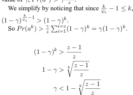
If the most probable string can be very long, how long might it be? We show now an automaton for which the most probable string is of exponential length with the size of the automaton. The con-struction is based on (de la Higuera, 1997). Let us use a value γ > 0whose exact value we will compute later.
We first note (Figure 5) how to build an automa-ton that only gives non null probabilities to strings whose length are multiples ofψfor any value ofψ
(and of particular interest are the prime numbers). Here,P r(akψ) =γ(1−γ)k.
γ
a: 1 a: 1
a: 1
a: 1
[image:9.595.305.525.448.605.2]a: 1−γ
Figure 5: Automaton for(a5
)∗.
We now extend this construction by building for a set of prime numbers { ψ1, ψ2,. . . , ψz}
the automaton for each ψi and adding an initial
state. When parsing a non empty string, a sub-automaton will only add to the mass of probabili-ties if the string is of length multiple ofψi. This
PFA can be constructed as proposed in Figure 6, and has1 +Pi=z
i=1ψistates.
The probability of string ak withk = Qi=z
i=1pi isPi=z
i=11zγ(1−γ) k ψi−1= γ
z
Pi=z
i=1(1−γ)
k ψi−1.
First consider a string of length less thank. This string is not accepted by at least one of the sub-automata so it’s probability is at mostγz−z1.
On the other hand we prove now that for a good value ofγ,P r(ak)> γz−z1.
We simplify by noticing that since ψk
i −1≤k, (1−γ)
k
ψi−1 >(1−γ)k.
SoP r(ak)> γzPi=z
i=1(1−γ)k=γ(1−γ)k.
(1−γ)k> z−1 z
1−γ > k r
z−1
z
γ <1− k
r z−1
z
no shorter string can have higher probability.
5 Experiments
We report here some experiments in which we compared both algorithms over probabilistic au-tomata.
γ
a: 1 a: 1
a: 1
a: 1 a: 1−γ
γ
a: 1 a: 1−γ
γ a: 1
a: 1
a: 1−γ a:1z
a:1
z
a:1z
γ a:1z
[image:10.595.89.274.81.265.2]γ a:1z
Figure 6: An automaton whose smallest ‘interesting string’ is of exponential length.
previous states labelled by all the symbols of the vocabulary.
The probabilities on the edges and the final state were set assigning to them randomly (uniformly) distributed numbers in the range [0,1] and then normalizing.
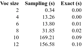
Voc size Sampling (s) Exact (s)
2 0.34 0.00
4 13.26 0.00
6 13.80 0.01
8 31.85 0.02
10 169.21 0.09
12 156.58 0.10
Table 1: Execution time of Algorithm 1 (sampling) and Algorithm 2 (exact) for 4 state automata
In our experiments, the exact algorithm is sys-tematically faster than the one that uses sampling. Alternative settings which would be favourable to the randomized algorithm are still to be found.
6 Conclusion
We have proved the following:
1. There exists a PFA whose most probable string is not of polynomial length.
2. If we can sample and parse (strongly sam-pable distribution), then we have a ran-domised algorithm which solves MPS.
3. If furthermore we can analytically compute the mean and variance of the distribution, there is an exact algorithm for MPS. This means that the problem is decidable for a PFA
or HMMs.
4. In the case of PFAthe mean and the variance are polynomially computable, so MPScan be solved in time polynomial in the size of the PFAand in 1p.
5. In the case of PFA, we can use practical
algo-rithms:
(a) randomly draw a sampleS ofnstrings following distributionDA;
(b) let p = max{p(u) : u ∈ S} andb = max{|u|:u∈S};
(c) run Algorithm 2 usingpandb.
Practically, the crucial problem may be CS; A consensus string can be found by either sampling to obtain a lower bound to the probability of the most probable string and solving MPS, or by some form of binary search.
Further experiments are needed to see in what cases the sampling algorithm works better, and also to check its robustness with more complex models (like probabilistic context-free grammars). Finally, in Section 4.4 we showed that the length of the most probable string could be exponential, but it is unclear if a higher bound to the length can be obtained.
Acknowledgement
Discussions with Pascal Koiran during earlier stages of this work were of great help towards the understanding of the nature of the problem. The first author also acknowledges partial support by the R´egion des Pays de la Loire. The sec-ond author thanks the Spanish CICyT for partial support of this work through projects TIN2009-14205-C04-C1, and the program CONSOLIDER
[image:10.595.101.264.424.521.2]References
S. Ben-David, B. Chor, O. Goldreich, and M. Luby. 1992. On the theory of average case complexity. Journal of Computer and System
Sciences, 44(2):193—-219.
V. D. Blondel and V. Canterini. 2003. Unde-cidable problems for probabilistic automata of fixed dimension. Theory of Computer Systems, 36(3):231–245.
F. Casacuberta and C. de la Higuera. 1999. Op-timal linguistic decoding is a difficult compu-tational problem. Pattern Recognition Letters, 20(8):813–821.
F. Casacuberta and C. de la Higuera. 2000. Com-putational complexity of problems on proba-bilistic grammars and transducers. In
Proceed-ings of ICGI2000, volume 1891 of LNAI, pages 15–24. Springer-Verlag.
F. Casacuberta. 1995. Probabilistic estimation of stochastic regular syntax-directed translation schemes. In R. Moreno, editor, VI Spanish
Sym-posium on Pattern Recognition and Image Anal-ysis, pages 201–297. AERFAI.
C. Cortes, M. Mohri, and A. Rastogi. 2006. On the computation of some standard distances be-tween probabilistic automata. In Proceedings
of CIAA 2006, volume 4094 of LNCS, pages 137–149. Springer-Verlag.
C. Cortes, M. Mohri, and A. Rastogi. 2007. lp dis-tance and equivalence of probabilistic automata.
International Journal of Foundations of Com-puter Science, 18(4):761–779.
C. de la Higuera. 1997. Characteristic sets for polynomial grammatical inference. Machine Learning Journal, 27:125–138.
M. R. Garey and D. S. Johnson. 1979. Computers
and Intractability. Freeman.
Joshua T. Goodman. 1998. Parsing Inside–Out. Ph.D. thesis, Harvard University.
F. Jelinek. 1998. Statistical Methods for Speech
Recognition. The MITPress, Cambridge, Mas-sachusetts.
L. Levin. 1986. Average case complete problems.
SIAM Journal on Computing, 15(1):285–286.
R. B. Lyngsø and C. N. S. Pedersen. 2002. The consensus string problem and the complexity of comparing hidden markov models. Journal of
Computing and System Science, 65(3):545–569.
M. Mohri, F. C. N. Pereira, and M. Riley. 2000. The design principles of a weighted finite-state transducer library. Theoretical Computer
Sci-ence, 231(1):17–32.
M. Mohri. 1997. Finite-state transducers in lan-guage and speech processing. Computational
Linguistics, 23(3):269–311.
A. Paz. 1971. Introduction to probabilistic
au-tomata. Academic Press, New York.
D. Pic´o and F. Casacuberta. 2001. Some statistical-estimation methods for stochastic finite-state transducers. Machine Learning Journal, 44(1):121–141.
L. Rabiner. 1989. A tutorial on hidden Markov models and selected applications in speech recoginition. Proceedings of the IEEE, 77:257– 286.
K. Sima’an. 1996. Computational complexity of probabilistic disambiguation by means of tree-grammars. In COLING, pages 1175–1180.
A. Stolcke. 1995. An efficient probablistic context-free parsing algorithm that computes prefix probabilities. Computational Linguistics, 21(2):165–201.