The Response to Arbitrarily Bandlimited Gaussian Noise of the Complex Stretch Processor Using a Conventional Range Sidelobe Reduction Window

(1)

http://www.scirp.org/journal/jsip ISSN Online: 2159-4481 ISSN Print: 2159-4465

DOI: 10.4236/jsip.2018.91003 Feb. 13, 2018 36 Journal of Signal and Information Processing

The Response to Arbitrarily Bandlimited

Gaussian Noise of the Complex Stretch

Processor Using a Conventional

Range-Sidelobe-Reduction Window

John N. Spitzmiller

Simulation & Integration Services, Parsons Government Services, Inc., Huntsville, AL, USA

Abstract

This paper derives a mathematical description of the complex stretch proces-sor’s response to bandlimited Gaussian noise having arbitrary center fre-quency and bandwidth. The description of the complex stretch processor’s random output comprises highly accurate closed-form approximations for the probability density function and the autocorrelation function. The solution supports the complex stretch processor’s usage of any conventional range- sidelobe-reduction window. The paper then identifies two practical applica-tions of the derived description. Digital-simulation results for the two identi-fied applications, assuming the complex stretch processor uses the rectangu-lar, Hamming, Blackman, or Kaiser window, verify the derivation’s correct-ness through favorable comparison to the theoretically predicted behavior.

Keywords

Stretch Processing, Noise Jamming, Bandlimited Gaussian Noise, Range-Sidelobe-Reduction Windows

1. Introduction

Stretch processing [1]-[6] in radar uses relatively narrowband techniques to process wideband pulses with linear frequency modulation (LFM). Basic stretch processing [2] [3] (i.e., with no range-sidelobe-reduction window) yields the same fine range resolution and the same relatively high range-sidelobe levels produced by matched filtering. To reduce the range-sidelobe levels produced by basic stretch processing of LFM pulses, a practical stretch processor may apply a

How to cite this paper: Spitzmiller, J.N. (2018) The Response to Arbitrarily Band- limited Gaussian Noise of the Complex Stretch Processor Using a Conventional Range-Sidelobe-Reduction Window. Jour-nal of SigJour-nal and Information Processing, 9, 36-62.

https://doi.org/10.4236/jsip.2018.91003

Received: October 31, 2017 Accepted: February 9, 2018 Published: February 13, 2018

http://creativecommons.org/licenses/by/4.0/

(2)

DOI: 10.4236/jsip.2018.91003 37 Journal of Signal and Information Processing multiplicative window (e.g., a Hamming window) prior to the final Fourier- analysis stage [4] [5] [6].

Radar texts addressing noise in stretch processors [3] [4] typically consider only the case of broadband noise (e.g., receiver thermal noise). References [7] and [8] respectively characterized the response to bandlimited Gaussian noise (BLGN) having arbitrary center frequency and bandwidth of the complex stretch processor having no range-sidelobe-reduction window and the complex stretch processor employing a Hamming or Hann window. This paper extends the work in [7] [8] to characterize the output noise’s probability density function (PDF) and autocorrelation function when the complex stretch processor uses any con-ventional multiplicative window to reduce the range-sidelobe levels. The output noise’s PDF and autocorrelation function provide sufficient information for high-fidelity simulation of the complex stretch processor’s output noise via standard techniques. Since the complex stretch processor is a linear system, a radar modeler may simply add the simulated noise to the complex stretch pro-cessor’s simulated response to targets and clutter.

The derivation assumes the BLGN has arbitrary center frequency and band-width. Therefore, the results can describe the output noise due to input receiver thermal noise, broadband-noise jamming, spot-noise jamming, or even spec-trally offset narrowband interference. The paper specifies a mathematical form for the window which can exactly represent the commonly used rectangular, Hamming, Hann, and Blackman windows and can closely approximate all other conventional windows.

Section 2 firstly specifies a simplified functional model of a radar employing a complex stretch processor with a range-sidelobe-reduction window. Section 2 then describes the processor’s response to target-return signals. Section 3 derives a mathematical description, comprising the PDF and the autocorrelation func-tion, of the complex stretch processor’s theoretical response to arbitrarily bandlimited Gaussian noise. Section 4 presents simulation results which verify the derived expressions for two practical applications. Section 5 summarizes the technical approach, presents key findings, and suggests additional research.

2. Review of Complex Stretch Processing

This section reviews the fundamental operations of a radar using complex stretch processing. Figure 1 shows a simplified block diagram of the basic func-tional elements of a monostatic, pulsed radar employing complex stretch processing. This section’s discussion uses the mathematical notation shown in Figure 1 which pictorially represents the complex stretch processor’s stimula-tion by a target-return signal. For analytical convenience we assume the complex stretch processor comprises exclusively continuous-time (CT) subsystems.

2.1. Transmitted Signal

(3)

[image:3.595.228.529.64.188.2]

DOI: 10.4236/jsip.2018.91003 38 Journal of Signal and Information Processing

Figure 1. Block diagram of monostatic radar using complex stretch processing.

( )

cos 2π

( )

(

)

,

T T RF i p

s t =A _ f t+ ∆φ t _Π tτ (1) where AT is the pulse amplitude in volts, fRF is the center radio frequency (RF) in hertz, t is time in seconds,

τ

p is the pulse duration in seconds, and

( )

i t

φ

∆ _{is the instantaneous phase deviation in radians, to the transmit antenna.}

The transmit antenna radiates the pulse to a stationary point target at a slant range R meters from the radar. In Equation (1)

( )

1, 1 2

0, otherwise x

x  ≤

Π _{= }



(2)

is the dimensionless unit-pulse function, and

( )

2π

( )

d

t

i t fi

φ β β

−∞

∆ =

_∫

∆ ₍₃₎

where, for an up-chirped LFM pulse with sweep bandwidth B hertz,

( )

(

) ( )

i p p

f t Bτ t tτ

∆ = Π (4) is the transmitted pulse’s instantaneous frequency deviation in hertz. We substi-tute Equation (4) into Equation (3) and evaluate for Equation (1) to obtain

( )

(

2 2

)

( )

cos 2π π 4 .

T T RF p p p

s t =A _ f t+ B t −τ τ _Π t τ

(5)

2.2. Received Signal

The stationary point target instantaneously reradiates the incident pulse, so the receive antenna produces the voltage signal

( ) (

) (

)

(

)

{

2 ₂

}

(

)

cos 2π 2π π 4 .

R R T T d

R RF RF d d p p d p

s t A A s t

A f t f B t t

τ

τ τ τ τ τ τ

= −

  _ _

= − + _ − − _ Π_ − _ (6)

In Equation (6)

2

d R c

τ =

₍₇₎

is the round-trip propagation delay, and c is the speed of light. The

ra-dar-range equation [9] determines the dimensionless ratio AR AT .

2.3. Quadrature Demodulator’s Output

(4)

DOI: 10.4236/jsip.2018.91003 39 Journal of Signal and Information Processing [10] produces the complex envelope

( )

( ) (

)

{

( )

(

)

}

{

_2π _π 2 _2π _π 2 _π ₄

}

₍

₎

2 cos 2π 2 sin 2π

e RF d p d p d p p .

QD R RF R RF

j f Bt B t B B

R d p

s t LPF s t f t j LPF s t f t

A − τ + τ − τ τ + τ τ − τ t τ τ

= _ _+ _− _

 

= Π_ − _ (8)

In Equation (8) LPF

( )

• indicates the operation of an ideal lowpass filter hav-ing a dimensionless passband gain of unity and a cutoff frequency between B 2 and 2fRF−B 2. Thus, the quadrature demodulator’s output has units of volts.

2.4. Complex Multiplier’s Output

Assuming the stretch processor considers target slant ranges from Rmin to max

R , the slant ranges on this interval correspond to round-trip propagation delays

from

2 min Rmin c

τ = (9) to

2 .

max Rmax c

τ =

₍₁₀₎

To support processing on slant ranges from Rmin to Rmax, the complex multiplier of Figure 1 multiplies sQD

( )

t with the dimensionless complex signal

( )

( ) ( )

M ,

p t =w t x t (11) where

( )

_ej M( )t

(

)

M avg M

x t = ∆φ Π_t−τ T _

(12) is a complex heterodyne signal and w t

( )

is a sidelobe-reduction window. In

Equation (12)

(

)

2 ,

avg min max

τ

=

τ

+

τ

₍₁₃₎

,

M max min p

T

=

τ

−

τ

+

τ

(14)

and

( )

(

_π 2 _2π _π 2 ₄ _π 2

)

_.

M t Bt B avgt BTM B avg p

φ τ τ τ

∆ = − + + −

(15)

Note that Equation (15) is the instantaneous phase deviation corresponding to the instantaneous frequency deviation

( )

(

)(

) (

)

M p avg avg M

f t Bτ t τ t τ T 

∆ = − − Π_ − _

₍₁₆₎

which sweeps down through a bandwidth of

.

M M p

B

=

BT

τ

>

B

(17) Thus,

( )

(

)

2 2

2 2π π π

π

4

e .

avg M avg

p p p p

B BT B

B

j t t

M avg M

x t t T

τ τ

τ τ τ τ

τ

 

− + + − 

 

   

= Π_ − _

₍₁₈₎

(5)

( )

p

( )

(

avg

)

M ,

w t =w t Π_ t−τ T _ (19) where

( )

, 2 2

p avg M avg M

w t =w t τ −T ≤ ≤t τ +T (20)

and wp

( )

t can have any form outside τavg –TM 2≤ ≤t τavg+TM 2.

Equation (18) and Equation (19) have the common time-limiting factor

(

t τavg

)

TM

 

Π_ − __{whose nonzero portion always fully overlaps the nonzero}

portion of Π

(

t−τd

)

τp in Equation (8). We can therefore express the

com-plex multiplier’s output voltage signal as

( )

( ) ( )

( )

₍

₎

_{( )}

2π

e avg d p ,

CM QD p M QD

j B t

R d p p

s t p t s t w t x t s t

A  τ −τ τ +θ t τ τ w t

= =

 

= Π_ − _ (21)

where

(

2 2

)

2 π π

π ₂_π _.

4 4

avg d p

M

RF d

p p

B B

BT

f

τ τ τ

θ τ

τ τ

−

= − − −

(22)

Assuming

( )

2π

e j ftd

p p

W f w t t

∞

−

−∞

=

_∫

₍₂₃₎

exists, the Fourier transform of Equation (21), having units of volt∙seconds or volts/hertz, is

( )

2π ( )

{

(

)

}

e e avg d p dsinc ,

CM

j f B

j

R p p p avg d p

S f

Aτ θW f −  − τ −τ τ τ τ f B τ τ τ 

= ∗ _ − − _ (24)

where ∗ in Equation (24) denotes linear convolution. Thus, we desire a mathematical form for wp

( )

t which equals w t

( )

on

2 2

avg TM t avg TM

τ − ≤ ≤τ + _{and has a convenient Fourier transform. The}

pe-riodic extension of w t

( )

outside τavg−TM 2≤ ≤t τavg+TM 2 satisfies these two criteria. Mathematically,

( )

(

)

.

p M

k

w t w t kT

∞

=−∞

=

∑

− (25) Since this wp

( )

t is periodic with period TM, we can express it as the Fourier series

( )

[ ]

2π( )

ej n TM t,

p p

n

w t W n

∞

=−∞

=

∑

₍₂₆₎

where the Fourier series’ coefficients are

[ ]

2

( )

2π( ) 2

_{( )}

2π( )

2 2

1 1

e d e d .

avg M avg M

M M

avg M avg M

T T

j n T t j n T t

p p

M T M T

W n w t t w t t

T T

τ τ

+ +

− −

=

_∫

=

_∫

₍₂₇₎

Since Π

(

t−τavg

)

TM temporally limits w t

( )

, we can also express Equation

(27) as

[ ]

1

( )

2π( ) 1

₍

₎

e j n TM td ,

p M

M M

W n w t t W n T

T T

∞ −

−∞

(6)

DOI: 10.4236/jsip.2018.91003 41 Journal of Signal and Information Processing where

( )

2π

e j ftd .

W f w t t

∞ −

−∞

=

_∫

₍₂₉₎

The Fourier transform of Equation (26) is

( )

[ ]

(

)

,

p p M

n

W f W n

δ

f n T

∞

=−∞

=

∑

− ₍₃₀₎

where

δ

denotes the continuous-variable Dirac delta (impulse) function. Substituting Equation (30) into Equation (24) gives us

( )

[ ]

(

)

( )

{

₍

₎

}

[ ]

( )

(

)

2π

2π e

e sinc

e e

sinc ,

avg d p d

avg d

d

M p

j

CM R p p M

n

j f B

p avg d p

B n

j f

T j

R p p

n

avg d

p

M p

S f A W n f n T

f B

A W n

B n f

T

θ

τ τ τ τ

τ τ τ τ θ

τ δ

τ τ τ τ

τ

τ τ

τ

∞

=−∞

 

− _ − − _

 − 

 

− − −

∞ _ _

 

=−∞

 

=  − 

 

 

∗ _ − − _

=

  − 

 _ _

× _ − − _

 

 _ _

 

∑

(31)

where

( )

( ) ( )

sinc x =sin πx π .x (32)

For any conventional window, the peak magnitude of Equation (31) occurs ei-ther exactly or very nearly at frequency

(

)

,

peak avg d p

f =B τ −τ τ (33) which maps to slant range

( )

2

(

)

( )

2 .

peak p peak avg d

R = c −τ f B+τ = c τ =R (34) The slant-range interval Rmin ≤ ≤R Rmax maps to the frequency interval

(

max

)

(

min

)

f R ≤ ≤f f R , where

(

_max

)

(

_avg _max

)

_p 0

f R =B τ −τ τ < (35) and

(

_min

)

(

_avg _min

)

_p

(

_max

)

0.

f R =B τ −τ τ = −f R >

(36)

3. Complex Stretch Processor’s Theoretical Response to BLGN

(7)

[image:7.595.239.516.73.130.2]

Figure 2. Complex stretch processor stimulated by arbitrarily bandlimited Gaussian noise.

represents the complex stretch processor’s stimulation by arbitrarily bandlimited Gaussian noise.

3.1. BLGN Description

The BLGN at the complex stretch processor’s input is a real random-voltage signal having mathematical form

( )

cos 2

(

π

)

( )

sin 2

(

π

)

,

R I y Q y

y t =y t f t −y t f t (37) where

f

y is the BLGN’s center RF. As given in [11], y tI

( )

and yQ

( )

t are real, independent, lowpass, zero-mean, Gaussian, wide-sense-stationary (WSS) random signals having common power spectral density (PSD)

( )

(

)

,

I Q

y y y y

S f =S f =N Π f B (38) where By is the BLGN’s RF bandwidth. Since yR

( )

t is a voltage signal, Equa- tion (38) and Ny have units of volts

2_{/hertz. We assume}

y y

f B , so yR

( )

t is a narrowband, zero-mean, Gaussian, WSS random signal having PSD

( )

1

{

(

)

(

)

}

2 R

y y y y y y

S f = N Π_ f − f B _+ Π_ f + f B _ (39)

as depicted in Figure 3.

3.2. Quadrature Demodulator’s Output

The quadrature demodulator applies the mathematical action of Equation (8) to

( )

R

y t to produce the complex random-voltage signal

( )

(

)

(

)

( )

(

)

(

)

{

}

cos 2π ( ) sin 2π

sin 2π ( ) cos 2π .

QD I y RF Q y RF

I y RF Q y RF

y t y t f f t y t f f t

j y t f f t y t f f t

   

= _ − _− _ − _

   

+ _ − _+ _ − _ (40)

Since y tI

( )

and yQ

( )

t are zero mean and Gaussian, yQD

( )

t is also zero mean and Gaussian [12]. Straightforward analysis of Equation (40) establishes the fact that yQD

( )

t is WSS with PSD

( )

2

{

(

)

}

.

QD

y y y RF y

S f = N Π _f − f − f _ B (41)

[image:7.595.205.537.608.710.2]

(8)

3.3. Fourier Transform’s Output

The Fourier transform of the complex multiplier’s output

( )

CM QD

y t = p t y t (42) is

( )

2π

( )

2π

e j ftd e j ftd .

CM CM QD

Y f y t t p t y t t

∞ ∞

− −

−∞ −∞

=

_∫

=

_∫

₍₄₃₎

Since yQD

( )

t is a time-domain random process having units of volts, YCM

( )

f is a frequency-domain random process having units of volt∙seconds or volts/ hertz. Straightforward but tedious mathematics show the real and imaginary parts of YCM

( )

f to be uncorrelated and to have equal variances. For a specific value of f (say, f1), YCM

( )

f is the complex Gaussian random variable (RV) [12]

( )

2π1

( )

2π1

1 e d e d .

j f t j f t

CM CM QD

Y f y t t p t y t t

∞ ∞

− −

−∞ −∞

=

_∫

=

_∫

₍₄₄₎

Since the real and imaginary parts of YCM

( )

f1 are uncorrelated and Gaussian RVs, the RVs are also independent. Since YCM

( )

f1 is a complex Gaussian RV, the mean, correlation, and variance of its real and imaginary parts completely specify the complex RV’s PDF (i.e., the joint PDF of the RV’s real and imaginary parts [13]). The RV has mean

( )

2π1

1 e d 0 ,1

j f t

CM QD

E Y f p t E y t t f

∞

−

−∞

 

= = ∀

 

 

∫

  (45)

where E Z

( )

denotes the expected value of the generally complex RV Z. Thus,

the mean of both the real and imaginary parts of YCM

( )

f1 is zero. Since the real and imaginary parts are independent and zero mean, their correlation is zero. We find the variance of the RV’s real and imaginary parts by finding the auto-correlation function of YCM

( )

f , setting both frequency arguments equal to f1, and dividing the result by two.

The autocorrelation function of YCM

( )

f is

(

)

( )

(

)

( )

1 2

*

1 2 1 2

2π * * 2π

2π 2π

* *

2π * 2π ,

e d e d

e e d d

e e d d .

CM

QD

Y CM CM

j f t j f

QD QD

j f t j f

QD QD

j f t j f

y

R f f E Y f Y f

E p t y t t p y

p t E y t y p t

p t R t p t

γ

γ γ γ

∞ ∞

−

−∞ −∞

∞ ∞

− −∞ −∞

∞ ∞

− −∞ −∞

 

=  

 

=  

 

 

= _ _

= −

∫

∫ ∫

(46)

Since yQD

( )

t is WSS, its autocorrelation function is the inverse Fourier trans-form of its PSD, so

(

)

( )

2π( )

e d .

QD QD

j f t

y y

R t

γ

S f γ f

∞

−

−∞

− =

_∫

₍₄₇₎

(9)

(

)

( )

_{( )}

( )

( ) (

) (

)

1 2 1 2 1 2

2π 2π * 2π

2π 2π * 2π 2π

*

1 2

,

e d e e d d

e e d e e d d

d , CM QD QD QD Y

j f t j f t j f

y

j f t j ft j f j f

y

R f f

p t S f f p t

S f p t t p f

S f P f f P f f f

γ γ γ γ γ γ γ γ ∞ ∞ ∞ − − −∞ −∞ −∞ ∞ ∞ ∞ − − −∞ −∞ −∞ ∞ −∞   = _ _       = _ _{ } _     = − −

∫ ∫

∫

(48) where

( )

( ) ( )

( )

(

)

2π 2π

2π

e d e d

e d

d .

j ft j ft

M

j ft

p M p M

p M

P f p t t w t x t t

w t x t t W f X f

W β X f β β

∞ ∞ − − −∞ −∞ ∞ − −∞ ∞ −∞ = = = = ∗ = −

∫

(49)

Substituting Equation (30) into Equation (49) gives us

[ ]

(

)

(

)

[ ]

(

)

(

)

[ ]

(

)

( ) d

d

.

p M M

n

p M M

n

p M M

n

P f W n n T X f

W n n T X f

W n X f n T

δ β β β

∞ ∞ =−∞ −∞ ∞ ∞ =−∞ −∞ ∞ =−∞ = − − = − − = −

∑

∫

∑

∫

∑

(50)

In a practical stretch processor, the heterodyne signal’s time-bandwidth product B TM M very greatly exceeds unity, so [7]

( )

_π 2 ( )₄ _2π _π 2 _{π 4}

ej BTM p favg pf B p .

M

f

X f

B B

τ τ τ τ

 − + − 

   

≈ _{Π } _

 

(51)

Substituting Equation (51) into Equation (50) gives (after simplification)

( )

[ ]

_π 2 ( )₄ _2π( ) _π ( )2 _{π 4}

ej BTM p f n TM avg p f n TM B p M .

p

n M

P f

f n T

W n

B B

τ τ τ τ

∞  ₋ ₋ ₊ ₋ ₋ 

 

 

=−∞

 − 

≈ _{Π } _

 

∑

(52)

All conventional windows have energy spectral densities concentrated around 0

f = [14], so

[ ]

0, ,

p W

W n ≈ n >N

(53) for some positive integer NW. Therefore, we can make the further approxima-tion

( )

[ ]

_π 2 ( )₄ ₂_π( ) _π ( )2 _{π 4}

e .

W _M _p _M _avg _p _M

W N

j BT f n T f n T B _p

M p

n N M

P f

f n T

W n

B B

τ τ τ τ

 ₋ ₋ ₊ ₋ ₋ 

 

 

=−

 − 

≈ _{Π } _

 

∑

(54)

(10)

ex-DOI: 10.4236/jsip.2018.91003 45 Journal of Signal and Information Processing ceeds 1TM, so

(

f n T_M

)

B_M

(

f B_M

)

, ,N_W n N_W

Π_ − _≈ Π − ≤ ≤ ₍₅₅₎

assuming

.

W M M

N T B

(56)

Equation (55) and Equation (56) permit the further approximation

( )

[ ]

_π 2 ( )₄ _2π( ) _π ( )2 _{π 4}

e .

W

M p M avg p M

W

N

j BT f n T f n T B

p

n N

M

f

P f W n

B B

τ τ τ

τ  ₋ ₋ ₊ ₋ ₋ 

 

 

=−

 

≈ _{Π } _

 

∑

(57)

From Equation (57) we immediately obtain

(

)

[ ]

2 ( ) ( ) ( )2

1 1

1

π 4 2π π π 4

1

e W

M p M avg p M

W N

j BT f f n T f f n T B

p

p n N M

P f f

f f

W n

B B

τ τ τ

τ  ₋ _{− −} ₊ _{− −} ₋ 

 

 

=−

−

 − 

≈ _{Π } _

 

∑

(58)

and

(

)

[ ]

2 ( ) ( ) ( )2

2 2

* 2

π 4 2π π π 4

* 2

e .

W

M p M avg p M

W N

p

p n N M

P f f

f f

W n

B B

τ τ τ

τ ₋  ₋ _{− −} ₊ _{− −} ₋ 

 

 

=−

−

 − 

≈ _{Π } _

 

∑

(59)

Substituting Equation (41), Equation (58), and Equation (59) into Equation (48) gives us

(

)

(

)

[ ]

( ) ( ) ( )

[ ]

( ) ( ) ( ) 2 2 1 1 2 2 2 2 1 2 1 2

π 4 2π π π 4

* 2 , e e CM W

M p M avg p M

W

M p M avg p M

W

y RF

y p Y

y M M

N

p

n N

N

j BT f f m T f f m T B

p

m N

f f f

N f f f f

R f f

B B B B

W n

W m

τ τ τ

τ ∞ −∞  ₋ _{− −} ₊ _{− −} ₋      =−   − __ − − − + − − − __ =−  − −   −   −   

≈ Π Π_ _{ }Π _

 _{ }          ×        × 

∫

∑

(

)

[ ] [ ]

( ) ( )2

1 1 1 2 2π π * d 2 e W W

M avg p M

W W

y RF

y p

y M M

N N

j f f n T f f n T B

p p

n N m N

f

f f f

N f f f f

B B B B

W n W m τ τ

τ ∞ −∞ ₋ _{− −} ₊ _{− −}      =− =−        − −   −   −   

= Π Π_ _{ }Π _

 _{ }      ×

∫

∑ ∑

( ) ( ) ( )

(

)

[ ] [ ]

( )

(

) ( )

( ) ( ) ( ) ( ) ( )

(

)

2 2 2 2 2 1 2 1 2

2 2 2

1 2 1 2

2π π π 2π π 2π *

2π 2π 2π

1

e d

2

e e

e e e

M avg p M

p avg W W p M avg M W W

p M p M p

j f f m T f f m T B

j f f B

j f f y p

N N

j n m BT

j n m T

p p

n N m N

j nf mf BT j n m f BT j f f f B

y RF

y

f N

B

W n W m

f f f _f _f

B τ τ τ τ τ τ

τ τ τ

τ   − −__ − − + − − __ − − − − − =− =− ∞ − − − − − −∞ × = × ×  − −  ₋  

× Π Π

 

 

∑ ∑

∫

2 _{d .}

M M

f f f

B B

  _Π − 

   

   

(11)

DOI: 10.4236/jsip.2018.91003 46 Journal of Signal and Information Processing The variance of the output noise at frequency f1 is

( )

(

)

[ ] [ ]

( )

(

) ( )

( ) ( ) ( ) ( )

(

)

2 2 2

1

1 1 1

π 2π

*

2π 2π 1

var ,

2

e e

e e d .

CM

W W

p M

avg M

W W

p M p M

CM Y

N N

j n m BT

j n m T

y p

p p

n N m N

y RF

j f n m BT j n m f BT

y M

Y f R f f

N

W n W m

B

f f f _f _f

f

B B

τ τ

τ − −

=− =− ∞ − − − −∞ =     ≈  − −  _ ₋ _  

× Π _{Π } _

 _{ } 

 

∑ ∑

∫

(61)

For values of f1 outside the frequency interval

1 , ,

2 2 2 2

y M y M

y RF y RF

B B B B

I =_f − f − − f − f + + _

 

(62)

the two Π_{functions in the integrand of Equation (61) have no nonzero} over-lap, so the output-noise variance is zero, meaning the BLGN does not corrupt the Fourier transform’s output at frequencies outside I1. Since the stretch pro-cessor only considers frequencies on _f R

(

_max

) (

,f R_min

)

_, the BLGN only cor-rupts the stretch processor’s output from

(

)

max 2 2 ,

a y RF y M max

f = _f − f −B −B f R _

(63) to

(

)

min 2 2 , .

b y RF y M min

f = _f − f +B +B f R _

(64)

Now, we respectively define

(

1, 2

)

max , , 1 2

2 2 2

y M M

l y RF

B B B

f f f = _f −f − f − f − _

  (65)

and

(

1, 2

)

min , , 1 2

2 2 2

y M M

u y RF

B B B

f f f = _f − f + f + f + _

  (66)

as the lower and upper frequency boundaries of the nonzero overlap of the three Π functions in the integrand of Equation (60). Note: If fl

(

f f1, 2

)

> fu

(

f f1, 2

)

, the product of the three Π_{functions is zero for all} f , so Equation (60) is

practically zero for all

(

f f1, 2

)

such that fl

(

f f1, 2

)

exceeds fu

(

f f1, 2

)

. As-suming values of

(

f f1, 2

)

such that fl

(

f f1, 2

)

< fu

(

f f1, 2

)

, we determine the autocorrelation function to be

(

)

( )

(

)

[ ] [ ]

( )

(

) ( )

( ) ( )

(

)

(

)

2 2 1 2 1 2

2 2 2

1 2 1 2 π 2π 1 2 2π * π 2π 2π 1 2 1 2 2

, e e

e

e e

,

e d .

, p avg CM W W avg M W W

p M p M

p

M

j f f B

j f f y p

Y

N N

j n m T

p p

n N m N

j n m BT j nf mf BT

n m

j f f f

B T c

eq

N

R f f

B

W n W m

f f f f

f

B f f

τ τ

τ

τ τ

τ

τ − − −

− =− =− − − −  −  ∞ −  − −    −∞ ≈ × ×  − 

× Π  

 

 

∑ ∑

∫

(67)

(12)

(

1, 2

)

(

1, 2

)

(

1, 2

)

2

c l u

f f f =_f f f + f f f _ (68) and

(

1, 2

)

(

1, 2

)

(

1, 2

)

eq u l

B f f = f f f − f f f

(69)

respectively represent the center frequency and spectral width of the three Π functions’ nonzero product. Finally, we evaluate the integral in Equation (67) to obtain

(

)

(

)

( )

(

)

[ ] [ ]

( )

(

) ( )

( ) ( ) ( )

(

)

2 2 1 2 1 2

2 2 2

1 2 1 2

1 2 π 2π 1 2 1 2 π 2π * 2π , 2π

1 2 1 2

2 ,

, e e

e e e e sinc , p avg CM W W p M avg M W W p c

p M M

j f f B

j f f

y p eq Y

N N

j n m BT

j n m T

p p

n N m N

n m

j f f f f f

j nf mf BT B T

p eq

M

N B f f

R f f

B

W n W m

n m

B f f f f

B T τ τ τ τ τ τ τ τ − − − − − =− =−  −  −  − −  − − _ _ ≈ × ×   −  ×   − −      

∑ ∑

(

)

( )

(

)

( ) ( )

[ ] [ ]

( )

(

) ( )

( ) ( ) ( ) ( ) ( )

(

)

2 2 1 2

1 2 1 2 1 2

2 2 2

1 2 1 2

π

2π 2π ,

1 2

π 2π

*

2π 2π ,

1 2 1 2

2 ,

e e e

e e

sinc , .

p

avg p c

W W

p M

avg M

W W

p M p c M

j f f B

j f f j f f f f f B

y p eq

N N

j n m BT

j n m T

p p

n N m N

j nf mf BT j n m f f f BT

p eq

M

N B f f

B

W n W m

n m

B f f f f

B T τ τ τ τ τ τ τ τ τ − − − − − − − =− =− − − − = × ×   −  × _ _ − − __     

∑ ∑

(70)

Analysis of Equation (70) reveals two sufficient conditions for WSS YCM

( )

f . Firstly, Beq

(

f f1, 2

)

is either constant or a function of only f1− f2. Secondly,

(

1, 2

) (

1 2

)

2 c

f f f = f + f .

4. Simulation Results

To demonstrate the correctness and utility of Equation (70), we simulate a radar having the parameter values listed in Table 1. With these parameters a 1-kHz frequency separation in the Fourier transform’s output maps to a 1.5-m slant- range separation.

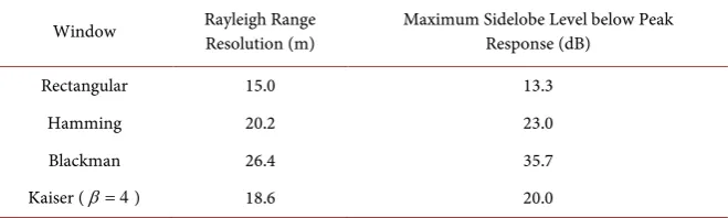
To achieve various compromises between Rayleigh range resolution [2] and peak sidelobe levels [14], the radar can use the CT rectangular, Hamming, Blackman, and Kaiser windows, mathematically described by [15]

( )

(

)

,

R avg M

w t = Π_ t−τ T _ (71)

( )

{

0.54 0.46 cos 2π 1

(

)

(

)

}

(

)

,

H M avg avg M

w t = + _ T t−τ _ Π_ t−τ T _ (72)

( )

{

(

)

(

)

(

)

(

)

}

(

)

0.42 0.5 cos 2π 1

0.08 cos 2π 2 ,

B M avg

M avg avg M

w t T t

T t t T

τ

τ τ

 

= + _ − _

   

+ _ − _ Π_ − _ (73)

(13)

[image:13.595.207.540.90.303.2]

Table 1. Parameters of simulated radar system.

Parameter Value

B 10 MHz

p

τ _{100 μs}

min

R 19.5 km

max

R 25.5 km

2

min Rmin c

τ = 130 μs

2

max Rmax c

τ = _{170 μs}

( ) 2

avg min max

τ =τ +τ 150 μs

( min)

(

avg min

)

p

f R =Bτ −τ τ 2 MHz

( max)

(

avg max

)

p

f R =Bτ −τ τ −2 MHz

M max min p

T =τ −τ +τ 140 μs

M M p

B =BT τ 14 MHz

( )

(

_{( )}

)

(

)

2

0

0 1 2

,

avg M

K avg M

I t T

w t t T

I

β τ

τ β

 ₋_ ₋ _ 

 _ _ 

 _{ } _

= Π_ − _ (74)

respectively. In Equation (74) I0 is the zeroth-order modified Bessel function of the first kind with shaping parameter β≥0. We choose

4

β =

₍₇₅₎

[image:13.595.210.540.499.705.2]

to specify a Kaiser window having a temporally broader characteristic than the Hamming and Blackman windows, as shown in Figure 4.

Table 2 shows the key performance characteristics corresponding to these four windows, assuming the returned pulse is temporally centered in each win-dow.

(14)

[image:14.595.209.539.91.190.2]

Table 2. Characteristics of available windows.

Window Rayleigh Range _{Resolution (m)} Maximum Sidelobe Level below Peak _{Response (dB)}

Rectangular 15.0 13.3

Hamming 20.2 23.0

Blackman 26.4 35.7

Kaiser (β=4) 18.6 20.0

For convenience of simulation, we set

N

y to 1 V2/Hz. We pass complex

white, Gaussian noise with independent, equal-variance real and imaginary parts through a fifth-order Butterworth lowpass filter with bandwidth By 2 and then spectrally translate the output noise by fy− fRF to obtain complex noise with a PSD closely approximating Equation (41). For each considered case, 10,000 Monte-Carlo runs produce the data used to simulate the PDFs (through histograms) and the autocorrelation functions (through sample averages). We simulate two types of BLGN having practical significance.

4.1. Case 1: Wideband Noise

For this case we set

,

y RF

f = f (76)

and we choose

(

)

20 MHz 2 18 MHz

y M max

B = >B − f R =

(77) to guarantee the BLGN’s PSD always fully fills the complex stretch processor’s “passband,” i.e., the interval _f R

(

_max

) (

,f R_min

)

_. This noise could represent internal receiver thermal noise or external broadband-noise jamming. Using Equation (63) and Equation (64), we determine that the BLGN corrupts the complex stretch processor’s output from fa= −2 MHz to fb=2 MHz (i.e., all output frequencies of interest to this complex stretch processor). Thus, we will only consider values of f1 and f2 on

[

−2 MHz, 2 MHz

]

. Equation (65) and Equation (66) then respectively give

(

1, 2

)

max

(

1, 2

)

7 MHz l

f f f = f f − (78)

and

(

1, 2

)

min

(

1, 2

)

7 MHz. u

f f f = f f + (79)

Substituting Equation (78) and Equation (79) into Equation (68) and Equa-tion (69) respectively gives

(

1, 2

) (

1 2

)

2 c

f f f = f + f (80) and

(

1, 2

)

14 MHz 1 2 .

eq

B f f = − f − f

(81)

(15)

( )

CM

Y f being WSS. By substituting Equation (80) and Equation (81) into Equa-

tion (70), we can approximate the autocorrelation function as

(

)

(

)

( )

(

)

[ ] [ ]

( )( )

(

)

( )( )

(

)

(

)(

)

(

)

(

)

{

}

(

)

4

1 2

2 2 6

1 2

2π 1.5 10

11 6

1 2 1 2

π 1960 π 14 10

2π 15 14 *

6 11 4

1 2 1 2

1 2

, 2 10 14 10 e

e e e

sinc 14 10 10 1.4 10

. CM

W W

CM

j f f Y

N N

j n m j n m f f

j n m

p p

n N m N

Y

R f f f f

W n W m

f f f f n m

R f f

−

− − ×

−

− − + − ×

−

=− =−

− −

≈ × × − −

×

 

× × − − _ − − − × _

= −

∑ ∑

₍₈₂₎

As expected, Equation (82) depends on only f1−f2, so the output noise is WSS for this case, regardless of the specific window employed.

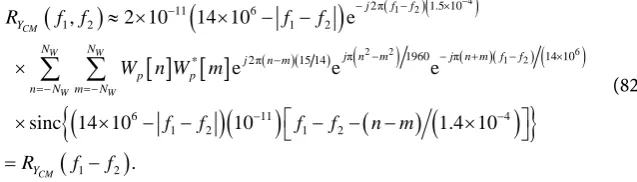
4.1.1. Case 1a: Rectangular Window

By substituting Equation (71) into Equation (28), we obtain

[ ]

1, 0 0, otherwise p

n

W n =  =

 (83)

as the exact Fourier coefficients necessary to evaluate Equation (82). After sig-nificant simplification we obtain

(

)

(

)

( )

(

)

(

)

(

)

4

1 2

2π 1.5 10

11 6

1 2 1 2

6 11

1 2 1 2

2 10 14 10 e

sinc 14 10 10

CM

j f f Y

R f f f f

f f f f

−

− − ×

−

− ≈ × × − −

 

× _ × − − − _

(84)

as the final expression for the output’s theoretical autocorrelation function. In agreement with [3] [4], for any frequency considered by the complex stretch processor, the output noise will have a variance of

( )

2

(

1, 1

)

2 4 2 2

0 2 2.8 10 V Hz .

CM

y p eq y p M

Y y M

N B f f N B

R N T

B B

τ τ ₋

≈ = = = × ₍₈₅₎

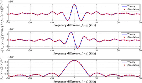
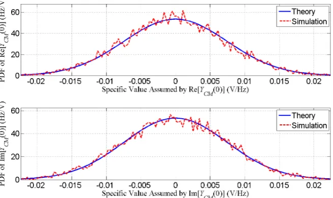
[image:15.595.215.534.109.200.2]

Figure 5 shows overlays of the theoretical and numerically approximated

[image:15.595.208.541.504.701.2]

(16)

DOI: 10.4236/jsip.2018.91003 51 Journal of Signal and Information Processing PDFs of the real and imaginary components of the complex stretch processor’s output at f1− f2=0. The theoretical PDFs are Gaussian with mean zero and variance _{0.5 2.8 10 V}

(

_× −4 2 _Hz2

)

₌_{1.4 10 V}_× −4 2 _Hz2 (since we expect the real and imaginary components to each have half the total noise variance). Clearly, the simulated output’s real and imaginary components both closely follow a Gaussian characteristic having the theoretically predicted mean and variance. The numerically approximated correlation coefficient for the simulated output’s real and imaginary components is −0.00073. Since this value is practically zero, the real and imaginary components are practically uncorrelated. Since the real and imaginary components are also Gaussian, they are practically independent, as previously stated.

Figure 6 shows excellent agreement between the theoretical and simulated autocorrelation functions. We conventionally consider output-noise compo-nents separated in frequency by a minimum of about 8.62 kHz (the 3-dB width of the main lobe of the autocorrelation function’s magnitude) to be practically uncorrelated. The 8.62-kHz frequency difference maps to a slant-range separa-tion of 12.93 m which is below this radar’s Rayleigh range resolusepara-tion of 15 m (10 kHz). Thus, if the radar samples the stretch processor’s output every 15 m (10 kHz), the BLGN-related components should be practically uncorrelated from one range sample to the next.

The complex correlation coefficient [16]

(

)

(

)

( )

(

)

( )

(

)

(

)

( )

{

}

(

)

( )

(

)

( )

(

)

( )

(

)

(

)

(

)

*

, cov

var var

,

, ,

CM

CM CM

CM CM CM CM

CM CM

Y

Y Y

f f f

Y f f Y f

Y f f Y f

E Y f f E Y f f Y f E Y f

Y f f Y f

E Y f f Y f

Y f f Y f

R f f f

R f f f f R f f

ρ + ∆

 + ∆ 

 

 

+ ∆

 

   

 + ∆ − _ + ∆ _  − _ _

   

=

+ ∆

   

   

 + ∆ 

 

=

+ ∆

   

   

+ ∆ =

+ ∆ + ∆



(86)

quantitatively characterizes the correlation between samples of YCM

( )

f at fre-quencies f + ∆f and f . Since YCM

( )

f is WSS for this case,

(

)

( )

, .

0

0 0

CM CM

CM

CM CM

Y Y

Y

Y Y

R f R f

f f f f

R

R R

ρ + ∆ = ∆ = ∆ =ρ ∆ ₍₈₇₎

We evaluate Equation (84) at ∆ =f 10 kHz and f =0 and substitute the re-sults into Equation (87) to obtain

(

10 kHz

)

(

10 kHz

_{( )}

)

0.2160 0.0000. 0

CM

Y

R

j R

ρ = ≈ + ₍₈₈₎

[image:16.595.226.539.382.551.2]

(17)

[image:17.595.73.540.75.349.2]

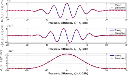
Figure 6. Theoretical and simulated autocorrelation functions for Case 1a.

4.1.2. Case 1b: Hamming Window

[ ]

( )

2π 15 14

0.23e , 1

0.54, 0

0.23e , 1

0, otherwise

j

p _j

n n

W n

n

−

 _{= −}



= 

= 

= 

 

(89)

as the exact Fourier coefficients necessary to evaluate Equation (82) in closed form. After significant simplification we obtain

(

)

(

)

( )

(

)

(

)

(

)

{

}

{

(

)

(

)

(

)(

)

{

(

)

4

1 2

2π 1.5 10

11 6

1 2 1 2

2 2 6

1 2

6 11

1 2 1 2

6

1 2

2 10 14 10 e

0.54 2 0.23 cos 2π 14 10

sinc 14 10 10

2 0.54 0.23 cos π 14 10 π 1960

CM

j f f Y

R f f f f

f f

f f f f

f f

−

− − ×

−

− ≈ × × − −

 

× + _ − × _

 

× _ × − − − _

 

+ _ − × − _

(

)

(

)

(

)

(

)

(

)

}

(

)

{

(

)

(

)

(

)

(

)

}

6 11 4

1 2 1 2

6

1 2

6 11 4

1 2 1 2

2 6 11 4

1 2 1 2

6 11 4

1 2 1 2

sinc 14 10 10 1 1.4 10

cos π 14 10 π 1960

sinc 14 10 10 1 1.4 10

0.23 sinc 14 10 10 2 1.4 10

sinc 14 10 10 2 1.4 10

f f f f

f f

f f f f

− −

 

× _ × − − − − × _

 

+ _ − × + _

 

× _ × − − − + × _

 

+ _ × − − − − × _

 

+ _ × − − − + × _

(18)

DOI: 10.4236/jsip.2018.91003 53 Journal of Signal and Information Processing as the final closed-form expression for the output’s theoretical autocorrelation function. For any frequency considered by the complex stretch processor, the output noise will have a variance of about

( )

₀ _{1.113 10}4_V2 _{Hz .}2 CM

Y

R ≈ × − (91)

Figure 7 shows overlays of the theoretical and numerically approximated PDFs of the real and imaginary components of the complex stretch processor’s output at f1– f2=0. The theoretical PDFs are Gaussian with mean zero and variance _{0.5 1.113 10}

(

_× –4_V2 _Hz2

)

₌_{5.56 10}_× −5_V2 _Hz2. Clearly, the simulated output’s real and imaginary components both closely follow a Gaussian charac-teristic having the theoretically predicted mean and variance. The numerically approximated correlation coefficient for the simulated output’s real and imagi-nary components is 0.0047, indicating the two Gaussian components are practi-cally independent.

Figure 8 shows excellent agreement between the theoretical and simulated autocorrelation functions. Using the previously stated convention, we consider output noise components separated in frequency by a minimum of about 17.3 kHz to be practically uncorrelated. This frequency difference maps to a slant- range separation of 25.9 m which exceeds this radar’s Rayleigh range resolution of 20.2 m by about 28%. If the radar samples the stretch processor’s output every 20.2 m (13.47 kHz), the BLGN-related components in any two adjacent range samples will have a complex correlation coefficient of

(

13.467 kHz

)

RY_CM

(

13.467 kHz

)

RY_CM

( )

0 0.1685 j0.0209.

ρ

= ≈ − (92)

Since ρ

(

13.467 kHz

)

is approximately 0.1698, the two samples of Y_CM

( )

f

[image:18.595.212.540.508.703.2]

are only slightly correlated despite the radar’s range-sampling interval being somewhat less in extent than the conventionally defined range-decorrelation in-terval.

(19)

[image:19.595.95.540.78.338.2]

Figure 8. Theoretical and simulated autocorrelation functions for Case 1b.

4.1.3. Case 1c: Blackman Window

[ ]

( )

2π 15 7

2π 15 14

2π 15 7

0.04e , 2

0.25e , 1

0.42, 0

0.25e , 1

0.04e , 2

0, otherwise

j

p j

j

n n n

W n

n n

−

 = −



= − 

= 

= 

= 

 ₌

 

(93)

as the exact Fourier coefficients necessary to evaluate Equation (82) in closed form. Note: For NW =2, the double summation in Equation (82) produces

(

)

2

2N_W+1 =25 terms; even after significant simplification, the closed-form expression for the theoretical autocorrelation function is relatively unwieldy, so we omit it. For any frequency considered by the complex stretch processor, the complex output noise will have a variance of about

( )

5 2 2

0 8.529 10 V Hz . CM

Y

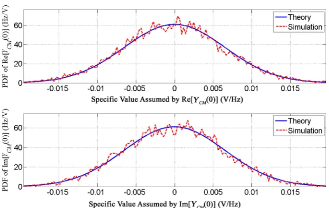
R ≈ × − (94) Figure 9 shows overlays of the theoretical PDFs and the numerically approx-imated PDFs of the real and imaginary components of the simulated complex stretch processor’s output at f1− f2=0. The theoretical PDFs are Gaussian with mean zero and variance

(

–5 2 2

)

5 2 2

[image:19.595.300.445.404.486.2]

(20)

[image:20.595.213.535.66.270.2]

Figure 9. Theoretical and simulated PDFs for Case 1c.

[image:20.595.86.540.438.702.2]

components are practically independent.

Figure 10 shows excellent agreement between the theoretical and simulated autocorrelation functions. Using the previously specified convention, we con-sider output noise components separated in frequency by a minimum of about 22.3 kHz to be practically uncorrelated. This frequency difference maps to a slant-range separation of 33.5 m which exceeds this radar’s Rayleigh range reso-lution of 26.4 m by about 27%. If the radar samples the stretch processor’s out-put every 26.4 m (17.6 kHz), the BLGN-related components in any two adjacent