Control and implementation of a transfemoral prosthesis for walking at different speeds

Control and Implementation of

a transfemoral prosthesis for

walking at different speeds

F. (Feite) Klijnstra

MSc Report

Committee:

Prof. dr. ir. S. Stramigioli

Dr. R. Carloni

R. Unal, MSc

Dr.ir. R.G.K.M. Aarts

Oktober 2012

Report nr. 028RAM2012

Robotics and Mechatronics

EE-Math-CS

University of Twente

P.O. Box 217

Contents

1 Introduction 2

2 Paper 1:

Modeling of a Fully-Passive Transfemoral Prosthesis

Prototype 3

3 Paper 2:

Control and implementation of an energy efficient

transfemoral prosthesis for walking at different speeds 9

4 Conclusion 15

Appendices 16

A Controller code 16

B Electrical diagrams 18

1

Introduction

In this work two papers will be presented. The first paper is about modeling a transfemoral prosthesis to create more insight in the energetic behaviour of the prosthesis. The model is obtained in previous work and improved to be able to create this insight. The topic will be further introduced in the paper itself.

The second paper describes the design and realisation of a new prototype of the transfemoral prosthesis which is capable to adapt to different walking speeds. An actuator with control system is designed to achieve this adaptive behaviour and first test show the system is working.

Modeling of a Fully-Passive Transfemoral Prosthesis Prototype

F. Klijnstra, B. Burkink, R. Unal, S. Stramigioli, H.F.J.M. Koopman and R. Carloni

Abstract— In this paper we present the modeling of a fully-passive transfemoral prosthesis prototype, which has been designed and realized for normal walking. The model has been implemented in a simulation environment so to analyze the behavior of the prosthetic leg in different walking conditions and so to enhance the mechanics of the system. The accuracy of the model has been validated in experimental tests, supported by the help of an amputee.

I. INTRODUCTION

A transfemoral prosthesis is an assistive device, which artificially replaces the lower limb after an amputation due to a trauma or a disease. The challenging part in designing and realizing such a device is in reducing the use of metabolic energy consumption while restoring the gait pattern of the amputee with a light-weighted and intuitive system.

In our previous work, we designed and realized a fully-passive transfemoral prosthesis prototype for normal walk-ing, which provides 76% of the required energy for the ankle push-off generation [1], [2]. The conceptual design is based on the analysis of the energetics of walking of the natural human gait with the final goal of having an energy efficient device [3], [4]. This is done by including three elastic elements, which realize an energetic coupling between the knee and the ankle joints. More precisely, three elastic elements are engaged in the different phases of the stride and they mimic the muscles synergies found in the healthy human gait. The overall system is fully-passive and the only supplied energy comes from the hip joint of the transfemoral user.

At the current stage of our research, a detailed dynamic model is necessary to investigate how the transfemoral pros-thesis prototype is performing in different walking conditions and with different amputees biomechanical characteristics. The model will be used for the analysis of the transfemoral prototype to look for further improvements and eventually realisations. For this reason, we realized a port-based model in a simulation environment, which founds its basis on screw theory, and we validated it through experimental tests realized with the help of an amputee.

The creation of a dynamic model to generate gait patterns poses challenges such as the rate of complexity and the adaptability to design changes. In [5] a model of human body

This work has been funded by the Dutch Technology Foundation STW as part of the project REFLEX-LEG under the grant no. 08003.

F. Klijnstra, B. Burkink, R. Unal, S. Stramigioli and R. Carloni are with the Faculty of Electrical Engineering, Mathematics and Computer Science, University of Twente, The Netherlands; R. Unal and H.F.J.M. Koopman are with the Faculty of Biomechanical Engineering, University of Twente, The

Netherlands. Emails: {f.klijnstra, b.burkink}@student.utwente.nl, {r.unal,

s.stramigioli, h.f.j.m.koopman, r.carloni}@utwente.nl

(a) Prototype

Shank

Foot

Telescopic Springs Ankle

Knee

Ankle Springs Linkage

Slider

(b) CAD drawing

Fig. 1: Mechanical realisation of the transfemoral prototype.

dynamics is shown using a mechanical multi body systems approach. A downside of this approach is the long derivation of the dynamic equations, which can be error prone and changes in the design cause long implementation time in the model.The same strategy of mathematical modeling has been used in [6] and [7]. The models built are all made for the purpose of obtaining gait patterns.

The remainder of the paper is organized as follows. Section II presents the working principle of the transfemoral prosthesis prototype. The complete model of the system is presented in Section III and validated in Section IV through experimental tests. Finally, conclusions are drawn in Section V.

II. WORKING PRINCIPLE OF THE TRANSFEMORAL PROSTHESIS

The transfermoral prototype is shown in Fig. 1, in which both a picture of the realized system and a detailed CAD drawing are reported.

The transfemoral prosthesis is a fully-passive system, which has been designed and realized to mimic the human gait energetics [2].

Fig. 2 shows the power flow at the knee (top) and ankle (bottom) joints in a healthy human during a normal gait [8]. In the figure, it is possible to identify three instants, i.e. heel strike, push-off and toe-off, and three main phases:

• Stance: the knee absorbs a certain amount of energy

-1 -0.8 -0.6 -0.4 -0.20 0.2 0.4 0.6 0.8

0 20 40 60 80 100

-0.5 0 0.5 1 1.5 2 2.5 3 3.5

0 20 40 60 80 100

%of stride

Ankle po wer [W/kg] Knee po wer [W/kg]

A1 A2

A3 G

Heel-Strike Push-Off Toe-Off Heel-Strike

Ankle po wer [W/kg] Knee po wer [W/kg]

A1 A2

A3 G

Stance Pre-swing Swing

normal

Fig. 2: Power flow in the normal human gait as reported by Winter in [8].

The areasA1,2,3indicate the energy absorption, whereasGindicates the

energy generation. The cycle is divided into three phases (stance, pre-swing and swing) with three main instants (heel-strike, push-off and toe-off).

• Pre-swing: the knee starts absorbing energy, represented byA1in the figure, while the ankle generates the main part of the gait energy for the push-off, represented by

G, which is about the80%of the overall generation.

• Swing: the knee absorbs energy, represented by A2 in

the figure, during the late swing phase, while the energy in the ankle joint is negligible.

These energetic phases show that there is almost a complete balance between the generated and the absorbed energy, since the energy for push-off generation (G) is almost the same as the total energy absorbed in the three intervalsA1,2,3.

In its working principle, the transfemoral prosthesis ab-sorbs energy during stance, swing phase and heel strike and releases energy during ankle push-off. This has been realized by using three storage elements depicted in 3 and explained hereafter, i.e.,

• The coupling elastic element (i.e., a telescopic spring)

C2 couples the upper and lower leg. It is responsible

for the absorption and transfer of A2 and for a part of the absorptionA3 during stance phase.

• The ankle elastic element C3 connects the foot and

lower leg and is responsible for the main part of the absorptionA3.

• The linkage mechanismCLcouples the knee and ankle joints kinematically and is responsible for the transfer of a part of A1 to the ankle push-off generation (G).

III. MODEL

In this Section we present the model of the transfemoral prosthesis. First, we give a short overview of the notations and of the mathematical framework and second, each part of the device is discussed in details.

Fig. 3: Conceptual design of the proposed mechanism (given separately

for better interpretation) - The design presents three elastic elements:C2

between the foot and the upper leg,C3between the foot and the lower leg

(left), a linkage systemCLbetween the knee and ankle joints (right).

A. Bond graphs and Screw Theory

The dynamic model of the system is developed using screw theory and the port-based approach that makes use of bond-graphs as a graphical representation. The port-based approach and the bond-graphs are suitable for multi-domain dynamic modeling and screw theory provides the mathematics that are needed to describe the kinematics and dynamics of the system. The combination of these methods provides a good tool to model a complex dynamic system such as the transfemoral prosthetic prototype. The bond-graph representation is used to implement the Newton-Euler equations of rigid bodies in a principal frameΨ0without the need of writing the complete dynamic equation of motion. The construction of the dynamic model has been realized in the simulation environment 20-Sim [9]. More information on the mathematical framework can be found in [10].

B. Overall Kinematics

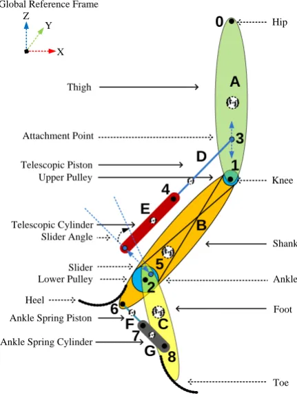
A complete overview of all the joints and bodies of the transfemoral prosthesis are shown in Fig. 4.

Every joint is described in its coordinate frame. The joints

0,1,2,3,6,8are rotational joints and can rotate freely around their localy direction. The joints 4 and7 are translational joints and can translate freely along their local z direction, so to realize the telescopic and ankle springs. The joint 5

can both translate along its local z direction and can rotate around its local y direction, so to realize the slider action. All joints are summarized in Table I.

TABLE I: Joint representation and degrees of freedom (DOFs) with respect to local reference frames.

Joint in the physical System Joint number Local DOFs

Hip 0 X, Z and Ry

Knee 1 Ry

Ankle 2 Ry

Upper Attachment Point 3 Ry

Telescopic Spring 4 Z

Slider 5 Ry and Z

Heel Attachment Point 6 Ry

Ankle spring 7 Ry

Thigh

Foot Shank Telescopic Piston

Telescopic Cylinder

Ankle Spring Cylinder Ankle Spring Piston Slider Ankle Knee Hip Lower Pulley Upper Pulley

A

B

C

D

E

0

1

2

3

4

5

F

G

6

7

8

Global Reference Frame

Heel

Toe

Fig. 4: Schematic overview of the transfemoral prosthesis, where bodies are represented by letters and joints by numbers.

C. Telescopic and Ankle Springs

The location of the telescopic spring is joint4. The tele-scopic spring has a progressive behaviour [1]. In particular, the force exerted by the telescopic spring depends on the spring statexand on the elastic constants of the three springs that are progressively engaged, i.e.,

Ftelescopic=

      

k1 (x₋x0) 0< x < s1 (k1+k2) (x₋x0) s1< x < s2 (k1+k2+k3) (x₋x0) x > s2 k0 (x₋x0) x <0

wherex0 is the zero length of the spring andki the elastic constants.

The ankle spring is a linear spring with kf oot as elastic constant. The force exerted by this spring is given by

Fankle=kf oot·(x−x0) x >0

wherex0 is the zero length of the spring.

D. Linkage

The linkage is located between the knee and ankle joints, as shown in Fig. 4. This element can be modeled as a conditional spring since it is not continuously active. If the spring is active it will be acting between the ankle and knee, otherwise there will be no physical connection.

The connection is activated just after stance, at a certain ankle angle, until there is no force on it anymore. Then the connection is disengaged and the ankle and knee are not coupled any more.

Telescopic Cylinder Foot Slider Spindle _M c c d d M c c d d Front Position Back Position Trajectory

(a) Foot of the prototype with the slider and telescopic cylin-der.

(b) Slider Schematic.

Fig. 5: Slider

E. Slider

The slider can move freely along the localz direction of the joint5, as shown in Fig. 4. In Fig. 5b, the mass represents the telescopic cylinder in Fig. 5a.

The following relations hold for the inner and outer bounds for the front and back position of the slider.

front=

outer bound always valid

inner bound φankle< φreleaseankle

back=

outer bound always valid

inner bound telescope is pulling

where φreleaseankle = 6

◦_{. The outer bounds resemble the}

front and back end position of the slider since it can not move any further in the physical system [1]. The inner bound on the back of the slider models the notch at the back of the slider.

F. Ground Reaction Forces

The implementation of the ground reaction forces is based on the Hunt-Crossley model for ground interaction described in [11]. The Hunt-Crossley contact model is used to calculate the normal force, which is exerted by the ground, and the friction force, which acts parallel to the ground.

In the dynamic simulation of the model, the contact point is calculated as the closed contact from a circle (e.g., the heel profile) with respect to another point (e.g., the ground), to create the necessary roll-over, as explained in [12].

G. Model’s Inputs

The inputs of the model are only the forces applied by the amputee on the prosthesis. Therefore, in order to validate the dynamics model, the angle of the hip measured during the experimental tests are used. Furthermore, the force of the sound leg is put in the model by applying the ground reaction forces in the x and z direction of the hip. These forces are used because the forces on the prosthesis are not directly measured. The rest of the system behaves according to the dynamical model.

H. Model Overview

Fig. 6: Complete overview of the implemented dynamic model.

controlled by a PD-controller which controls the torque on the hip joint.

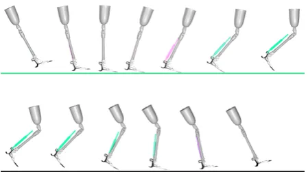
Fig. 7 shows an example of gait pattern for normal walking in a simulation of the dynamic model.

IV. VALIDATION OF THE MODEL

In this Section, we validate the dynamic model by using real inputs as taken from experimental tests done with the help of an amputee.

A. Experimental Test Set-up

The experimental test set-up consists of a treadmill with speed control. The transfemoral prosthesis is equipped with markers for tracking the movements with a motion tracking system. Force plates are placed under the track of the tread-mill to measure ground reaction forces. If these forces are applied to the model then the resulting power and torque of the joints can be generated. For the simulation it is necessary to measure the hip angle and ground reaction forces from the sound leg as these are used as an input on the model.

Figure 8 shows the transfemoral amputee with his own socket and the transfemoral prosthesis prototype. A full gait pattern for normal walking is shown in Fig. 9.

Fig. 7: Human Gait overview of the simulation. The colors resemble the loading and unloading of the telescopic spring. Green is unloaded and purple is loaded.

Fig. 8: The transfemoral amputee is wearing the prosthesis with his own socket.

B. Validation of the Model

In Fig. 10 the angles of the hip, knee and ankle are shown as derived from the simulation of the model (continuos line), measured data from the amputee (dashed line) and the data from a healthy subject as presented in [8] (dashed-dotted line). From the plots, it can be seen that the angles of the model simulation are nicely following the angles of the measured data from the functional tests.

The difference of the knee angle during stance is due to the fact that the prosthesis does not flex during stance but is constrained in hyperextension.

Fig. 9: Gait cycle of the amputee -30 -20 -10 0 10 20 30

0 20 40 60 80 100

hip angle ( ◦) -20 0 20 40 60 80

0 20 40 60 80 100

knee angle ( ◦) -30 -20 -10 0 10 20

0 20 40 60 80 100

ankle

angle

(

◦)

%of stride

Winter Amputee Simulation

Fig. 10: The hip, knee and ankle angles during normal walking for both the amputee and the simulated model.

in positive direction. Then when the slider is in the front position and it is still pushing, the ankle angle is forced to move in negative direction. If the knee angle then decreases, the telescope starts pulling and the ankle is forced again to move in positive direction. This process is sensitive to gait timing and, due to small timing differences between the simulation and the real test, the model simulation and the experimental tests differ.

C. Discussion

In this section the model will be compared with the data of a healhty human to analyse the working of the prosthesis which was one of the goals of the model. The joint torques of the knee and ankle are shown in Fig. 11. In this plots, only the data from the model simulation are shown because the joint torques are not directly measured in the experiments with the amputee.

The positive knee torque during stance is due to the hyperextension. Around60%of stride, a positive knee torque is present and it is due to the telescope spring that is pushing and, therefore, causing a higher hip angle input. In the ankle torque, the roll-over torque builts up later in the gait because the ankle springs only start loading from 0◦.

-20 -10 0 10 20 30 40

0 20 40 60 80 100

-40 0 40 80 120 160 200

0 20 40 60 80 100

%of stride

Ankle torque [Nm] Knee torque [Nm]

Fig. 11: The knee and ankle torques in the model simulation.

-150 -120 -90 -60 -30 0 30 60

0 20 40 60 80 100

-300 -200 -100 0 100 200 300 400

0 20 40 60 80 100

%of stride

Ankle po wer [W] Knee po wer [W] Simulation Winter

Fig. 12: The knee and ankle power in the model simulation. The absorption and generation areas are present in the expected phases.

roll-over energy is stored in a smaller range. The early toe-off, visible in the plot, is due to the fact that the energy is released in a smaller time range then in an healthy human.

The dynamic model of the transfemoral prototype is overall working correctly and it has been validated through experimental tests. The model can be used to produce the torque and power plots, which can show the performance of the prosthesis and therefore can be used to improve the mechanical design of the prototype. Measuring these values directly on the prototype is very difficult so a model to obtain the values is the best solution.

The results of the experimental tests show that the proto-type is working as expected. The hip angle input is larger in comparison with the reference data of Winter discussed in sec. II, the hip provides15◦more in the stance phase. This is most likely the result of the fact that the amputee wants to be sure that the knee goes in hyperextension. This can be solved if the prosthesis is able to store different energy amounts in the telescope spring. In this way it can ensured the knee will go in hyperextension and the amputee can reduce the extra hip input.

V. CONCLUSIONS

In this work it is shown that the modeling of the prosthesis can be done as described with screw theory and bond graph representation. The complex model obtained shows the pros-thesis is working as expected. The torque and power plots are used to create more insight in the energetic behaviour of the prosthesis. These torque and power plots show similarities with the natural torque and power profiles which was one of the goals of the prosthesis. The insight obtained by the model will be used to improve the prosthesis in future prototypes.

VI. ACKNOWLEDGMENTS

The authors are thankful to the anonymous amputee for the willingness of helping in the project along the validation of the model.

REFERENCES

[1] S. Behrens, R. Unal, R. Carloni, E. Hekman, S. Stramigioli, and H. Koopman, “Design of a fully-passive transfemoral prosthesis

pro-totype,” inProceedings of the IEEE/EMBS International Conference

of Engineering in Medicine and Biology Society, 2011.

[2] R. Unal, R. Carloni, S. Behrens, E. Hekman, S. Stramigioli, and H. Koopman, “Towards a fully passive transfemoral prosthesis for

normal walking,” insubmitted to the IEEE International Conference

on Robotics and Automation, 2012.

[3] R. Unal, S. Behrens, R. Carloni, E. Hekman, S. Stramigioli, and H. Koopman, “Prototype design and realization of an innovative

energy efficient transfemoral prosthesis,” in Proceedings of the

IEEE/EMBS International Conference on Biomedical Robotics and Biomechatronics, 2010.

[4] R. Unal, R. Carloni, E. Hekman, S. Stramigioli, and H. Koopman, “Conceptual design of an energy efficient transfemoral prosthesis,” in

Proceedings of the IEEE/RSJ International Conference on Intelligent Robots and Systems, 2010.

[5] M. Stelzer and O. Von Stryk, “Efficient forward dynamics

simu-lation and optimization of human body dynamics,” ZAMM-Journal

of Applied Mathematics and Mechanics/Zeitschrift fr Angewandte Mathematik und Mechanik, vol. 86, no. 10, pp. 828–840, 2006. [6] V. Berbyuk and B. Lytvyn, “Mathematical modeling of human walking

on the basis of optimization of controlled processes in biodynamical

systems,”Journal of Mathematical Sciences, vol. 104, no. 5, pp. 1575–

1586, 2001.

[7] V. Berbyuk, G. Grasyuk, and N. Nishchenko, “Mathematical modeling

of the dynamics of the human gait in the saggital plane,”Journal of

Mathematical Sciences, vol. 96, no. 2, pp. 3047–3056, 1999.

[8] D. Winter,Biomechanics and motor control of human gait: normal,

elderly and pathological. University of Waterloo Press, 1991.

[9] 20-Sim. Controllab products. [Online]. Available:

http://www.20sim.com

[10] V. Duindam, A. Macchelli, S. Stramigioli, and H. Bruyninckx,

Model-ing and Control of Complex Physical Systems - The Port-Hamiltonian Approach. Springer, 2009.

[11] S. Stramigioli and V. Duindam, “Port based modeling of spatial

visco-elastic contacts,” European Journal of Control, vol. 10, no. 5, pp.

505–514, 2004.

Control and implementation of an energy efficient transfemoral

prosthesis for walking at different speeds

F. Klijnstra, R. Unal, S.M. Behrens, S. Stramigioli, H.F.J.M. Koopman and R. Carloni

Abstract— In this work the control and implementation of energy efficient prosthesis for walking at different speeds will be shown. The prototype is based on previous work and makes use of energy flow during seen in healthy human gait. An actuator is designed to change the configuration of the prosthesis to adapt for different speeds. First test show that the prototype is working but more tests have to be performed to show the energy efficiency of the prosthesis.

I. INTRODUCTION

The use of transfemoral conventional passive prosthe-ses for walking requires 65% more metabolic energy then healthy people, due to the absence of muscles and tendons [1], [2], [3]. When walking on varying speeds this energy consumption will be even higher, due to the invariable dynamics of these prostheses [4], [5].

Currently three categories of prostheses can be classi-fied; passive, controlled and powered. Passive prostheses are designed to exploit the dynamics of walking to create the gait cycle of the prosthesis. These type of prostheses are mechanically efficient but the absence of ankle push-off and the invariable dynamics reduce the efficiency of walking drastically [6]. Controlled prostheses can change their dynamics with actuators to adapt for different walking conditions but do not inject power in the gait cycle. It is shown that these type of prosthesis reduce the oxygen consumption during walking at varying speeds [4], [5]. Powered prostheses are able to inject energy in the gait cycle with their actuators to reduce the need of extra metabolic energy but require a external power source to get the energy from [7].

To reduce the use of metabolic energy a prosthesis should be energy efficient. This can be done by studying power flow in healthy human gait as has been done in [8]. In this study the work of Winter [9] is used to see how the energy is used in healthy subjects and try to mimic this energy flow. Energy is stored during certain parts of the gait cycle and released during other parts, especially the push off. With the use of this study a new concept of a prosthesis is come up with which uses springs to store energy and different mechanisms to distribute it [10]. This prosthesis should be able to perform this task also at varying walking speeds to reduce the extra metabolic energy consumption during this changing conditions.

In this work a new prototype will be presented which is able to change the configuration to store different amounts of energy that are imposed by the varying walking speeds. The actuator used to change the configuration will use minimal

-2.5 -2 -1.5 -1 -0.50 0.5 1 1.5

0 20 40 60 80 100

-1 0 1 2 3 4 5

0 20 40 60 80 100

%of stride

Ankle po wer [W/kg] Knee po wer [W/kg] A1 A2

A3 G

Heel-Strike Push-Off Toe-Off Heel-Strike

Ankle po wer [W/kg] Knee po wer [W/kg] A1 A2

A3 G

Stance Pre-swing Swing

slow normal fast

Fig. 1: Power flow during normal human gait with different speeds: slow (3.6km/h), normal (4.8km/h) and fast (6.3km/h). Data from Winter [9]

actuation to reduce the energy consumption as much as possible.

II. HUMAN GAIT

In this section the basic concepts of the prosthesis will be briefly explained. The prosthesis is based on the power flow of normal human gait[8]. In fig. 1 the power flow of normal human gait is visible. In this plot the power flow during the three phases of human gait can be seen:

• Stance: During first part of stance the knee absorbs the impact of heel strike by knee flexion and gives this energy back by extension. The ankle absorbs the rollover energy A3.

• Preswing: The ankle generates around 80% of the total energy generation during push-off. The knee starts absorbing energyA1.

• Swing: The knee starts absorbing energyA2during late

Energy (J/kg) A1 A2 A3 G ratio A/G

Slow 0.042 0.07 0.10 0.22 0.98

Normal 0.09 0.11 0.13 0.35 0.91

Fast 0.22 0.13 0.06 0.48 0.89

TABLE I: Energy levels of human gait with different speeds

the energy levels A1, A2, A3 and G can be found for the

three different speeds. The absorption of energy in the knee is clearly increasing when the walking speed increases but the absorbtion of energy in the ankle does not show such a relation. The generation part of the ankle however does again show the same increase.

III. CONCEPTUAL DESIGN

The conceptual design of the prosthesis shown in this work is based on the concept shown in [8]. The concept uses different springs to store the absorption parts of the power plots shown in the previous section and releashes the energy during push-off. In figure 2 the different spring elements are shown.

C1

C2

C3

x0

Fig. 2: Conceptual design of the prosthesis, the three elastic elements,C1,C2 andC3, and the slider are visible

This design process gives an energy efficient prosthesis but still lacks flexibility. This is because the amounts of energy that can be stored are fixed by the configuration and the elastic constants of the spring elements. As already shown in section II the energies are changing for different walking speeds. To be able to walk with different speeds the prosthesis should change the configuration in such a way that it stores the amount of energy according to the walking speed.

By changing the zero-length of the C2 spring, shown as

x0in fig. 2, the amount of energy stored during swing can be

changed. In the previous prototype changing the zero-length ofC2can be done manually but therefore not during walking.

To be able to walk dynamically with different speeds a system should be added to the prosthesis that can change this setting while the patient is walking.

The development of this system will be explained in the next sections.

A. Controller

In fig. 3 a schematic overview of the controller is shown. The different blocks of the controller will be explained hereafter. First the feedforward part of the controller, shown in the gray and white striped part, will be explained and after that the learning part of the controller, in the gray shaded part, will be shown. The mechanical part of the prosthesis is indicated as Walk MECH in the diagram with on the top the hip input of the human, on the bottom the measured knee angle and on the left side the input of the actuator.

The first block in the feed forward part in the diagram, denoted withTstr, uses the knee angle to find the stride time. This gives a measure for the walking speed and can therefor be used to know how much energy has to be stored in the springs. In fig. 4 it is shown how the stride is calculated from the knee angle. By looking at a certain knee angle and take the time between the next occurrence of this angle, with the same angular velocity, the stride time can be found.

-10 0 10 20 30 40 50 60 70 80

0 0.5 1 1.5 2 2.5

Knee angle ( cir c )

Stride time (s) Tstr

Fig. 4: Plot of the knee angle of 2 strides to show how the stridetime can be calculated

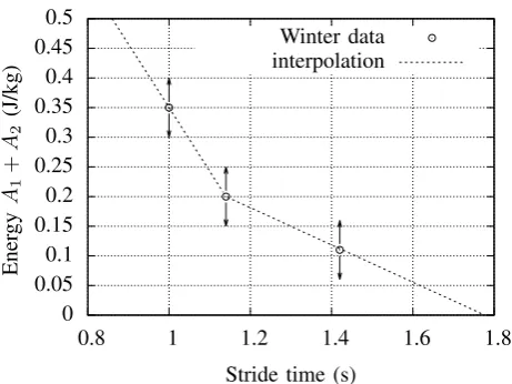
The next block, indicated with model, in the diagram estimates the amount of energy that needs to be stored in springC2 with the use of previous found stride time. Since

the amount of energy is related to the walking speed and therefore the stridetime, a relation between the stride time and energy amount A1+A2 is found. Winters data [9] of

the energy is plotted for slow, normal and fast in fig. 5 to find this relation. A simple double linear interpolation of the three points is also shown and the relation is shown in eq. 1, whereEA1+A2 is the energy ofA1+A2andtstris the stride

time. More smooth fits can be found with exponential and loglog relations but these require more complex calculations which undesirable when the energy levels are changed by the learning controller shown in the next section.

EA1+A2=

1.42₋1.07_·tstr tstr<1.14s

Knee Angle

Stride time Energy Setpoint Zero-length Knee speed on 0◦

Desired knee +

-Error on knee speed

Model x0=

q

2·E·w

k PD Prosthesis

Hip input Learning Controller Tstr -+ Actuator speed on 0◦

Feedforward d

dt

Walk MECH K

Fig. 3: Diagram of the learning controller

0 0.05 0.1 0.15 0.2 0.25 0.3 0.35 0.4 0.45 0.5

0.8 1 1.2 1.4 1.6 1.8

Stride time (s)

Ener gy A1 + A2 (J/kg) Winter data interpolation

Fig. 5: Relation between the stride time and energyA1+A2,

the arrows indicate the action of the learning controller

This relation then is used in the next block to find the right zero-length for spring C2. The relation between the stored

amount of energy and elongation of the spring is given by eq. 2, the value of the elongation for normal walking (xnormal) is substracted to get the setpoint, x0, for the actuator. k is

the stiffness ofC2andw is the weight of the amputee.

x0=

r

2_·EA1+A2·w

k −xnormal (2)

The generated setpoint will then be used by the PD controller to control the actuator to the right x0 as shown

in the last part of the feedforward system.

B. Learning controller

The method described in the previous sections is a feed-forward way to calculate the setpoint from the stridetime and has no feedback. The goal of the prothesis is to match the healthy human gait as close as possible so this should be ideal. But since there are clearly differences between the prosthesis and a normal human leg, it is desirable to have some feedback on the model between the stridetime and the stored amount of energy. Therefor a learning controller is

proposed in this subsection. This process is also shown in the diagram in fig. 3 as the gray shaded part.

The learning controller changes the model between the stridetime and energy according to an error. Ideally the knee will have zero angular velocity when it reaches hyperex-tension because then all the kinetic energy of the lower leg will be stored. This might not be desirable for the amputee because it imposes a risk that the knee will not reach hyperextension so a small velocity will be needed. If the amputee gives a bigger input this will result in a larger speed at hyperextension and this can be defined as an error when the desired speed is substracted. This error will be used to change the mapping as described hereafter.

The model will be changed by updating 2 energy points shown in fig. 5 where the current stridetime lies in between. The amount of change will also be depending on how close the current stridetime lies to the point. This will be implemented using Iterative Learning Control (ILC) and the general form of the algoritm is shown in eq. 3, whereui is a setpoint,ui−1 the previous setpoint, K the learning gain

andean error. More on ILC can be found in [11] and [12].

ui=ui−1+K·e (3)

The algorithm with the modifications as described before will look like eq. 4, where i is the current step, n is the point to be changed (can be slow, normal or fast),v0◦ is the velocity of the knee at 0◦ andvd 0◦ is the desired velocity at0◦. This example is for an energy point with a stride time less then the current stride time.

Ei,n=Ei−1,n+

_t

str,n−tstr

tstr,n+1−tstr,n

·K_·(v0◦−v_d0◦) (4)

From the new energy points the interpolated linear fit will be recalculated to get the new map from stride time to energy.

IV. REALISATION

designed to fit in the design of the proshesis and will be used to change the zero length as discussed in the previous section. In this section first the realisation the actuator will be discussed and then realisation of the control system also proposed in the previous section will be shown.

Fig. 6: Picture of the finished prosthesis

A. Actuator design

The design of the actuator is made with the idea of minimal actuation in mind to keep the prosthesis as energy efficient as possible. Therefore the actuator will be very light, compact and equipped with only a small motor to reduce the power consumption. The forces on the actuator on the other hand will be large because it will be in series with spring C2 and will therefore be subjected by high forces coming

from the human input. To keep the power consumption and the requirements of the motor low the zero-length will only changed during a small part of the gait cycle when the spring is unloaded. To keep the zero-length from changing during the loaded part of the gait, a non-backdrivable transmission is chosen. A DC-Gearmotor (Faulhaber, Germany), which is fitted with a 1:8 gearbox and an optical encoder, is chosen in combination with a trapezoidal spindle. The motor is coupled with the spindle via an oldham coupling to be sure there are no alignment problems and only the torque of the motor is transmitted to the spindle. A bush bearing provides the concentric alignment and handle the radial forces and bending moment. Slide bearings are used to handle the axial load and are chosen for their compactness and ability to handle the high axial forces applied on the actuator. In fig. 7 a section view of the actuator is shown with the different parts indicated.

B. Electrical system

To implement the controller as described in the conceptual design section, a system based on an arduino microprocessor

DC-Gearmotor

Trapezoidal spindle

Nut

Oldham coupling

Slide bearings

Bush bearing with encoder

Fig. 7: Section view of CAD drawing of the actuator, indicated are the important parts

is used. The optical encoder on the motor is used to measure the position of the actuator. To measure the knee angle, nec-essary for the controller, a magnetic encoder is used. These encoders provide contactless and high resolution (12bit) angle measurement and are light and compact. A second encoder is used to measure the ankle angle to compare the angles with those of a healthy human and the previous prototype. The Arduino Nano board is placed on a custom PCB to house the connectors and also a H-bridge to control the input to the motor. The data recorded on by the arduino can be sent to a computer via a serial port, this can either be done via an usb cable or wireless with a bluetooth or Xbee (Digi International, USA) module.

C. Controller

The controller is programmed on the arduino according to the diagram shown in fig. 3 found in sec. III. The differen blocks explained in that section are written in different functions which can be found in the appendices of this work.

V. RESULTS

In this section the results of the first trials will be shown. First the test setup is shown and some of its limitations mentioned.

A. Test setup

The prosthesis is first tested with healthy subjects to test whether the principle is working. This is done with healthy subjects to know for sure that when an amputee is willing to test the prosthesis it works perfectly. In fig. 9 the test setup with healthy subject is shown. The healhty subject is wearing a socket in which his knee is placed and on which the prosthesis is mounted.

Fig. 9: Test setup with healthy subject and the finished prosthesis

B. Test results

First the calculation of the stride time is checked. The healthy subject walked on an increasing and decreasing speed to show the working for different speeds. The results are shown in fig. 10. In the plot it is visible that the stride time is first decreased every step when the speed is increasing and the stride time is increased again with the decreasing speed. During the shown test the actuator was not changing the zero length.

In the next plot the setpoint ofx0and the real value ofx0

and shown in fig. 11. It is shown that the setpoint is changing due to changes in the stride time and the realx0is following

the setpoint. It is visible in the plot that the actuator can only change the zero length during a small part of the gait

0.8 0.9 1 1.1 1.2 1.3 1.4

0 10 20 30 40 50 60 70

stride

time

(s)

time (s)

Fig. 10: Plot of the stride time in time where the walking speed first was increased and then decreased again

when springC2 is not loaded. The plot also shows that the

actuator can change a limited amount in the small time frame that it is able to change. The setpoint is changing too fast for the actuator to follow. This changes in the setpoint are most likely due to problems with the socket which makes it really difficult to walk at a very constant pace. In the part of the plot where the setpoint is changing a little (<2mmper stride), which would be the case when a person is walking at a constant speed or changes their speed only slowly, the actuator follows the setpoint closely.

-6 -4 -2 0 2 4 6

0 2 4 6 8 10 12 14 16

x0

(mm)

time (s) setpoint forx0

x0

Fig. 11: Stride time, setpoint and real x0 for an increasing

walking speed

C. Discussion

to be done, the hip rotation and ground reaction forces also need to be known.

The working of the learning controller can be shown when the subject is walking for a longer period of time on the same walking speed. The alignment of the prosthesis is not very good because the prosthesis has a big lateral offset due to the presence of the healthy knee. The socket is uncomfortable and makes it hard to walk with the prosthesis for longer amounts of time. The learning controller will therefore be tested with tests with an amputee.

VI. CONCLUSION

In this work the control and implementation of an energy efficient prosthesis for walking at different speeds is shown. A new actuator is designed to change the zero length of the spring that stores energy during swing. The first results of tests with a healthy subject show that the principle of the controller and the setup is working. It is shown that the prototype is adapting for different speeds. More tests have to be performed to show the energy efficiency of the prosthesis.

REFERENCES

[1] R. L. Waters and S. Mulroy, “The energy expenditure of normal and pathologic gait,”Gait and Posture, vol. 9, no. 3, pp. 207–231, 1999, cited By (since 1996): 239.

[2] T. Schmalz, S. Blumentritt, and R. Jarasch, “Energy expenditure and biomechanical characteristics of lower limb amputee gait: The influence of prosthetic alignment and different prosthetic components,” Gait and Posture, vol. 16, no. 3, pp. 255–263, 2002, cited By (since 1996): 87.

[3] R. F. Scherer, J. J. Dowling, G. Frost, M. Robinson, and K. McLean, “Mechanical and metabolic work of persons with lower-extremity amputations walking with titanium and stainless steel prostheses: A preliminary study,”Journal of Prosthetics and Orthotics, vol. 11, no. 2, pp. 38–42, 1999, cited By (since 1996): 17.

[4] M. B. Taylor, E. Clark, E. A. Offord, and C. Baxter, “A comparison of energy expenditure by a high level trans-femoral amputee using the intelligent prosthesis and conventionally damped prosthetic limbs,” Prosthetics and orthotics international, vol. 20, no. 2, pp. 116–121, 1996, cited By (since 1996): 38.

[5] J. G. Buckley, W. D. Spence, and S. E. Solomonidis, “Energy cost of walking: Comparison of ’intelligent prosthesis’ with conven-tional mechanism,”Archives of Physical Medicine and Rehabilitation, vol. 78, no. 3, pp. 330–333, 1997, cited By (since 1996): 47. [6] R. L. Waters, J. Perry, D. Antonelli, and H. Hislop, “Energy cost of

walking of amputees: the influence of level of amputation,”Journal of Bone and Joint Surgery - Series A, vol. 58, no. 1, pp. 42–46, 1976, cited By (since 1996): 312.

[7] F. Sup, H. A. Varol, J. Mitchell, T. J. Withrow, and M. Goldfarb, “Self-contained powered knee and ankle prosthesis: Initial evaluation on a transfemoral amputee,” in2009 IEEE International Conference on Rehabilitation Robotics, ICORR 2009, 2009, pp. 638–644, cited By (since 1996): 7.

[8] R. Unal, R. Carloni, S. Behrens, E. Hekman, S. Stramigioli, and H. Koopman, “Towards a fully passive transfemoral prosthesis for normal walking,” insubmitted to the IEEE International Conference on Robotics and Automation, 2012.

[9] D. Winter,Biomechanics and motor control of human gait: normal, elderly and pathological. University of Waterloo Press, 1991. [10] R. Unal, S. Behrens, R. Carloni, E. Hekman, S. Stramigioli, and

H. Koopman, “Prototype design and realization of an innovative energy efficient transfemoral prosthesis,” in Proceedings of the IEEE/EMBS International Conference on Biomedical Robotics and Biomechatronics, 2010.

[11] S. Gong, P. Yang, and L. Song, “Development of an intelligent pros-thetic knee control system,” inProceedings - International Conference on Electrical and Control Engineering, ICECE 2010, 2010, pp. 819– 822.

[12] D. A. Bristow, M. Tharayil, and A. G. Alleyne, “A survey of itera-tive learning control: A learning-based method for high-performance tracking control,”IEEE Control Systems Magazine, vol. 26, no. 3, pp. 96–114, 2006, cited By (since 1996): 332.

4

Conclusion

The model presented in the first paper has given insight in the dynamic and energetic behaviour of the prosthesis. The torque and power plots shown confirm the working of the prosthesis and show the similarity with normal human gait. The work presented in the second paper show that the presented prosthesis is able to adapt to different walking speeds with added actuator and control system. The first tests are promising but more tests and measurements have to be performed to confirm the energy efficiency.

A

Controller code

Listing 1: Function to calculate the stride time from the knee angle

1 int calculateStridetime() {

2 if (kneeAngleSpeed>0) {

3 if ((kneeAngle>200) and (kneeAngle<250) and ...

((millis()−sttime1)>100)) {

4 stridetime = millis()− sttime1;

5 sttime1 = millis();

6 }

7 }

8 if (stridetime<200) {

9 stridetime=200;

10 }

11 else if (stridetime>1500) {

12 stridetime=1500;

13 }

14 if ((millis()−sttime1)>3000) {

15 stridetime=1500;

16 }

17 return stridetime;

18 }

Listing 2: Function to calculate the to be stored amount of energy from the stride time

1 float calculateEnergy(int stridetime) {

2 slope1 = (float)((energy[1]−energy[0])*1000/(stridetime w[1]− ...

stridetime w[0]));

3 slope2 = (float)((energy[2]−energy[1])*1000/(stridetime w[2]− ...

stridetime w[1]));

4 if (stridetime≤stridetime w[1]) {

5 k4 energy = (float)(slope1*stridetime/1000 + ...

(−_{slope1*stridetime w[1]/1000+energy[1]));}

6 }

7 else if (stridetime>stridetime w[1]) {

8 k4 energy = (float)(slope2*stridetime/1000 + ...

(−_{slope2*stridetime w[1]/1000+energy[1]));}

9 }

10 return k4 energy;

11 }

Listing 3: Function to that calculates the new energy points to create the new mapping from stride time to energy

1 void calculateNewMap() {

2 if (kneeAngleSpeed<0) {

3 if ((kneeAngle>−5) and (kneeAngle<5) and ...

((millis()−sttime2)>100)) {

4 sttime2 = millis();

5 lockspeedError =−kneeAngleSpeed − kneeAngleSpeedDes;

6 if (stridetime<stridetime w[0]) {

7 //energy[1]=energy[1];

8 }

9 else if (stridetime<stridetime w[1]) {

10 energy[0] = float(energy[0] + K*((stridetime− ...

stridetime w[0])/(stridetime w[1]− ...

stridetime w[0])) * lockspeedError);

11 energy[1] = float(energy[1] + K*((−stridetime− ...

stridetime w[1])/(stridetime w[1]− ...

stridetime w[0])) * lockspeedError);

12 }

13 else if (stridetime<stridetime w[2]) {

14 energy[1]=float(energy[1]+K*((stridetime− ...

stridetime w[2])/(stridetime w[3]− ...

stridetime w[2]))*lockspeedError);

15 energy[2]=float(energy[2]+K*((−stridetime − ...

stridetime w[2])/(stridetime w[2]− ...

stridetime w[1]))*lockspeedError);

16 }

17 else if (stridetime>stridetime w[2]) {

18 //energy[3]=energy[2];

19 }

20 }

21 }

22 }

B

Electrical diagrams

Figure 1: Diagram of the system PCB with arduino, connectors to sensors, h-bridge, motor connector, wireless connector and battery connector

Figure 2: Diagram of the sensor PCB with the sensor chip, two capacitors and the connector