Research Paper
Multi-Fidelity Design Optimization: Challenges In Complex Physics-based
Computational Mechanics
RAMANA V GRANDHI*
Wright State University, 3640 Colonel Glenn Hwy., Dayton, OH 45435 USA
(Received on 20 April 2016; Accepted on 28 April 2016)
Engineering systems development is currently pushing the envelope of traditional multidisciplinary design capabilities. Bringing multiple physics into the design loop earlier in the design process has shown promise in handling the strict requirements constantly being placed on various areas of computational mechanics, such as the design of next generation military aircraft. The goal in multi-fidelity design is to aid in this process to expand traditional design capabilities through the implementation of techniques developed to mitigate inadequacies and/or obstacles associated with various levels of complex physics in a single design process. Achieving a desired level of accuracy while maintaining a low computational cost may very well be the greatest obstacle combating computational design. However, other hindrances exist such as determining the appropriate physics (i.e. acoustic, thermal, structural), level of physics (i.e. Potential Flow, Euler, Navier Stokes), and mesh refinement to utilize in any given computational model. This work focuses on leveraging higher fidelity information to correct lower fidelity models so as to take advantage of the speed associated with the latter without compromising accuracy. Corrections are implemented via a custom Hybrid Bridge Function (HBF) while the design aspect is governed through the implementation of a special Trust Region Model Management (TRMM) methodology. Multi-fidelity design optimization is demonstrated on a thermal plate demonstration problem consisting of four differing levels of fidelity. Results show that employment of the described methodology succeeds in obtaining a design at a lower cost while maintaining a necessary level of accuracy.
Keywords: Hybrid Bridge Function; Multi-Fidelity; Optimization; Physics-based Simulation; Trust Region Model Management
*Author for Correspondence: E-mail: [email protected]; Tel.: 1-(937)-775-5090 Proc Indian Natn Sci Acad 82 No. 2 June Spl Issue 2016 pp. 369-383
Printed in India. DOI: 10.16943/ptinsa/2016/48428
Introduction
Computational mechanics are constantly being pushed to their fullest extent, such as the demand increased capabilities in speed, range, survivability, mission versatility, and reliability on next generation of military aircraft (Fischer, 2014). To satisfy these demands, one must achieve synergy between constituent sub-systems including, among others, thermal management, structures, controls, acoustic propagation, and materials. This necessary synergy, and resulting maximum plat-form performance, is only attainable through the use of a truly integrated design process. Such a process, along with the desire to identify and exploit beneficial coupling within the physics of the design domain, inherently requires leveraging higher fidelity computational simulations
among various disciplines early in the design process. This stands contrary to conventional conceptual design practices that utilize the use of handbooks, spreadsheets, and legacy information. However, it is currently unclear as to when it is appropriate and/or necessary to bring in higher fidelity simulation models, or even experimental data, that will provide the best benefit to the design process.
as a design cycle progresses, the number of configurations decrease from thousands to ultimately a single vehicle for production, while the desired accuracy and detail in design representation increase dramatically. Recently, there is a great interest in retaining more candidate configurations in the design cycle for longer in addition to obtaining higher quality performance information at earlier stages of design. Both paradigms include investigating a greater number of configurations, each at increased fidelity, to obtain more and better data with which to more confidently make design decisions. An optimal design process that may achieve these goals is the one that can perform a thorough investigation of a particular design domain while simultaneously answering when and where questions. In addition to assessing vehicle performance, the design process must determine where within the domain increased fidelity is necessary to capture driving physics, mitigate uncertainties, and exploit synergistic coupling effects. Simultaneously, the process must identify when within the design cycle this increased fidelity is possible to maintain efficiency and optimally allocate computational resources and manage design time. This equates to a design framework that is capable of
“dialing” model fidelity up or down depending on both
analysis requirements and practical time constraints. For any engineering problem, multiple fidelity models in addition to multiple models within the same fidelity level are available based on a wide variety of theories, algorithms, company practices, and computer packages. As a result, it is difficult to know which simulation system truly represents the behavior of the physical system and which one is the best approximating model. For example, multiple fidelities are used to predict the aerodynamic loads, lift and drag coefficients, and flutter conditions. Important factors to consider in deciding which analysis fidelity is suitable for which stage of the design phase include optimal allocation of computer resources, design time and the mitigation of uncertainties associated with the particular models selected for each simulation.
Adjustment factors will be used in transforming the prediction of one model to match the prediction of the remaining models within the model set. These scaling factors will evolve as more simulations are performed, and thus more data is available. Upon
solving a model at a given design point, a data structure is formed and/or updated for retaining simulation data at respective design points. This data structure is then used to construct a kriging model for the prediction of adjustment factors for scaling a lower fidelity simulation result to a prediction closer to that of a higher fidelity simulation result. This allows for the obtainment of more reliable system predictions using lower fidelity models as the number of simulations performed increases. This will aid in obtaining more accurate sensitivity information for use in an optimization process.
The concept of multi-fidelity design does however pose certain obstacles such as determining
how and when to “dial” or switch between different
fidelity models. This work explores the ability of applying an adjustment factor to the response of a low-fidelity model so as to predict the true system response throughout an optimization routine; where,
“truth” is taken to be the response obtained from a
high-fidelity simulation (Forrester, 2008). A surrogate model is constructed for the purpose of determining an adjustment factor given any design point (thus a function of design variables) using information of previous high and low fidelity simulations from previous optimization iterations. In doing so, sensitivity information of the high-fidelity simulation model can be estimated through a combination of sensitivity information for the adjustment factor surrogate model and low fidelity models. It is shown that optimization on the high-fidelity as well as adjusted low-fidelity models converge to the same local optimum whereas, optimization on adjusted low-fidelity model does so in an order of magnitude fewer high-fidelity function evaluations (Han, 2013).
Methods
In this research, an adaptation to traditional trust region model management schemes is developed and employed within an optimization routine designed to facilitate the decision making process of determining
“when” to utilize higher-fidelity information. This is
implemented in parallel with surrogate modeling techniques such as gradient enhanced kriging for the purpose of constructing a model of adjustment factors. The trust region model management methodology is provably convergent (will converge to a high-fidelity optimum) provided the surrogate on which it operates is accurate to at least the first derivative information. This drives the need for gradient enhanced kriging (Fischer, 2015).
Adjustment factors are determined via a hybrid bridge function which is a weighted average of additive and multiplicative adjustment factors. These adjustment factors are then directly applied to the low-fidelity model. The weighting coefficients of the hybrid bridge function are calculated using a Bayesian Model Averaging technique. Therefore, a surrogate hybrid bridge function model is constructed utilizing data located within the trust region and thus adjustment
factors obtained at said points are utilized to correct low-fidelity simulation response; thus, more accurately predicting a high-fidelity response (Fischer, 2014).
Trust Region Model Management
Surrogate-based optimization methods can be implemented in a multitude of ways, one of the most common being a Trust Region Model Management (TRMM) framework. This framework consists of an iterative process on which a surrogate of the desired model is optimized during each iteration, rather than the full model. The concept behind the model management scheme is the adaptive nature in which the size of the trust region is adjusted based upon the accuracy of the surrogate model. Given a scenario for which the surrogate has been accurate at predicting the model response over previous iterations, the trust region grows. Conversely the trust region shrinks if the surrogate is inaccurate. The TRMM framework can be applied to both constrained and unconstrained optimization problems; whereas, this work considers only an unconstrained case for the time being. The discussion will be tailored towards TRMM for an unconstrained case of Eq. (1) (Allaire, and Robinson, 2008).
Minimize: f(x) (1)
In order to solve the nonlinear programming problem of Eq. (1), the TRMM method solves a sequence of trust region optimization subproblems. Note that this approach assumes consistent design variables between the high-fidelity model and the surrogate. The surrogate is permitted to change from iteration to iteration, taking on the form of Eq. (2) for the kthsubproblem (March, 2012).
: k( )
Minimize f x
Subject to: |xxck | k (2)
In Eq. (2), fk( )x denotes the kth surrogate
model, k c
x is the solution to the previous subproblem
subproblem is denoted by x . After each of the k*k
iterations in the TRMM framework, the predicted step is validated by computing the trust region ratiok using Eq. (3) (Alexandrov, 2001 and Fadel, 1993).
** k k c k k k cf x f x
f x f x
(3)
This is the ratio of the actual improvement of the objective function to the improvement predicted by optimization on the surrogate model, thus a measure of the accuracy of the surrogate. This ratio measures the performance of the surrogate model by finding new iterates that improve the high-fidelity objective as well as surrogate objective. Traditionally, this value has been used to determine step size acceptance as well as the size of the next trust region using the logic of Eq. (4) (Lewis, 2000 and Chernoff, 2012).
1 1 2 1 1 2 1 2 0 0 k k k k
Reject Step,Shrink Trust Region Size by Accept Step,Shrink Trust Region Size by Accept Step,Maintain Trust Region Size Accept Step,Double Trust Region Size
r r r r (4)
Therefore, this framework calls the high-fidelity function once per iteration to check accuracy of the surrogate, and performs the actual optimization on the surrogate model (Lewis, 1996).
Secondly, the traditional TRMM framework has been altered by removing the constraint of step size in Eq. (2) and replacing this constraint by adaptive lower and upper bounds on the trust region imposed as side bounds in the optimization. Finally, this method is further adapted by permitting the user to select the rate at which the trust region either shrinks or grows so as to allow for a more robust approach. The new decision rules are defined in Eq. (5). In this equation, note that 0 < s1 < s2 < 1 < s3 < s4 where it has been found that it is best that s1s4 = 1. Also note that 0 < r1 < r2 < r3 < 1, where it has been found that 0 < r1< 10–4, 10–3< r
3< 0.25 and 0.75 < r3 < 1.
1 1 1 min 1 1 1 1 max 1 1 1 min 2 1 1 max 2 1 2 max , 2 min , 2 max , 2 min , 2 0 0 k k k k c k k k k c k k k k c k k k k c k k k UB LB
= x x s
UB LB
= x x s
UB LB
= x x s
UB LB
= x x s
Reject Step,LB UB Accept Step,LB UB Accept Ste r r r
1 1
min 2 1 1 max 3 1 1 min 4 1 1 max 4 1 max , 2 min , 2 max , 2 min , 2 k k k k c k k k k c k k k k c k k k k c k UB LB
= x x s
UB LB
= x x s
UB LB
= x x s
UB LB
= x x s
p,LB UB Accept Step,LB UB r (5)
Note that the lower and upper bounds of the side constraints imposed on the design variables x are never permitted to extend beyond the initial bounds of the high-fidelity optimization problem (xmin and
xmax). This formulation still accounts for the scenario that the high fidelity problem is not reduced during the current iteration (k < 0) and thus shrinks the trust region size, but centers this trust region about the same center of the previous iteration.
Kriging
Suppose it is desired to make a prediction at some point x in a given design domain. Before any points have been sampled, there exists uncertainty about the value of the function at this point. This uncertainty can be modeled by saying that the value of the function at x is like the realization of a random variable Y(s) that is normally distributed with mean and variance
2. Intuitively, this means that the function has a typical
value of and can be expected to vary in some range such as [– 3,+ 3]. Now consider two points xi and xj. Again, before any points have been sampled, there exists uncertainty about the associated function values. However, assuming the function being modeled is continuous, the function values y(xi) and
, , 1
[ ( ), ( )] exp
d pl
i j l i l j l
l
Corr Y x Y x x x
(6)This correlation function has the intuitive property that if xi –xj, then the correlation is 1. Similarly, as | xi
– xj| , the correlation tends to zero. The l
parameter determines how fast the correlation ‘drops off’ as one moves in thelth coordinate direction. Large
values ofl serve to model functions that are highly active in the pl variable; for such variables, the
function’s value can change rapidly even over small
distances. The determines the smoothness of the function in the lth coordinate direction. Values of p
l near 2 help model smooth functions, while values of
pl near 0 help model rough, non-differentiable functions (Forrester, 2008).
Utilizing this information, the uncertainty about
the function’s values at then points using the random
vector of Eq. (7) can be represented (Jones, 2001).
1
2
( ) ( )
Y x
Y x
Y (7)
This random vector has mean equal to 1, where
1 is a n x 1 vector of ones and the covariance matrix
is determined using Eq. (8) (Forrester, 2007).
Cov(Y) = 2R (8)
In Eq. (8), R is a n x n matrix with (i, j) element given by Eq. (6). The distribution of Y-which depends upon the parameters,2,
l, and pl where l = 1 ..., d - characterizes how the function is expected to vary as one moves in different coordinate directions.
To estimate the values of , 2,
l, and pl parameters that maximize the likelihood of the observed data are chosen. Let the vector of observed function values be denoted by Eq. (9) (Jones, 1998).
1
n
y
y
y (9)
With this notation, the likelihood function may then be written in the form of Eq. (10) (Forrester, 2008).
1
2 2 2
1
2 2
1 ( ) ( )
exp
2 (2 ) (n ) |n |
TR
1 1
y y
R (10)
Choosing the parameters to maximize the likelihood function intuitively means that it is desired
for the model of the function’s typical behavior to be
most consistent with the observed data.
In practice it is more convenient to choose the parameters to maximize the natural logarithm of the likelihood function, which-ignoring constant terms - is defined by Eq. (11) (Forrester, 2007).
1 2
2
1 ( ) ( )
log( ) log(| |)
2 2 2
T
n
R y 1 R y 1
(11) Setting the derivatives of this expression with respect to2 and to zero and solving, the optimal
values of2 and can be expressed as functions of
R using Eqs. (12-13).
1
1 ˆ
T
T
1
1 1
R y
R (12)
1
2 ( ˆ) ( ˆ)
ˆ
T
n
y1 R y1 (13)
The so-called ‘concentrated log-likelihood’
function is obtained by substituting Eqs. (12-13) into Eq. (11). Ignoring constant terms, the concentrated log-likelihood function is defined by Eq. (14) (Jones, 1998).
2 1
ˆ
log( ) log(| |)
2 2
n
R (14)
The concentrated log-likelihood function depends only on R and, hence, only on the correlation parameters (’s and p’s). In practice, this is the
function that is then maximized to obtain estimates for ˆl and p for l = 1, ..., d. Given these estimates,ˆl
Eqs. (12-13) are then used to compute the estimates of ˆ and ˆ2.
To understand how one can make predictions at some new point x*, suppose y* were some guessed
an additional point (x*, y*) is included the data as the
(n + 1)th observation. The ‘augmented’ likelihood
function is then computed using the parameter values obtained in the maximum likelihood estimation. As has been shown, these estimated parameters reflect the typical pattern of variation in the observed data. With these parameters fixed, the augmented log-likelihood is simply a function of y* and reflects how consistent
the point (x*, y*) is with the observed pattern of
variation. An intuitive predictor is therefore the value of that maximizes this augmented likelihood function. It turns out that this value of y* is known as the Kriging
predictor (Forrester, 2008).
Let y=(yy* T) denote the vector of function values when augmented by the new (n + 1)th
pseudo-observation (x*, y*). Also, let r denote the vector of
correlations of Y(x*) with Y(x
i), for i = 1, ..., n calculated using Eq. (15).
* 1
*
[ ( ), ( )]
[ ( ), ( n)]
Corr Y Y x
=
Corr Y Y x
x r x (15)
The correlation matrix for the augmented data set, denoted by R , is thus determined using Eq. (16) (Jones, 2001). T = 1
R r
R
r (16)
Now looking again at the formula for the log-likelihood function in Eq. (11), it will be clear that the only part of the augmented log-likelihood function that depends upon y* is the portion shown in Eq. (17).
1 2 ˆ ˆ ( ) ( ) ˆ 2 T
1 1
y R y
(17)
Substituting in the expressions for y and R , this portion of Eq. (11) becomes that shown in Eq. (18). 1 * * 2 ˆ ˆ ˆ ˆ ˆ 2 T T
y r 1 y
y 1 R r y 1
(18)
Now, from the partitioned inverse formula, the augmented matrix inverse is defined by Eq. (19).
1 1 1 1 1 1 1 1 1
1
1 1 1 1 1
(1 ) (1 )
(1 ) (1 )
T T T T
T T T
r r r r r r r r
r r r r
R R R R R R R R
R R R
(19) Substituting this into Eq. (17), the augmented log-likelihood is then defined as Eq. (20).
* 2
2 1
1
ˆ
( )
ˆ (1 T ) y
r R r + 1
2 1
ˆ
( 1 )
ˆ (1 )
T T
r R y r R r
* ˆ
(y ) + terms w/out y* (20) Thus, the augmented likelihood is actually a quadratic function of y*. The value of y* that
maximizes the augmented likelihood is found by taking the derivative of Eq. (20) and setting it equal resulting in Eq. (21) (Forrester, 2007).
1 *
2 1 2 1
ˆ
1 ( )
ˆ
( ) 0
ˆ (1 ) ˆ (1 )
T T T y y r 1 r R
r R r r R (21)
Solving for y* then results in the standard formula
for the Kriging predictor shown in Eq. (22).
* ˆ 1 ˆ
ˆ( ) T ( )
y x r R y1 (22) Gradient-Enhanced Kriging (GEK)
Gradient-Enhanced Kriging (GEK) denotes the extension of Kriging to models where the gradient information is incorporated into the construction of the Kriging model to improve the accuracy of the prediction for a given number of samples. In turn, the efficiency of constructing an approximation model for an unknown aerodynamic function can be improved as fewer samples are needed for a given level of accuracy. There are two ways to incorporate the gradient information at samples, which lead to two different methods: direct GEK and indirect GEK.
samples, where n is the number of samples and n the number of partial derivatives. If all the gradient information at all samples is used, then nnm, where
m corresponds to the number of independent
parameters. Then, conventional Kriging interpolation is performed using these N samples. One common challenge associated with this particular gradient-enhanced approach is determining the step size, d, that is to be used in the Taylor series expansion. This Taylor series approximation utilizes gradient information to approximate additional data points. A numerical error is introduced by this first-order Taylor series expansion and the accuracy of the approximation depends on the distance,. Note that very small can lead to an ill-conditioned correlation matrix and cause numerical problems (Liu, 2003).
In the case of direct GEK, the gradient information is directly included in the Kriging equation system by adding the weighted sum of the gradients to the weighted sum of the data. The additional weights are calculated by changing the Kriging equation system to include the correlation between the data and the gradients. These correlations are modeled by differentiating the correlation function. A formal mathematical derivation of the Kriging equation system and construction of the correlation function as well as correlation vector are necessary. The formulation is derived in a way that offers more insight into the difference between direct and indirect GEK. No additional parameters are involved, as is the case for indirect GEK, where the step size has to be determined. In addition, direct GEK is more accurate in theory as no numerical error is introduced due to the step size.
Recall that for the derivation of a Kriging model it is assumed that the sampled dataset (x, y) for an m-dimensional problem with samples is of the form of Eq. (23) (Lockwood, 2013).
1
1 1 1
1
m
n m
m
n n n
x x
x x
x
x x
1
n
n
y
y
y (23)
In Eq. (23), x is the parameter matrix with each row representing a different sample, and y is the column vector that contains the function value at each sample. Note that the goal of constructing an approximation model is to get the response of y at any untried x based on the sampled dataset (x, y).
For the derivation of GEK, the matrix of observed data is extended to include the gradient information at the sample sites in the form of partial derivatives. The definition of the sampled dataset is changed to resemble the definitions given in Eq. (24) (Han, 2012).
1
1 1
1
( ) 1
1 1
1 1
( ) ( )
( ) ( )
m
m
n n m
n n
m
g g
m
g g n
x x
x x
x x
x x
S
1
1
n n n
n
y
y y
y
s
y
(24)
In Eq. (24),
xg j, where j = 1, ..., nrepresents the location at which the jth partial
derivative is enforced and j k j
y y
x
in vector ys
is the corresponding partial derivative of y with respect to the kth independent variable where k = 1, ..., m.
Note that in the present derivation, it is not assumed that the gradient information is available at every sample site or every parameter direction. In other words, the number of partial derivatives, n, can be less than mn (Lockwood, 2011). This assumption is reasonable as in some instances the gradient information is not available for some samples. For convenience, the subscript g is dropped in
xg j forthe remainder of the derivation.
is given by a linear combination of the function values at original samples and their gradients at observed points as in Eq. (25) (Yamazaki, 2013).
1 1
ˆ( ) ,
n n
m
i i j j
i j
y w y y x
x (25)
In Eq. (25), y x is the predicted value at anˆ( ) untried x, wi are the weight coefficients for function values yi, andj are the weight coefficients for the partial derivatives and have the same physical dimension as (wxk). Note that in this derivation the number of function values and the number of derivatives can be arbitrary, and the location where derivatives are enforced is also arbitrary. As with the Kriging predictor, the output of a deterministic model is treated as a realization of a random function (or stochastic process). Then ys
y1,...,y yn, 1,...,yn
Tcan be replaced with the corresponding random quantities and assume to take the form of Eq. (26) (Lockwood, 2013).
Y(x) =0 + Z(x) (26)
In Eq. (26), 1 0
being its unknown constant mean value and the stationary random processes Z( ) having mean zero and covariance defined by Eq. (27).
2
[ ( i), ( j)] ( i, j)
Cov Z x Z x R x x
2
( ) ( , )
( ),i kj ik j
j
Z R
Cov Z
x x
x x x
x
2 ( , )
( )
( ) i j
i j l l i R Z Cov Z
x x
x x x x (27) 2 2 ( ) ( , ) ( )
, j i j
i
l k l k
i j
Z R
Z Cov
x x x x
x x x
x
In Eq.(27),2 is the process variance Z( ) and
R is the spatial correlation function, which is only
dependent on the Euclidean distance between the two
design points. Note that
( i, j)
k l R x x x
are the partial derivatives with respect to the kth component of xi and xj, respectively. y x is also treated as random;ˆ( )
and thus, the goal is to minimize its Mean Squared Error (MSE) calculated using Eq. (28) (Lockwood, 2011). 2 1 1 ˆ [ ( )] ( ) n n
i i j j
i j
MSE y x E w y y y x
(28)Minimization of this MSE is subject to the unbiasedness constraint defined in Eq. (29).
2
1 1
[ ]
n n
i i j j
i j
E w y y E y
(29)Solving this constrained minimization problem,
wi and i in Eq. (25) can be found by solving the system of linear equation defined in Eq. (30) (Han, 2012). 1 1 1 1 1 ( ) [ ( ), ( )] [ ( ), 2 [ ( ), ( )] ( ) ( ) ( ) ( ), , ( ) ( ), 1 n w i
j i j i i k
j j
i
n w
j j i
i k i i k i
i i j k n i i Z x w Cov Z x Z x Cov Z x
x Cov Z x Z x
Z x Z x Z x
w Cov Z x Cov
x x x
Z x
Cov Z x
x w
(30)In Eq. (30), is the Lagrange multiplier used to change the constrained minimization of the mean squared error into an unconstrained one, which in turn is necessary to fulfill the unbiasedness condition. Substituting Eq. (27) in Eq. (30) leads to Eq. (31).
2 1 1 1 1 1 ( , ) ( , ) 2 ( , ) 1,...,
( , ) ( , ) ( , )
1
n w i j
j i j j k
j j j
i
n n
j i j i j
i k j k l k
i j i j i j
n i i
R x x w R x x
x R x x i n
R x x R x x R x x
w
x x x x
w
(31) 0 1 T R F W r
F (32)
1 1
1 n, 0 n
F (33)
w ii{ 1,..., },n j{j 1,..., }n
w (34)
2
2
(35)
In Eq. (32), R is the correlation matrix representing the correlation between the observed points, and r is the correlation vector representing the correlation between the untried point and the observed points. If the number of derivatives and the number of the locations at which the gradient information is enforced are both arbitrary for a high-dimensional problem, the expressions for R and r are difficult to present (Lockwood, 2013).
Once the weight coefficients are obtained, the GEK predictor for any untried x can be obtained by Eq. (36).
1
( )
ˆ( )
1 0 0
T
s T
y
r x R F y
x
F (36)
Inverting the partitioned matrix, the GEK predictor can be written in a more familiar form shown in Eq. (37) (Lockwood, 2011).
1
0 0
ˆ( ) T( ) ( s )
y x r x R y F (37)
where 1 1 1
0 ( )
T T
s
F R F F R y . Note that the
vector 1
0
( ) n n
GEK
s
V R y F is only
dependent on the observed values and can be calculated at the model fitting stage of a GEK model. Once VGEK is obtained, the prediction of the unknown
y at any untried x only requires recalculating rT(x). Based on the GEK predictor, the unknown gradient
k
y x
at an untried x can be estimated with the
‘gradient predictor’ of Eq. (38).
1
0
ˆ( ) ( )
( )
T
k k
y
x x
s
x r x
R y F (38)
To compare Kriging vs Gradient-Enhanced Kriging, Kriging and Gradient-Enhanced Kriging
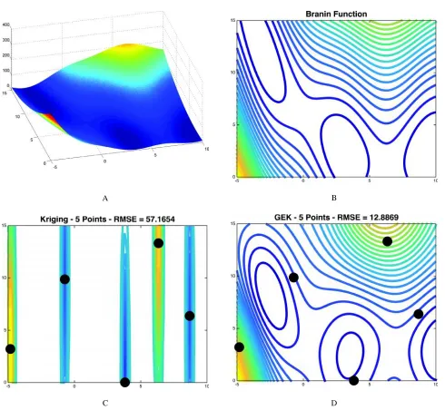
surrogate models are used to fit an analytical function with a set of sample points. The set of sample points is generated by a Latin Hypercube Sampling (LHS) method. The analytical function used for comparison is the 2-D Branin function described by Eq. (39). Surrogate models are used to fit the 2-D Branin function using 5 sample points generated by LHS. The gradient components are analytically evaluated on these sample points.
2
22 1 1
1
( )
(1 ) cos( )
f a x bx cx r
s t x s
x
(39)
The shape and contour of the 2-D Branin function (where a = 1, b = 5.1/42, c = 5/, r = 6, s =
10, and t = 1/8) is illustrated in Figs. 1(A)-1(B), respectively. In Figs. 1(C)-1(D), Kriging and Gradient-Enhanced Kriging surrogate models constructed on 5 data points are compared. The Gradient Enhaced Kriging model is constructed by the direct Kriging approach. Although the function values show agreement at the 5 sample locations, the conventional Kriging model cannot capture the global trend of the Branin function. By including the gradient information, the Gradient-Enhanced Kriging model reproduces the global trend very accurately. Thus, the Gradient-Enhanced Kriging model is promising for constructing an accurate surrogate hybrid bridge function for use in gradient-based optimization.
Hybrid Bridge Function (HBF)
One of the key issues for variable fidelity modeling (VFM) is how to manage the different models of varying fidelity, or how to correct the low-fidelity model to approximate the high-fidelity data by making
use of so-called “bridge functions”, which are sometimes called “scaling functions”. The existing
bridge functions can be divided into three categories (Gano, 2005):
· Additive · Multiplicative · Hybrid
of low-order polynomials, Kriging models, or any surrogate.
The multiplicative bridge function can be defined using Eq. (41). In Eq. (40), fH(x) and fL(x) denote the high and low-fidelity models, respectively. After the exact but unknown bridge function (x) has been approximated withˆ( )x , the high-fidelity model fH(x) can be approximated by the VFM using Eq. (41) (Han, 2013).
( ) ( )
( )
H
L
f f
x x
x (40)
MULT( ) ˆ( )fL( ) fH( )
x x x x (41)
It can be shown that the function (x) is the scaling ratio between the high-fidelity data and the low-fidelity model. When(x) is multiplied by the low-fidelity model, the response of the high-fidelity model is achieved. However, the above multiplicative bridge function may cause problems when one of the sampled values of the low-fidelity model is close to zero. In such a case, the values of both the high and low-fidelity models should be shifted to avoid error.
A B
Fig. 1: 2-D Branin function for surrogate comparison. (A) Visualization of 2-D Branin function, (B) Exact 2-D Branin function contour, (C) Kriging surrogate contour and (D) GEK surrogate contour
[image:10.612.64.554.72.524.2]To avoid the possible problem of dividing by zero when using multiplicative bride functions, an additive bridge function was developed. The additive bridge function can be expressed by Eq. (43). In Eq. (42),
fL(x) and fH(x) denote the low and high-fidelity models, respectively. After the exact but unknown bridge function (x) has been approximated with
ˆ( )
x , the high-fidelity model fH(x) can be approximated by the VFM using Eq.(43) (Choi, 2009).
(x) = fH(x) – fL(x) (42)
ADD( ) fL( ) ˆ( ) fH( )
x x x x (43)
It can be shown that the function (x) is essentially the error or difference between the low and high-fidelity models. When ˆ( )x is added to the low-fidelity model, the response of the high-fidelity model is obtained.
Gano showed that additive bridge functions are not always better than multiplicative ones. Both have merits and demerits. Hence, Gano et al. developed a hybrid method that combines the multiplicative and additive methods as shown in Eq. (44) (Gano, 2005).
MULT MULT
( ) ( ) (1 ) ( )
x x x (44)
In Eq. (44), is a weight coefficient. The determination of being the key point for the success of this hybrid bridge function. Eldred et al. proposed to use the previously evaluated point to adjust the value of as in Eq. (45).
ADD
MULT ADD
( ) ( )
( ) ( )
H old new
new new
f
x x
x x (45)
In Eq. (47), fH(xold) denotes the optimum of the previous optimization step. During the process of optimization, a new value can be computed at each iteration. Updating these weights allows the framework to adapt as the optimization process matures.
However, the problem becomes quite different for the construction of a VFM for aero-loads prediction, where a global model in a relatively large parameter space is sought after. There is no guarantee that the VFM will converge to the exact function if
the above method is used directly (Han, 2013). Therefore, a new method is proposed in this work for calculating these weighting coefficients. This method follows a Bayesian Model Averaging (BMA) approach that allows for the utilization of all data available within the trust region of the current subproblem optimization defined by the previously discussed TRMM methodology. This methodology defines the hybrid bridge function as the form of Eq. (46) (Kennedy, 2001).
MULT MULT ADD ADD
( ) ( ) ( )
x x x (46)
In Eq. (46), MULT and ADD are determined using Eqs. (47-48) respectively. It is worth nothing that calculation of these weighting coefficients in this manner allows for and adaptive approach to calculation of said coefficients given that the current coefficient is dependent upon the previous coefficients
where 0 0 1
2
MULT ADD
(Park, 2010 and Droguett, 2008).
1
1 1
( )
( ) ( )
k
k ADD ADD
MULT k k
MULT MULT ADD ADD
x
x x (47)
1
1 1
( )
( ) ( )
k
k ADD ADD
ADD k k
MULT MULT ADD ADD
x
x x (48)
In Eqs. (47-48),MULT(x) andADD(x) denote the model likelihoods of MULT(x) and ADD(x), respectively. These model likelihood values are determined using Eqs. (49-50) where n denotes the number of data points available within the current trust region, i signifies either the multiplicative or additive cases, and j represents the jth data point contained within the current trust region (Park, 2011 and Zhang, 2000).
2
2 ,
1
( ) exp
ˆ
2 2
n
i
i MLE
n
x (49)
21 2
,
( ) ( )
ˆ
n
H j i j
j i MLE
f
SSE n
x x (50)variance 2 ,
(i MLE). Therefore, in this formulation, the
weighting coefficients are adaptively updated using all available data contained within the kth subproblem optimization trust region.
Demonstraton Problem
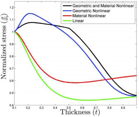
Consider a fixed titanium plate subject to a uniform temperature change of T = 1000oC depicted in Fig. 1.
This specific design problem is indicative of the real world scenario of a thermal exhaust washed structure, plate over which hot exhaust gasses flow. This problem, consists of 4 models, the first of which represents that of a low-fidelity model in which all governing physics are assumed to be linear. The second and third models assume that nonlinearity exist and include material and geometric nonlinear physics, respectively. The model which incorporates material nonlinearity is taken to be a lower-fidelity than that which incorporates geometric nonlinearity due to the assumption that geometric nonlinearities play a larger role in the stress response of the true system than material nonlinearities. Finally, the high-fidelity model is one in which both material and geometric nonlinearities are accounted for in the physics which drive the stress response. These fidelities are chosen to be used as demonstration of the multi-fidelity approach and proof of concept that this approach can be used on a set of pre-existing models.
Fig. 2 shows the normalized stress response of each of these 4 fidelities with respect to variation in plate thickness. This stress response is taken to be 2/ 3 the distance along the x-edge of the plate with origin in lower left-hand corner as shown by the red star in
Fig. 1. As can be observed, the two higher-fidelity models have opposing trends in comparison to the two lower-fidelity models. This specific scenario is the driving force behind the need for multi-fidelity design optimization rather than just a global surrogate which can fail in predicting the true high-fidelity sensitivity direction. It is assumed that the geometric and material nonlinear analysis most accurately represent the real world scenario given the understanding of physics involved.
Results
Engineering design often directly translates to performing optimization. The most common form of optimization used in engineering design is gradient based optimization. Gradient-based optimization is a mathematical technique in which a search direction for determining the best direction to perturb the design space is driven by the gradient of the objective (function of interest) at current design point. The optimization problem for the minimization of exhaust washed structure plate weight subject to a stress constraint is defined by Eq. (51).
Minimize: f(x) = Weight
Subject to: Edge stress – 60ksi < = 0
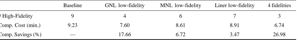
0.1 < t < 1 (51) For comparison, a baseline optimization was performed on the high-fidelity model using a traditional sequential quadratic programming optimization
Fig. 2: Thermal plate with quarter symmetric model shown
[image:12.612.317.550.523.720.2] [image:12.612.68.295.558.710.2]approach. This optimization took 9 high-fidelity function evaluations to reach an optimum of f(x) = 20.574 lbs at an optimum design point of x = 0. 5765 while strictly satisfying the stress constraint. The computational time required to converge to the high-fidelity optimum took approximately 9.23 minutes on a quad-core desktop computer clocked at 2.1 GHz with 16 GB of ram running windows 7 64-bit.
Implementation of the proposed multi-fidelity optimization technique was first carried out using each of the three lower fidelity models as the low-fidelity model in a two-level configuration. First,using the geometric and material nonlinear (GMNL) thermal model as the high-fidelity model and the geometric nonlinear (GNL) thermal model as the low fidelity model resulted in a computational savings of 17.66%. This optimization process required 4 high-fidelity and 7 low-fidelity function evaluations to reach an optimum of f(x) = 20.574 lbs at an optimum design point of x = 0. 5765 while strictly satisfying the stress constraint. The computational time required to converge to this optimum took approximately 7.60 minutes on a quad-core desktop computer clocked at 2.1 GHz with 16 GB of ram running windows 7 64-bit.
The second multi-fidelity optimization was performed using the geometric and material nonlinear (GMNL) thermal model as the high-fidelity model and the material nonlinear (MNL) thermal model as the low fidelity model resulting in a computational savings of 6.72%. This optimization process required 6 high-fidelity and 8 low-high-fidelity function evaluations to reach an optimum of f(x) = 20.574 lbs at an optimum design point of x = 0. 5765 while strictly satisfying the stress constraint. The computational time required to converge to this optimum took approximately 8.61 minutes on a quad-core desktop computer clocked at 2.1 GHz with 16 GB of ram running windows 7 64-bit.
The final two-level multi-fidelity optimization was performed using the geometric and material nonlinear
(GMNL) thermal model as the high-fidelity model and the linear thermal model as the low fidelity model. This optimization process required 7 high-fidelity and 28 low-fidelity function evaluations to reach an optimum of f(x) = 20.574 lbs at an optimum design point of x = 0. 5765 while strictly satisfying the stress constraint.The computational time required to converge to this optimum took approximately 8.91 minutes on a quad-core desktop computer clocked at 2.1 GHz with 16 GB of ram running windows 7 64-bitwhich resulted in a computational savings of 3.47%. The final multi-fidelity optimization involved a four-level optimization process. This four-level process posed challenges not present in the two-level multi-fidelity optimization. The first challenge was the manner in which each model was corrected. It is desired that each model be adjusted to represent the
high-fidelity model. However, each model can’t be
corrected directly to the high-fidelity model due to the collection of data at each level does not contain the high-fidelity model. Rather, each model is corrected to above corrected model. Therefore, the geometric nonlinear model is corrected to the geometric and material nonlinear model. Likewise. The material nonlinear model is corrected to the corrected geometric nonlinear model which has already been corrected to the geometric and material nonlinear model. The other challenge is to ensure that all high-fidelity information be available to each of the individual models for building correction models as well as evaluating hybrid weighting coefficients.
Optimization was performed on the four-level configuration using the technique developed in this research addressing the previous mentioned challenges. This optimization took 3 high-fidelity, 4 medium-high-fidelity, 4 medium-fidelity, and 7 low-fidelity function evaluations to reach an optimum of
f(x) = 20.574 lbs at an optimum design point of x = 0.
[image:13.612.69.549.675.740.2]5765 while strictly satisfying the stress constraint. The computational time required to converge to this
Table 1:
Baseline GNL low-fidelity MNL low-fidelity Liner low-fidelity 4 fidelities
# High-Fidelity 9 4 6 7 3
Comp. Cost (min.) 9.23 7.60 8.61 8.91 6.74
optimum took approximately 6.74 minutes on a quad-core desktop computer clocked at 2.1 GHz with 16 GB of ram running windows 7 64-bit. Note that this optimum, as well as the optimums reached via the two-level multi-fidelity optimizations, is the same optimum reached by the baseline comparison optimization problem. Thus, the proposed multi-fidelity
optimization converges to the “true” high-fidelity
optimum. Therefore, implementing this multi-fidelity optimization methodology reduced computational cost
by while still converging to the ‘’true’’ (high-fidelity)
optimum. A summary of these results are tabulated in Table 1.
Conclusion
In this work, an adjustment factor technique (surrogate-based hybrid bridge function) combined with a Trust Region Model Management optimization scheme is presented for use in multi-fidelity design processes. The hybrid bridge function is a weighted average of additive and multiplicative adjustment
factors as shown by Fischer and Grandhi in (Fischer, 2014). The weighting coefficients are calculated using a Bayesian Model Averaging technique used in model-form uncertainty quantification. The key to the presented surrogate-based adjustment factor technique is the use of a Gradient-Enhanced Kriging (or Ordinary Kriging) surrogate model constructed over a localized trust region as shown previously by Fischer and Grandhi in (Fischer, 2014 and 2015). This localized trust region is adaptive in the sense that its relative size and location are determined by the accuracy of the corrected low-fidelity model through a Trust Region Model Management scheme. Therefore, a surrogate hybrid bridge function model is constructed utilizing all data available within the trust region (from previous optimization iterations) and the adjustment factors obtained at said points. These surrogate hybrid bridge functions are then utilized to correct low-fidelity simulation responses; thus, more accurately predicting a high-fidelity response.
References
Alexandrov N M, Lewis R M, Gumbert C R, Green L L and Newman P A (2001) Approximation and model management in aerodynamic optimization with variable-fidelity models Journal of Aircraft 38 1093-1101
Allaire D and Willcox K (2010) Surrogate modeling for uncertainty assessment with application to aviation environmental system models AIAA Journal 48 1791-1803
Chernoff H and Moses L E (2012) Elementary decision theory Courier Dover Publications New York
Choi S, Alonso J J and Kroo I M (2009) Two-level multifidelity design optimization studies for supersonic jets Journal of Aircraft 46 777-790
Droguett E L and Mosleh A (2008) Bayesian methodology for model uncertainty using model performance data Risk Analysis 28 1457-1476
Fadel G and Cimtalay S (1993) Automatic evaluation of move-limits in structural optimization Structural Optimization 6 233-237
Fischer C C and Grandhi R V (2014) Utilizing an adjustment factor to scale between multiple fidelities within a design process: A stepping stone to dialable fidelity design 16th AIAA Non-Deterministic Approaches Conference Sci Tech 2014 A14-1011 National Harbor Maryland January 2014
Fischer C C and Grandhi R V (2015) A surrogate-based adjustment factor approach to multi-fidelity design optimization 17th AIAA Non-Deterministic Approaches Conference SciTech 2015A15-1375 Kissimmee Florida January 2015 Forrester A I J, Sobester A and Keane A J (2007) Multi-fidelity
optimization via surrogate modelling Proc R Soc A 463 3251-3269
Forrester A, Sobester A and Keane A (2008) Engineering design via surrogate modelling: A practical guide John Wiley & Sons New York
Gano S E, Rnaud J E and Sanders B (2005) Hybrid variable fidelity optimization by using a Kriging-based scaling function AIAA Journal 43 2422-2433
Han Z H and Zhang K S (2012) Surrogate-based optimization intec book real-world application of genetic algorithm InTech 343-362
Han Z H, Gortz S and Zimmermann R (2013) Improving variable-fidelity surrogate modeling via gradient-enhanced kriging and a generalized hybrid bridge function Aerospace Science and Technology 25 177-189
Jones D R 2001A taxonomy of global optimization methods based on response surfaces Journal of Global Optimization
Jones D R, Schonlau M and Welch W J (1998) Efficient global optimization of expensive black-box functions Journal of Global Optimization 13 455-492
Kennedy M C and O’Hagan A (2001) Bayesian calibration of
computer models Journal of the Royal Statistical Society: Series B (Statistical Methodology) 63 425-464
Lewis R M (1996) A trust region framework for managing approximation models in engineering optimization Sixth AIAA/NASA/ISSMO Symposium on Multidisciplinary Analysis and Design A96-4101 Reston Virginia September 1996
Lewis R M and Nash S G (2000) A multigrid approach to the optimization of systems governed by differential equations 8th Symposium on Multidisciplinary Analysis and Optimization A00-4890 Long Beach California September 2000
Liu W (2003) Development of gradient-enhanced kriging approximations for multidisciplinary design optimization PhD Thesis – University of Notre Dame
Lockwood B and Anitescu M (2011) Gradient-enhanced universal kriging for uncertainty propagation in nuclear engineering Transactions of the American Nuclear Society 104 347
Lockwood B and Mavriplis D (2013) Gradient-based methods for uncertainty quantification in hypersonic flows Computers & Fluids 85 27-38
March A and Wilcox K (2012) Provably convergent multifidelity optimization algorithm not requiring high-fidelity derivatives AIAA Journal 50 1079-1089
Park I and Grandhi R V (2011) Quantifying multiple types of uncertainty in physics-based simulation using Bayesian model averaging AIAA Journal 49 1038-1045
Park I, Amarchinta H K and Grandhi R V (2010) A Bayesian approach for quantification of model uncertainty Reliability Engineering & System Safety 95 777-785
Robinson T, Eldred M, Willcox K and Haimes R 2008 Surrogate-based optimization using multifidelity models with variable parameterization and corrected space mapping AIAA Journal 46 2814-2822
Yamazaki W and Marvriplis D J (2013) Derivative-enhanced variable fidelity surrogate modeling for aerodynamic functions AIAA Journal 51 126-137