Sensitivity of Lagrangian Particle Tracking Based on a 3D Numerical Model

Sensitivity of Lagrangian Particle Tracking Based on

a 3D Numerical Model

Dang Huu Chung, Nguyen Thi Kieu Duyen

Institute of Mechanics, Vietnamese Academy of Science and Technology, Hanoi, Vietnam Email: [email protected], [email protected]

Received October 1,2012; revised November 1, 2012; accepted November 9, 2012

ABSTRACT

The aim of the paper is to investigate in detail the sensitivity of particles displacement based on method of Lagrangian particle tracking in combination with a 3D Eulerian numerical model that was developed by the first author, namely FSUM. The characteristic parameters used for this research include the possibilities of random movement, settling ve-locity of solid particle, horizontal and vertical diffusion coefficients and condition of particle fixed with a constant dis-tance under water surface. The first part is on the fluid flow model. It includes 3D Navier-Stokes equations together with the initial and boundary conditions that were numerically solved with the finite difference method and coded with FORTRAN 90/95 using parallel technique with OpenMP. A semi-Lagrangian treatment of the advective terms was used. The second part is related to Lagrangian particle tracking model and was solved with the fourth Runge-Kutta method. Model was applied for Strait of Johor and has been calibrated by using measured data on water level and velocity at one station. Eight cases of simulations with many different options were carried out. Through computed cases it shows that random term and settling velocity are very important factors for the behavior of particle trajectory. Although the ran-dom diffusion is minor in comparison with flow velocity, but it can rearrange the initial distribution of particles then the cluster of particles become more dispersive during the process of movement. In addition, introducing settling velocity of particle makes a big change on the trajectory of particle that becomes more suitable to sediment transport. The study gave a comprehensive picture on particle movement. The model also showed its possibilities of multiform applications in simulation and prediction for the different problems in practice.

Keywords: 3D FSUM Model; Random Walk; Settling Velocity; Numerical Simulations

1. Introduction

The idea of study on the trajectories of movement for solid particles in fluid environment appeared very early in mechanics and was considered as the movement in Lagrangian point of view. The advantage of this method is that it is possible to track the process of movement for each specific particle in more detail and accuracy in comparison with the method of determining average concentration for grid cells through the advection-diffu- sion equation based on Euler point of view. However, the numerical solution is too difficult to implement in prac-tice when the number of particles is very large, because it strongly depends on the speed of computer machine pro-cessor as well as a very large amount of memory to be distributed for the variables. Fortunately, nowadays the development of Information technology both on hard-ware and softhard-ware is considerable and such a problem is completely possible to be solved quickly event on PC, especially with parallel technique. There are many stud-ies on this problem for different applications so far, such as study on contaminant transport [1,2], study on

sus-pended sediment transport [3], study on transport in het-erogeneous porous media [4-7], or study on prediction of oil slick transport in the sea [8], etc.

In general the real movement of solid particles includes two parts [1]: one by the advection of fluid flow and the other one by the “random walk”. So a fluid dynamics model is necessary to couple for velocity field generation.

In this paper the module of Lagrangian particle track-ing is developed and incorporated into FSUM (Flows with Substance transport and bed Morphology) devel-oped by Chung, D.H. [9] as an effective tool to solve many problems in fluid dynamics raised from practice as mentioned above.

The paper concentrates on the mathematical equations, numerical simulation, especially some sensitive factors related to orbits of particles and the possibility of model application.

2. Mathematical Model for Lagrangian

Particle Tracking

As mentioned above the movement of particles includes

, h v s s two parts, in which the first part is related to fluid

veloc-ity field that is governed by Reynolds-averaged Navier- Stokes equations together with initial and boundary con-ditions [9,10] as follows:

0

  V (1)





2

1 h v

xy

t

p  

              V V V V z z  _{  }       V F  (2)













, , 0, , ,

x y z

t x y z



  

V



, , , 0, ,

x y z t G

 

0, (3)



0, x y z, ,   L, t 0





 

V n , (4)



x y z t, , ,



 f₁ x y z t, , , ,



x y z, ,



   , t 0

 , (5)

 





_,



_{, ,}



_,

, 0

,

, w w

x y v u v

x y z G

z z t          

 

  

, (6)

 





2 2

2 ,

, , , , ,

v u v g u v _{u v x y z G}

     

, 0

b

z C

z z t

    

, ,

(7)

in which t is the time, x y z





T

, , u v w



V

the spatial coordinates, the velocity vector of fluid flow,



fv



 





0,0,

T

, fu,0



T

the Coriolis acceleration vector, g

 

F , g the acceleration of gravity,  the water density, the non-hydrostatic pressure, p  h, v the horizontal and vertical momentum diffusion coeffi-cients, f1 _{the given function of water level at open}

boundary, the solution domain, the land bound-ary, _{the lateral open boundary,} C Chezy coefficient,

the normal vector, G

, w w

L



n  x y the shear stress compo-nents on water surface by wind and b the bed bathym-etry with the downward positive direction.

z

The second part is related to Lagrangian particle tracking model and it is also described as a “random walk”. For this kind of problem it is expected to deter-mine the accurate location for each particle



x y z, ,





, ,

with the initial condition



x y z0 0 0 rather than the propagation of cell-average concentration. The differen-tial equations for the Lagrangian movement of particles [11] are as follows:





drift ran

d d d d 6 d 2h 1

x x  x u t  t r (8)





6 d 2h 1

t r



 

drift ran

dydy dy v td (9)







drift ran

d d d d 6 d 2v

s

z z  z  ww t  t r1



(10)

in which d ,d ,dx y z

t

are the spatial displacements of a particle after a time step d , w settling velocity of

particle,  

1 1 1

1/ 2 1/ 2 1/ 2 1/ 2

1 1

1/ 2 1/ 2 1/ 2 1/ 2

n n n

ij ij xi j i j xi j i j

n n

yij ij yij ij ij

d s s

s s b

                           



1



1/ 2 _{1/ 2}

n T

xi j x

i j

s _  Z A Z



  



1



1/ 2 _{1/ 2}

n T

yij y

ij

s _  Z A Z



  

1/ 2 1/ 2 1/ 2 1/ 2

1

ij xi j xi j yij yij

d s  s  s  s 

the horizontal and vertical diffusion coefficients and r is a random number from a normally distributed random variable in [0, 1].

It should be noted that the factor of 2r − 1 in the ran-dom terms on the right hand sites of the Equations (8)-(10) have a mean of zero and a variation range from –1 to 1. This range allows the particles to move about the new position due to advection term that is more suitable for real movement of particles in practice. In addition, the inclusion of settling velocity of particle allows movement of particles of different physical features to be taken into account. It covers the possibility of settling and reduction of particle quantity in the process of movement. In case of using the settling velocity of particle in condition of very high temperature-salinity gradients it should be noted that when the temperature increases or the salinity decreases, the water density and viscosity decrease as well, hence the relative density of the particles increases resulting in an increase of the settling velocity of the par-ticles [12].

3. Numerical Method for Governing

Equations

The Equations (1) and (2) together the initial and bound-ary conditions were numerically solved in FSUM [9,10] with the finite difference method and coded with FOR-TRAN 90/95. Approach of operator splitting for the fi-nite-difference equations combining a semi-Lagrangian treatment of the advective terms with a semi-implicit discretization of the vertical diffusion terms is used [13, 14]. The continuity Equation (1) is integrated vertically from bottom to the surface and then it is discretized for water level difference equation. By eliminating the ve-locity components from this one, a penta-diagonal equa-tion system is obtained ([15]):

(11)

,

    

















T 1 T 1

1/2 1/2

T 1 T 1

1/2 1/2

n n

n

ij ij x _{i j} x _{i j}

n n

y _ij y _ij

b Z A G Z A G

Z A G Z A G

                      1 n in which ij

, ,

is water level at time step n + 1 for hy-drostatic pressure;    x y x y are the expressions depending on grid size and time step; ij

n

thick-ness, _{vector related to the right hand site of Equation} (2) excluding vertical component of velocity gradient and values interpolated on the characteristics,

G

A _tri-diago-

nal matrix containing vertical layer thickness, time step and boundary conditions of velocity on water surface and on bottom.

Equation (11) is solved first with the conjugate gradi-ent method. After that the equations for velocity compo-nents are calculated by solving a linear equation system for vertical cells. It should be noted that method of in-verse matrix was effectively applied for this situation in FSUM, because these vectors _A1_Z

and A G1 _had been calculated and stored during determining the coeffi-cients for the penta-diagonal equation system of water level. If the assumption of non-hydrostatic is used the next step for non-hydrostatic correction will be imple-mented. The detail for solving Navier-Stokes is beyond the scope of this paper.

In order to solve the equations for Lagrangian particle tracking (Cauchy problem for ordinary differential equa-tions), the fourth order Runge-Kutta ([16]) is used, be-cause this method is simple but gives a quite high accu-racy. The treatments of particles at land and open bound- aries are based on a purely mathematical method. When a particle moves over the land boundary, it will be put back to the previous location without consideration of decay phenomenon for this study. When a particle moves through the open boundary, it will be removed out the list of particles under consideration. The mathematical for-mulae of the fourth order Runge-Kutta for the Equations (8)-(10) are as follows:









1 11 2 K122 13 14



6

6 d 2 1

n n

h

x x K K K

t r



        

 



(12)





1 21 22

6 d 2 1

n n

h

y y K

t r



      

 

23 24 6

K K

  



2 K 2



(13)





1 31 2 K32 2 K33 K34 6



6 d 2 1

n n

v

z z K

t r



       

  (14)

in which K_ij i1,3;j1,4



are determined accord-ing to the values at previous time. In order to speed up the process of computation in FSUM a parallel technique by using OpenMP [17] was applied and it is an optional choice in case of need.

4. Model Application

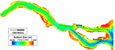
[image:3.595.310.539.86.186.2]

The computation domain for Lagarangian particle track-ing application is the eastern part of the Strait of Johor (Malaysia). It is separate from the western part by the causeway (Figure 1). The domain is covered by a rec-tangular grid with grid size    x y 90 m including

Figure 1. Eastern Strait of Johor (Station STN4 and release location).

8346 active grid cells in the horizontal plan. The vertical datum used for this hydrodynamic study is based on the Mean Sea Level (MSL). The lowest bottom elevation under the datum is about 24 m, therefore a 3D model with 10 vertical layers is reasonable. The domain has only one open boundary on the right of the Strait of Johor, while the left boundary is closed by the causeway. The boundary condition is water level predicted from the harmonic constants of Sungai Segget with a tidal range of about 3 m. Model set-up is easily carried out with EFDC_Explorer, a useful tool developed by Craig P M [18] for EFDC [19].

In order to study on the movement of particles, a group of 100 particles was released at the location (see Figure 1) around the geography coordinates of (103.98˚E, 1.40˚N) at the same time. It is concentrated on 8 cases with many different options (Table 1), in which case 3D-01 is con-sidered as the standard to recognize the difference of the other cases. There are four options for random movement of particle: horizontal only; vertical only; both horizontal and vertical (full 3D) and without random movement. The coefficients of horizontal and vertical diffusion used in this study are constants. The possibility of free move-ment or restricted movemove-ment of particles by a fixed depth under water surface is also considered. The settling ve-locity of particles is also taken into account to see its impact on behavior of particle trajectory for suspended sediment transport study that is one of application fields of Lagrangian particle tracking model. The settling ve-locity is calculated from the following formula ([20]):



_{2 3}



1 2

50

10.36 1.049 s

w d



 10.36 D

 _ 

 _  _ (15)

 

d

in which 50 the median grain diameter,  the

kine-matic viscosity and D dimensionless grain size. So the settling velocity of case 3D-02 is corresponding to fine sand (d50100 μm) and the one of 3D-03 is for

coarse sand (d50300 μm). This parameter is ignored in

other cases. Case 3D-04 is the situation without random movement. This means that the particle is only carried away by flow current. Case 3D-05 is a special case, in which particle movement is restricted by a condition that

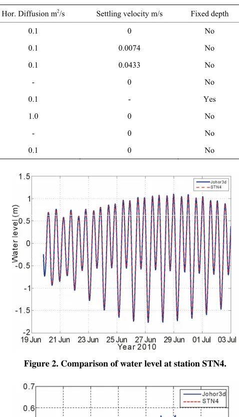
[image:3.595.75.289.461.580.2]

[image:4.595.298.537.98.514.2]

Table 1. Options for Lagrangian particle tracking model.

Case Random movement Ver. Diffusion m2_{/s Hor. Diffusion m}2_{/s Settling velocity m/s Fixed depth}

3D-01 Horizontal - 0.1 0 No

3D-02 Horizontal - 0.1 0.0074 No

3D-03 Horizontal - 0.1 0.0433 No

3D-04 No - - 0 No

3D-05 Horizontal - 0.1 - Yes

3D-06 Horizontal - 1.0 0 No

3D-07 Vertical 0.01 - 0 No

3D-08 Full 3D 0.01 0.1 0 No

the distance of particle under water surface is fixed (such as application for oil slick prediction). Case 3D-07 is used to consider the effect of vertical diffusion only and the last case is more complete on influence of random factor (full 3D).

5. Results of Simulation

The application of FSUM model includes two steps, in which the first step is the calibration of the model in re-spect of hydrodynamics based on the measured data of water level and velocity at the station STN4 located at (103.94˚E, 1.43˚N) for a period from June 20 to July 2, 2010 (Figure 1).

The comparison of measured and computed water lev-el is presented in Figure 2. It shows that the water levlev-els of computation and measurement fit well. The velocity intensity and direction at the height of 8.9 m above bot-tom are presented in Figures 3 and 4. In general it is seen that the time series of computed velocity are suitable for measured data on phase, intensity and direction as well.

Figure 2. Comparison of water level at station STN4.

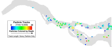
The second step is the application of FSUM to simu-late particle movement for 8 different cases as described in Table 1. Figures 5-12 show the horizontal and verti-cal distributions and the tendency of dispersion of parti-cles in a plan view over 10 days. Figure 5 is considered a typical tendency of particle movement under the action of advection, horizontal diffusion and random displace-ment without any constraint at the water surface. From Figures 6 and 7 it is clearly seen that the movement of particles is more concentrated than other cases. This is due to the impact of settling velocity of particle and the vertical profile of flow velocity. In these cases right after being released the particles quickly fell down to the layer close to the bottom where velocity is quite small. Figure 8 represents the simulation result of case 3D-04. When the random term is ignored the split of particles is de-layed for a period of time. Since they were very close together and were released at the same time, therefore the

Figure 3. Comparison of velocity intensity at station STN4.

influence of flow on the particle movement is not really different at the first stage. Then the particles gradually disperse due to horizontal velocity field.

[image:4.595.53.542.101.258.2] [image:4.595.312.532.477.652.2]

is clear that all of particles have nearly the same eleva-tion at a time moment and their dispersion is less than case 3D-01. This is completely reasonable, because the

[image:5.595.312.534.87.182.2]

Figure 4. Comparison of velocity direction at station STN4.

[image:5.595.59.284.136.303.2]

Figure 5. Status of particle over 10 days (case 3D-01).

Figure 6. Status of particle over 10 days (case 3D-02).

[image:5.595.315.535.217.311.2]

Figure 7. Status of particle over 10 days (case 3D-03).

[image:5.595.60.289.342.442.2]

Figure 8. Status of particle over 10 days (case 3D-04).

[image:5.595.308.536.353.443.2]

Figure 9. Status of particle over 10 days (case 3D-05).

Figure 10. Status of particle over 10 days (case 3D-06).

Figure 11. Status of particle over 10 days (case 3D-07).

Figure 12. Status of particle over 10 days (case 3D-08).

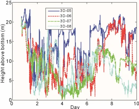
[image:5.595.312.536.485.577.2] [image:5.595.61.287.615.713.2] [image:5.595.311.535.616.711.2]

particles were fixed under water surface with a constant distance and the random displacement is ignored, there-fore they were not affected by vertical profile of velocity. So this suggests that random factor is a very important quantity for particle dispersion. Case 3D-06 is presented in Figure 10 and shows that the greater diffusion coeffi-cient is the more separate particles are. The dispersion of particles is the strongest in this case, because the coeffi-cient of horizontal diffusion now becomes considerable in each differential equations for x and y. The impact of vertical diffusion can be ignored through the comparison between cases 3D-04 (Figure 8) and 3D-07 (Figure 11). This remark is also suitable to case 3D-08 for both hori-zontal and vertical diffusion. The result of this case is not really different with case 3D-01. This means that random movement in the vertical direction is not as important as random movement in the horizontal plan. Figures 13 and 14 give more information on particle heights above bot-tom versus time. It can be seen that for only cases 3D-02 and 3D-03 the particle 1 quickly moved downward to bottom and traveled closely on bottom for whole the time of simulation. The behaviors of particle movement of these cases are quite similar with sediment transport, therefore Lagrangian particle tracking model with set-tling velocity taken into account is very suitable for sediment transport simulation. For the other cases with-out settling velocities the elevations of particles mainly depend on the water surface elevation during flood or ebb tide.

6. Conclusions

[image:6.595.310.534.86.262.2]

The hydrodynamic variables generated by FSUM in-cluding water depth and velocity field were carefully calibrated with data set from measurement. This can be used as more verification for the reliability of FSUM both on algorithm and its application to practice. The

Figure 13. Height above bottom of particle N.1 versus time.

Figure 14. Height above bottom of particle N.1 versus time.

previous verification was carried out by using data from wave flume and some computed domains with very complicated geometries. In general, so far all of applica-tions showed that the results computed with FSUM are quite stable and reliable. In this study through 8 cases of simulation for Lagrangian particle tracking with many different options on random term, diffusion coefficient, settling velocity and fixed distance of particles under water surface some interesting remarks were obtained. These give us more understanding on behavior of particle movement in fluid environment by a combination be-tween Eulerian and Lagrangian descriptions.

First of all, it is obvious that the trajectory of a particle strongly depends on the field of flow velocity as known. However, the random action in fluid flow also plays a very important role. Although the random diffusion is minor in comparison with flow velocity, but it can rear-range the initial distribution of particles then they gradu-ally separate and are carried away by flow current, therefore the cluster of particles become more dispersive. In respect of numerical simulation, this also suggests that the Lagrangian particle tracking model should be started when the hydrodynamic model becomes stable in order to avoid the inaccuracy due to the initial conditions for velocity field.

Also from the computed results it can be seen that the particles at the same elevation will move together in a cluster, while the particles located in a large vertical dis-tance have the tendency to move more and more sepa-rately due to vertical profile of velocity. In addition, dif-fusion coefficient also contributes an important part to this tendency.

[image:6.595.57.284.540.719.2]

Copyright © 2012 SciRes. JMP coast zones if a suitable parameterization is well done. In

this case after a particle is released, it quickly moves downward to the layer close to bottom and its travel length becomes shorter. Sometimes, it settles on bed de-pending on the strength flow velocity. In this situation movement of particle is quite similar to that of bed-load transport.

Finally, Langrangian particle tracking model can be one of the prospective approaches for further applications in future when the ability of memory and speed of com-putation of PC are not the real issues.

7. Acknowledgements

This study was funded by NAFOSTED. The authors would like to thank Dr. Baharim from UTM for the measured data on velocity at the station STN4 and the harmonic constants of Sungai Segget. At the same the first author also would like to express his deep gratitude to Mr. Craig for many things he did. Many thanks are sent to Mr. Scandrett for his useful help.

REFERENCES

[1] W. E. Hathorn, “Simplified Approach to Particle Track-ing Methods for Contaminant Transport,” Journal of Hy-draulic Engineering, Vol. 123, No. 12, 1997, pp. 1157- 1160. doi:10.1061/(ASCE)0733-9429(1997)123:12(1157) [2] C. F. Scott, “Particle Tracking Simulation of Pollutant

Discharges,” Journal of Environmental Engineering, Vol. 123, No. 9, 1977, pp. 0919-0927.

[3] N. J. MacDonald, et al., “Particle Tracking Model Report 1: Model Theory, Implementation, and Example Applica-tions,” Working Paper, US Army Engineer Research and Development Center, ERDC/CHL TR-06-20, 2006. [4] C.-H. Park, et al., “A Study of Preferential Flow in

Het-erogeneous Media Using Random Walk Particle Track-ing,” Geosciences Journal, Vol. 12, No. 3, 2008, pp. 285- 297. doi:10.1007/s12303-008-0029-2

[5] A. E. Hassan and M. M. Mohamed, “On Using Particle Tracking Methods to Simulate Transport in Single-Con- tinuum and Dual Continua Porous Media,” Journal of Hydrology, Vol. 275, No. 3-4, 2003, pp. 242-260. doi:10.1016/S0022-1694(03)00046-5

[6] E. M. LaBolle, G. E. Fogg and A. F. B. Tompson, “Ran-dom Walk Simulation of Transport in Heterogeneous Po-rous Media: Local Mass-Conservation Problem and Im-plementation Methods,” Water Resources Research, Vol. 32, No. 2, 1996, pp. 583-593. doi:10.1029/95WR03528 [7] P. Salamon, “On Modeling Contaminant Transport in

Com-plex Porous Media Using Random Walk Particle Track-ing,” Ph.D. Thesis, Instituto de Ingenieria del Agua y

Medio Ambiente Universidad Politecnica de Valencia, 2006.

[8] K. A. Korotenko, et al., “Particle Tracking Method in the Approach for Prediction of Oil Slick Transport in the Sea: Modeling Oil Pollution Resulting from River Input,” Journal of Marine Systems, Vol. 48, No. 1-4, 2004, pp. 159-170. doi:10.1016/j.jmarsys.2003.11.023

[9] D. H. Chung, “On FSUM Model and Application,” Viet-nam Journal of Mechanics, Vol. 30, No. 4, 2008, pp. 237- 247.

[10] D. H. Chung, “Numerical Simulation of Sediment Trans-port from Ba Lat Mouth and the Process of Coastal Mor-phology,” Journal of Geophysics and Engineering, Vol. 5, No. 1, 2008, pp. 46-53. doi:10.1088/1742-2132/5/1/005 [11] D. W. Dunsbergen and G. S. Stalling, “The Combination

of a Random Walk Method and a Hydrodynamic Model for the Simulation of Dispersion of Dissolved Matter in Water,” Transactions on Ecology and the Environment Vol. 2, WIT Press, 1993.

[12] D. H. Chung, “Effects of Temperature and Salinity on the Suspended Sand Transport,” International Journal of Nu-merical Methods for Heat & Fluid Flow, Vol. 17, No. 5, pp. 512-521.doi:10.1108/09615530710752973

[13] V. Casulli and G. S. Stelling, “Numerical Simulation of 3D Quasi-Hydrostatic, Free-Surface Flows,” Journal of Hydraulic Engineering, Vol. 124, No. 7, 1998, pp. 678- 698. doi:10.1061/(ASCE)0733-9429(1998)124:7(678) [14] D. H. Chung and D. Eppel, ‘‘Effects of Some Parameters

on Numerical Simulation of Coastal Bed Morphology,” International Journal of Numerical Methods for Heat & Fluid Flow, Vol. 18, No. 5, 2008, pp. 575-592.

doi:10.1108/09615530810879729

[15] H. Kapitza, “TRIM Documentation Manual,” Working Paper, GKSS Institute for Coastal Research, 2001. [16] J. D. Hoffman, “Numerical Methods for Engineers and

Scientists,” McGraw-Hill International Edition, 2001. [17] M. Hermanns, “Parallel Programming in FORTRAN 95

using OpenMP,” Working Paper, School of Aeronautical Engineering, Universidad Politécnica de Madrid, Madrid, 2002.

[18] P. M. Craig, “User’ Manual for EFDC_Explorer: A Pre/ Post Processor for the Environmental Fluid Dynamics Code,” Working Paper, Dynamic Solutions-International, Knoxville, 2011.

[19] J. M. Hamrick, “A Three Dimensional Environmental Fluid Dynamics Computer Code: Theoretical and Computational Aspects,” Working Paper, The College of William and Mary, Virginia Institute of Marine Science, Special Re-port, Vol. 317, 1992, p. 63.