A novel technique for a class of singular boundary value problems
Mohammad Hadi Noori Skandari∗ Faculty of Mathematical Sciences,
Shahrood University of Technology, Shahrood, Iran. E-mail: [email protected]
Mehrdad Ghaznavi
Faculty of Mathematical Sciences,
Shahrood University of Technology, Shahrood, Iran. E-mail: [email protected]
Abstract In this paper, Lagrange interpolation in Chebyshev-Gauss-Lobatto nodes is used to develop a procedure for finding discrete and continuous approximate solutions of a singular boundary value problem. At first, a continuous time optimization problem related to the original singular boundary value problem is proposed. Then, using the Chebyshev-Gauss-Lobatto nodes, we convert the continuous time optimization problem to a discrete time optimization problem. By solving the discrete time op-timization problem, we find discrete approximations for the solutions of the main singular boundary value problem. Also, by Lagrange interpolation we obtain a con-tinuous approximation for the solution. The efficiency and reliability of the proposed approach are tested by solving three practical singular boundary value problems.
Keywords. Singular boundary value problem, Chebyshev polynomial, Continuous time optimization
prob-lem, Discrete otimization problem.
2010 Mathematics Subject Classification. 34B16, 90C30.
1. Introduction
Consider the following singular boundary value problems (SBVPs)
y′′(t) +P(t)
R(t)y
′(t) =f(t, y(t)), 0≤t≤1, (1.1)
subject to the boundary conditions
y′(0) = 0, αy′(1) +βy(1) =γ, (1.2)
whereα, βand γare nonnegative constants. We assume thatR(0) = 0, R(t)̸= 0 for
t̸= 0 andP(0)̸= 0.Moreover, we suppose thatf(·,·) is continuous and ∂f∂t(·,·) exists and it is continuous on the domain [0,1].
Received: 10 May 2017 ; Accepted: 2 December 2017.
∗Corresponding author.
The singular boundary value problem (1.1)-(1.2) arises in a number of applications such as gas dynamics, nuclear physics, chemical reactions, atomic calculations, tumor growth and physiology. For example, SBVP (1.1)-(1.2) withP(t) = 2, R(t) =tand
f(t, y(t)) = ny(t)
y(t) +k, n, k >0,
occurs in the modeling of steady state oxygen in a spherical cell with Michaelis-Menten uptake kinetics [25,26]. In the study of various tumor growth problems [1–4,6], we deal with the SBVP (1.1)-(1.2) withP(t) = 0,1,2, R(t) =t and
f(t, y(t)) =h(y(t)) + ny(t)
y(t) +k, n, k >0.
Another case of physical significance is whenP(t) = 2, R(t) =tand
f(t, y(t)) =−le−lky(t), l, k >0,
which arises in the study of the distribution of heat sources in human head [12,15]. The singular boundary value problems have been the central attention to many research works either numerical or analytical [7–9,15–18,21–25,31–33]. The main dif-ficulty of the SBVP (1.1)-(1.2) is that the singularity behavior occurs att= 0.Various efficient numerical techniques have been used to deal with such SBVPs. For instance, Kumar [22] proposed a three-point finite difference method based on uniform mesh for a class of SBVPs. Benko et al. [5] utilized a backward Euler method for the nu-merical approximation of the solutions of singular second-order differential equations. Kanth and Reddy [19] studied fourth-order finite difference method to solve singular boundary value problems. Moreover, Kanth and Reddy [20] applied cubic spline in-terpolation method to solve these problems. Caglar and Caglar [7] utilized a method based on cubic B-spline method. Goh et al. [14] treated SBVPs by using quartic B-spline approximation where the values of coefficients are chosen via optimization. Zhang [34] proposed a modified cubic B-spline solution for two point boundary value problems. Moreover, variational iteration method [32,33], Adomian decomposition method [21], and modified Adomian decomposition method [24] are newly developed approximation methods that are applied to deal with such problems. In some of the mentioned methods the accuracy of the obtained solutions is poor while in the rest, implementation of the proposed approach is hard and time-consuming.
Now, in this paper, a method based on the Lagrange interpolation is proposed to solve the SBVP (1.1)-(1.2). Firstly, a continuous time optimization (CTO) problem related to the main SBVP is proposed. Then, applying the Chebyshev-Gauss-Lobatto (CGL) nodes, we convert the CTO problem to a discrete time optimization problem. The proposed approach is implemented on some numerical examples and the accuracy of the method is compared with some other well-known approaches. Obtained results, show the high accuracy of the method in comparison with the other methods.
2. The proposed approach
Lagrange interpolation in CGL nodes is important in approximation theory, since the roots of the Chebyshev polynomials of the first kind, also called CGL nodes, are used as nodes in polynomial interpolation and the resulting interpolation polynomial provides an approximation that is close to the polynomial of the best approximation of a continuous function under the maximum norm.
Here, we interpolate the solution in the roots of the Chebyshev polynomials to give the best accuracy in the interpolation of solution. The derivatives of these interpo-lating polynomials at these points are given exactly by a differentiation matrix. The similar approach was utilized in works [10,11,13,28–30].
In this section, at first, we apply a continuous time optimization (CTO) problem the optimal solution of which is a solution of SBVP (1.1)-(1.2). Thereafter, using the roots of the Chebyshev polynomials, we discretize the state variable of the CTO problem in CGL nodes and obtain a discrete-time optimization (DTO) problem. By solving the DTO problem, we obtain pointwise approximations for the solutions of SBVP (1.1)-(1.2). Moreover, by interpolating, we get continuous approximations for the solutions of the main problem.
According to the assumptions, we can convert the SBVP (1.1)-(1.2) to the following equivalent singular boundary problem
R(t)y′′(t) +P(t)y′(t) =R(t)f(t, y(t)), 0≤t≤1, (2.1)
subject to the boundary conditions
y′(0) = 0, αy′(1) +βy(1) =γ. (2.2)
In order to solve the SBVP (2.1)-(2.2), we propose the following continuous time optimization (CTO) problem
M inimize J =y′(0)2+ (αy′(1) +βy(1)−γ)2
subject to {
R(t)y′′(t) +P(t)y′(t) =R(t)f(t, y), 0≤t≤1. (2.3)
It is trivial that if SBVP (2.1)-(2.2) has a solutiony(.),theny(.) is an optimal solution for (2.3), and vice versa. Therefore, by solving the CTO problem (2.3), we can find the solution of SBVP (2.1)-(2.2).
Assume that y1(t) = y(t) and y2(t) = y′(t). So, the CTO problem (2.3) can be written as follows
M inimize J =y2(0)2+ (αy2(1) +βy1(1)−γ)2
subject to {
y′1(t) =y2(t),
R(t)y2′(t) +P(t)y2(t) =R(t)f(t, y1(t)), t∈[0,1].
To utilize the roots of Chebyshev polynomials (or CGL nodes), defined on the interval [−1,1], the transformationt= 12(τ+ 1) must be used. Moreover, we define
Y1(τ) =y1(τ+12 ) =y1(t), Y2(τ) =y2(τ+12 ) =y2(t),
Y1′(τ) =12y1′(t),
Y2′(τ) =12y2′(t),
0≤t≤1,−1≤τ ≤1.
(2.5)
By this transformation, system (2.4) can be converted to the following equivalent problem
M inimize Y2(−1)2+ (αY2(1) +βY1(1)−γ)2
subject to
2Y1′(τ) =Y2(τ),
2R(τ+1
2 )Y2′(τ) +P(τ+12 )Y2(τ) =R( τ+1
2 )f( τ+1
2 , Y1(τ))
−1≤τ≤1.
(2.6)
To convert the CTO problem (2.6) into a discrete form, the CGL nodes on [−1,1] are selected as follows
τk =cos( N−k
N π), k= 0,1, . . . , N, (2.7)
where they are the roots of (1−τ2)dTN
dτ andTj(τ) =cos(jcos−1(τ)), τ ∈[−1,1], j =
0,1, . . . , N,are the Chebyshev polynomials. For interpolating, the following Lagrange polynomials are utilized
Lk(τ) =
2
N µk N ∑
j=0
1
µj
Tj(τk)Tj(τ), k= 0,1, . . . , N, τ ∈[−1,1], (2.8)
whereµ0=µN = 2 andµk = 1, f or k= 1,2, . . . , N−1.Note thatLk(τk) = 1, k=
0,1, . . . , N and Lk(τj) = 0, for all k ̸= j. Now, the Lagrange interpolation for the
optimal solution of the CTO problem (2.6) can be defined as follows
Y1(τ)≃Y1N(τ) =
N ∑
l=0
alLl(τ), (2.9)
and
Y2(τ)≃Y2N(τ) = N ∑
l=0
blLl(τ), (2.10)
whereN is a sufficiently big number. Note that
{
Y1(τk)≃Y1N(τk) =ak, Y2(τk)≃Y2N(τk) =bk.
Also,
Y1′(τk)≃ N ∑
l=0
alDlk, Y2′(τk)≃ N ∑
l=0
blDlk, k= 0,1, . . . , N, (2.12)
where
Dlk=L′l(τk) = µk
µl(−1)
k+1 1
τk−τl, if k̸=l,
− τk
2−2τ2 k
, if 1≤k=l≤N−1,
−(2N2+1)
6 , if k=l= 0,
2N2+1
6 , if k=l=N.
(2.13)
For details of the above relations, we refer to [10,11]. Now, using relations (2.11) and (2.12), we approximate the CTO problem (2.6) by the following discrete-time optimization (DTO) problem
M inimize JN = (b0)2+ (αbN+βaN−γ)2
subject to
2∑Nl=0alDlk=bk,
2R(τk+1
2 ) ∑N
l=0blDlk+P(τk2+1)bk =R(τk2+1)f(τk2+1, ak), k= 0,1, . . . , N,
(2.14)
where N is a sufficiently big number. We solve the DTO problem (2.14) by using nonlinear programming techniques and obtain discrete approximations for the solu-tion of the SBVP (2.1)-(2.2) as y(tk)≃ a∗k, and y′(tk) ≃ b∗k, k = 0,1, . . . , N where tk = 12(τk+ 1) and τk, k = 0,1, . . . , N are the CGL nodes. Moreover, by Lagrange
interpolation, we get continuous approximations as
{
y∗(t)≃∑Nl=0a∗lLl(2t−1), 0≤t≤1,
y∗′(t)≃∑Nl=0b∗lLl(2t−1), 0≤t≤1.
(2.15)
3. Numerical results
To show the efficiency of our proposed method, we implement it on three different singular boundary value problems arising in real applications.
Example 3.1. Consider the following singular boundary value problem
y′′(t) +2
ty
′(t)−4y(t) =−2,
y′(0) = 0, y(1) = 5.5.
This problem has an analytical solution as follows
y(t) = 0.5 + 5sinh 2t
tsinh 2.
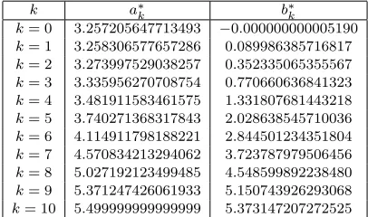
We solve the corresponding discrete time optimization problem (2.14) for this problem, by assumptionN = 10 and by using FMINCON function in Matlab software. The approximate solutionsa∗k andb∗k fork= 0,1,2, . . . , N are given in Table1. In Table
Table 1. The coefficientsa∗k andbk∗,fork= 0,1, . . . ,10 in Example 3.1.
k a∗k b∗k
k= 0 3.257205647713493 −0.000000000005190
k= 1 3.258306577657286 0.089986385716817
k= 2 3.273997529038257 0.352335065355567
k= 3 3.335956270708754 0.770660636841323
k= 4 3.481911583461575 1.331807681443218
k= 5 3.740271368317843 2.028638545710036
k= 6 4.114911798188221 2.844501234351804
k= 7 4.570834213294062 3.723787979506456
k= 8 5.027192123499485 4.548599892238480
k= 9 5.371247426061933 5.150743926293068
k= 10 5.499999999999999 5.373147207272525
Table 2. The values ofy(t) fort= 0,0.1, . . . ,1 in Example 3.1.
t Approximate solution Exact solution 0.0 3.257205647713493 3.257205647717832 0.1 3.275623816473727 3.275623816476181 0.2 3.331321581289175 3.331321581291895 0.3 3.425641420573009 3.425641420564865 0.4 3.560863537311638 3.560863537324633 0.5 3.740271368317845 3.740271368319426 0.6 3.968246145139263 3.968246145128546 0.7 4.250393467673129 4.250393467685512 0.8 4.593705860687058 4.593705860688228 0.9 5.006766424282846 5.006766424282001 1.0 5.499999999999999 5.500000000000000
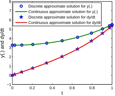
it can be seen in this table, the obtained values are very near to the exact values. Also, the graphs of discrete and continuous approximate solutions for y(·) and y′(·) are presented in Figure 1. The absolute error of the presented method, i.e. the absolute difference between the approximate solution and the analytical solution, is compared with other numerical methods in Table3. The numerical methods selected for comparison are the higher order finite difference method (HFDM) [19], the cubic B-spline method (CBSM) [7], the quartic B-spline method (QBSM) [14] and the modified cubic B-spline method (MCBSM) [34]. As one clearly observes, the absolute error of our method is less than those of the other ones and therefore by the proposed method we can obtain a better approximate solution for this SBVP. The absolute error of our proposed method for different values ofN, is given in Figure 2 which shows that when we increase the number of nodes, i.e. N, the absolute error tends to zero.
Example 3.2. Consider the following singular second-order boundary value problem
y′′(t) +1
ty
′(t) = ( 8
8−t2) 2,
Figure 1. Discrete and continuous approximate solutionsy(.) and y′(.) in Example 3.1.
0 0.2 0.4 0.6 0.8 1
−1 0 1 2 3 4 5 6 7 8
t
y(.) and dy/dt
Discrete approximate solution for y(.) Continuous approximate solution for y(.) Discrete approximate solution for dy/dt Continuous approximate solution for dy/dt
Figure 2. Absolute error of our method for Example 3.1.
0 0.2 0.4 0.6 0.8 1
0 1 2 3 4
x 10−13
t
Absolute error
N=12 N=14 N=16
Table 3. Comparison of absolute error for Example 3.1.
t Our method for
N= 10
HFDM [19] for
N= 20
CBSM [7] for
N= 20
QBSM [14] for
N= 20
MCBSM [34] forN= 20 0.0 4.3×10⁻¹² 6.16×10⁻⁷ 2.97×10⁻⁴ 5.26×10⁻⁸ 9.23×10⁻⁶
0.1 2.4×10⁻¹² 6.13×10⁻⁷ 2.95×10⁻⁴ 5.26×10⁻⁸ 3.84×10⁻⁷
0.2 2.7×10⁻¹² 6.03×10⁻⁷ 2.92×10⁻⁴ 5.25×10⁻⁸ 1.73×10⁻⁷
0.3 8.1×10⁻¹² 5.58×10⁻⁷ 2.85×10⁻⁴ 5.21×10⁻⁸ 1.05×10⁻⁷
0.4 1.3×10⁻¹¹ 5.54×10⁻⁷ 2.75×10⁻⁴ 5.12×10⁻⁸ 7.19×10⁻⁸
0.5 1.5×10⁻¹² 5.14×10⁻⁷ 2.58×10⁻⁴ 4.94×10⁻⁸ 5.24×10⁻⁸
0.6 1.1×10⁻¹¹ 4.59×10⁻⁷ 2.36×10⁻⁴ 4.62×10⁻⁸ 3.89×10⁻⁸
0.7 1.3×10⁻¹¹ 3.85×10⁻⁷ 2.02×10⁻⁴ 4.08×10⁻⁸ 2.83×10⁻⁸
0.8 1.1×10⁻¹² 2.89×10⁻⁷ 1.54×10⁻⁴ 3.22×10⁻⁸ 1.88×10⁻⁸
0.9 0.8×10⁻¹² 1.63×10⁻⁷ 8.96×10⁻⁴ 1.92×10⁻⁸ 9.62×10⁻⁹
Table 4. The coefficientsa∗k andbk∗,fork= 0,1, . . . ,10 in Example 3.2.
k a∗k b∗k
k= 0 −0.267062785263904 −0.000000000011761
k= 1 −0.264561221454872 0.050062578414913
k= 2 −0.257037701610039 0.100502512383910
k= 3 −0.244435265441268 0.151706700500273
k= 4 −0.226657370635746 0.204081632707703
k= 5 −0.203565388624767 0.258064515999351
k= 6 −0.174974908232746 0.314136125706599
k= 7 −0.140650633462087 0.372836218429264
k= 8 −0.100299567373873 0.434782608635710
k= 9 −0.053562045354685 0.500695410324417
k= 10 −0.000000000000000 0.571428571428639
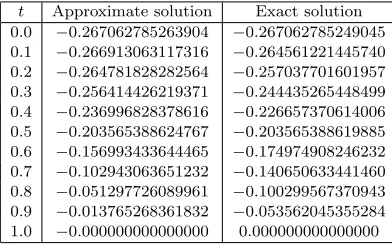
Table 5. The values ofy(t) fort= 0,0.1, . . . ,1 in Example 3.2.
t Approximate solution Exact solution 0.0 −0.267062785263904 −0.267062785249045 0.1 −0.266913063117316 −0.264561221445740 0.2 −0.264781828282564 −0.257037701601957 0.3 −0.256414426219371 −0.244435265448499 0.4 −0.236996828378616 −0.226657370614006 0.5 −0.203565388624767 −0.203565388619885 0.6 −0.156993433644465 −0.174974908246232 0.7 −0.102943063651232 −0.140650633441460 0.8 −0.051297726089961 −0.100299567370943 0.9 −0.013765268361832 −0.053562045355284 1.0 −0.000000000000000 0.000000000000000
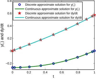
Figure 3. Discrete and continuous approximate solutionsy(.) and y′(.) in Example 3.2.
0 0.2 0.4 0.6 0.8 1
−0.2 0 0.2 0.4 0.6 0.8
t
y(.) and dy/dt
Discrete approximate solution for y(.) Continuous approximate solution for y(.) Discrete approximate solution for dy/dt Continuous approximate solution for dy/dt
Figure 4. Absolute error of our method for Example 3.2.
0 0.2 0.4 0.6 0.8 1
0 1 2 3 4 5
x 10−13
t
Absolute error
N=12 N=14 N=16
Example 3.3. Consider the following singular boundary value problem
y′′(t) +1
ty
′(t) =−ey(t),
y′(0) = 0, y(1) = 0.
The exact solution of this problem isy(t) = 2 ln( 4−2√2
(3−2√2)x2+1). The discrete approx-imate solutionsak∗ and b∗k forN = 10 and k = 0,1,2, . . . , N are given in Table 7.
Table 6. Comparison of absolute error for Example 3.2.
t Our method
forN= 10
HFDM [19] forN= 20
CBSM [8] for
N= 20
QBSM [14] forN= 20
MCBSM [34] forN= 20 0.0 1.5×10⁻¹¹ 9.22×10⁻⁵ 2.72×10⁻⁵ 9.40×10⁻⁹ 2.57×10⁻⁸
0.1 9.1×10⁻¹² 9.04×10⁻⁵ 2.69×10⁻⁵ 9.29×10⁻⁹ 1.52×10⁻⁸
0.2 8.1×10⁻¹² 8.61×10⁻⁵ 2.63×10⁻⁵ 9.15×10⁻⁹ 1.08×10⁻⁸
0.3 7.2×10⁻¹² 8.15×10⁻⁵ 2.53×10⁻⁵ 8.92×10⁻⁹ 8.13×10⁻⁹
0.4 2.7×10⁻¹¹ 7.68×10⁻⁵ 2.38×10⁻⁵ 8.56×10⁻⁹ 6.23×10⁻⁹
0.5 4.9×10⁻¹² 7.17×10⁻⁵ 2.18×10⁻⁵ 8.05×10⁻⁹ 4.74×10⁻⁹
0.6 1.3×10⁻¹¹ 6.61×10⁻⁵ 1.92×10⁻⁵ 7.31×10⁻⁹ 3.49×10⁻⁹
0.7 2.1×10⁻¹¹ 5.92×10⁻⁵ 1.59×10⁻⁵ 6.28×10⁻⁹ 2.43×10⁻⁹
0.8 1.1×10⁻¹² 4.97×10⁻⁵ 1.17×10⁻⁵ 4.85×10⁻⁹ 1.50×10⁻⁹
0.9 6.0×10⁻¹³ 3.43×10⁻⁵ 6.51×10⁻⁶ 2.83×10⁻⁹ 6.92×10⁻¹⁰
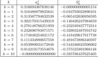
Table 7. The coefficientsa∗k andbk∗,fork= 0,1, . . . ,10 in Example 3.3.
k a∗k b∗k
k= 0 0.316694367638146 −0.000000000005154
k= 1 0.316488879825641 −0.016793022896101
k= 2 0.313567794632539 −0.065432636956595
k= 3 0.302170315439319 −0.140426247984659
k= 4 0.276148766251959 −0.232349437772314
k= 5 0.232696783871571 −0.329032487934742
k= 6 0.174848254821172 −0.418429617917738
k= 7 0.111334880657558 −0.491673886340597
k= 8 0.053989034172848 −0.544346623506062
k= 9 0.014210173554678 −0.575525891968148
k= 10 −0.000000000000000 −0.585786437625405
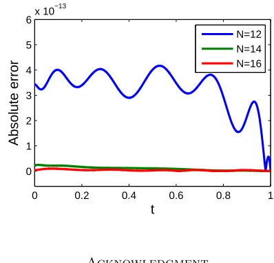
exact values are presented in Table 8. In Figure5, the discrete and continuous ap-proximate solutions fory(·) andy′(·) are shown. The absolute error of the proposed method is compared with those of two other numerical methods [21,27] in Table 9. We can see that, the absolute error of the proposed method is less than those of the other ones and therefore by our method we can obtain a better approximate solution for this SBVP. The absolute error of our proposed method for different values ofN
is given in Figure6.
4. Conclusions
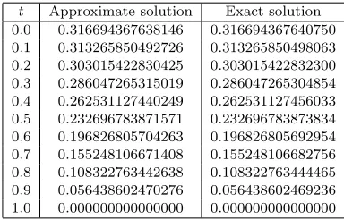
Table 8. The values ofy(t) fort= 0,0.1, . . . ,1 in Example 3.3.
t Approximate solution Exact solution 0.0 0.316694367638146 0.316694367640750 0.1 0.313265850492726 0.313265850498063 0.2 0.303015422830425 0.303015422832300 0.3 0.286047265315019 0.286047265304854 0.4 0.262531127440249 0.262531127456033 0.5 0.232696783871571 0.232696783873834 0.6 0.196826805704263 0.196826805692954 0.7 0.155248106671408 0.155248106682756 0.8 0.108322763442638 0.108322763444465 0.9 0.056438602470276 0.056438602469236 1.0 0.000000000000000 0.000000000000000
Figure 5. Discrete and continuous approximate solutionsy(.) and
y′(.) in Example 3.3.
0 0.2 0.4 0.6 0.8 1
−0.6 −0.4 −0.2 0 0.2 0.4 0.6 0.8
t
y(.) and dy/dt
Discrete approximate solution for y(.) Continuous approximate solution for y(.) Discrete approximate solution for dy/dt Continuous approximate solution for dy/dt
Table 9. Comparison of absolute error of Example 3.3.
t Our method for
N= 10
Approach in [21] forN= 20
Approach in [27] forN= 10
Approach in [27] forN= 14 0.0 2.6×10⁻¹² 2.00×10⁻⁶ 3.77×10⁻⁸ 6.72×10⁻⁸
0.1 5.3×10⁻¹² 1.99×10⁻⁶ 1.05×10⁻⁷ 6.69×10⁻⁸
0.2 1.8×10⁻¹² 1.97×10⁻⁶ 6.33×10⁻⁹ 7.87×10⁻⁹
0.3 1.0×10⁻¹² 1.94×10⁻⁶ 5.91×10⁻⁸ 6.92×10⁻⁹
0.4 1.5×10⁻¹¹ 1.83×10⁻⁶ 2.12×10⁻⁷ 2.87×10⁻⁸
0.5 2.2×10⁻¹² 1.78×10⁻⁶ 1.00×10⁻⁸ 7.40×10⁻¹⁰
0.6 1.1×10⁻¹¹ 1.67×10⁻⁶ 5.36×10⁻⁷ 6.32×10⁻⁸
0.7 1.1×10⁻¹¹ 1.34×10⁻⁶ 4.25×10⁻⁸ 6.95×10⁻⁸
0.8 1.8×10⁻¹² 9.20×10⁻⁷ 8.32×10⁻⁷ 3.38×10⁻⁹
Figure 6. Absolute error of our method for Example 3.3.
0 0.2 0.4 0.6 0.8 1
0 1 2 3 4 5 6x 10
−13
t
Absolute error
N=12 N=14 N=16
Acknowledgment
The authors would like to express their heartfelt thanks to the editor and anony-mous referees for their useful suggestions which improved the quality of the paper.
References
[1] J. A. Adam,A simplified mathematical model of tumor growth, Math. Biosci.,81(1986), 224– 229.
[2] J. A. Adam,A mathematical model of tumor growth II: effect of geometry and spatial
non-uniformity on stability, Math. Biosci.,86(1987), 183–211.
[3] J. A. Adam and S. A. Maggelakis,Mathematical model of tumor growth IV: effect of necrotic core, Math. Biosci.,97(1989), 121–136.
[4] N. S. Asaithambi and J. B. Goodman, Point wise bounds for a class of singular diffusion
problems in physiology, Appl. Math. Comput.,30(1989), 215-222.
[5] D. Benko, D. C. Biles, M. P. Robinson, and J. S. Spraker, Nystrom methods and singular
second-order differential equations, Computers & Mathematics with Applications,55(8) (2008),
1975–1980.
[6] A. C. Burton, Rate of growth of solid tumor as a problem of diffusion, Growth, 30 (1966), 157–176.
[7] N. Caglar and H. Caglar,B-spline solution of singular boundary value problems, Appl. Math. Comput.,182(2006), 1509–1513.
[8] H. Caglar, N. Caglar, and M. Ozer, B-spline solution of non-linear singular boundary value
problems arising in physiology, Chaos, Solitons and Fractals,39(3) (2009), 1232–1237.
[9] M. G. Cui and F. Z. Geng,Solving singular two-point boundary value problem in reproducing
kernel space, J. Comput. Appl. Math.,205(2007), 6–15.
[10] F. Fahroo and I. M. Ross,Direct trajectory optimization by a Chebyshev pseudospectral method, Journal of Guidance, Control and Dynamics,25(1) (2002), 160–166.
[11] F. Fahroo and I. M. Ross,Costate estimation by a legendre pseudospectral method, Journal of Guidance, Control, and Dynamics,24(2) (2001), 270–277.
[13] M. Ghaznavi and M. H. Noori Skandari, An efficient pseudo-spectral method for
non-smooth dynamical systems, Iran. J. Sci. Technol. Trans. Sci, (2016), In press. DOI
https://doi.org/10.1007/s40995-016-0040-9.
[14] J. Goh, A. Majid, and A. I. Ismail,A quartic B-spline for second-order singular boundary value
problems, Comput. Math. Appl.,64(2012), 115–120.
[15] B. F. Gray,The distribution of heat sources in the human head: theoretical considerations, J. Theor. Biol.,82(1980), 473–476.
[16] M. K. Kadalbajoo and V. K. Aggarwal,Numerical solution of singular boundary value problems
via Chebyshev polynomial and B-spline, Appl. Math. Comput.,160(2005), 851–863.
[17] A. S. V. R. Kanth,Cubic spline polynomial for non-linear singular two-point boundary value
problems, Appl. Math. Comput.,189(2007), 2017–2022.
[18] A. S. V. R. Kanth and V. Bhattacharya,Cubic spline for a class of non-linear singular boundary
value problems arising in physiology, Appl. Math. Comput.,174(1) (2006), 768–774.
[19] A. S. V. R. Kanth and Y. N. Reddy,Higher order finite difference method for a class of singular
boundary value problems, Appl. Math. Comput.,155(2004), 249–258.
[20] A. S. V. R. Kanth and Y. N. Reddy,Cubic spline for a class of singular two-point boundary
value problems, Appl. Math. Comput.,170(2005), 733–740.
[21] S. A. Khuri and A. Sayfy,A novel approach for the solution of a class of singular boundary
value problems arising in physiology, Mathematical and Computer Modelling, 52(3-4) (2010),
626–636.
[22] M. Kumar,A difference method for singular two-point boundary value problems, Applied Math-ematics and Computation,146(2-3) (2003), 879–884.
[23] M. Kumar and Y. Gupta,Methods for solving singular boundary value problems using splines:
A review, J. Appl. Math. Comput.,32(2010), 265–278.
[24] M. Kumar and N. Singh,Modified Adomian decomposition method and computer
implementa-tion for solving singular boundary value problems arising in various physical problems,
Com-puters and Chemical Engineering,34(11) (2010), 1750–1760.
[25] H. S. Lin,Oxygen diffusion in a spherical cell with nonlinear oxygen uptake kinetics, J. Theor. Biol.,60(1976), 449–457.
[26] D. L. S. McElwain,A re-examination of oxygen diffusion in a spherical cell with
Michaelis-Menten oxygen uptake kinetics, J. Theor. Biol.,71(1978), 255-263.
[27] M. Mohsenyzadeh, K. Maleknejad, and R. Ezzati,A numerical approach for the solution of a
class of singular boundary value problems arising in physiology, Advances in Difference
Equa-tions,2015(2015), 1–10.
[28] M. H. Noori Skandari and M. Ghaznavi,Chebyshev pseudo-spectral method for Bratu’s problem, Iran. J. Sci. Technol. Trans. Sci, (2015), In press. DOI 10.22099/IJSTS.2015.3473.
[29] M. H. Noori Skandari, A. V. Kamyad, and S. Effati,Generalized Euler-Lagrange equation for
nonsmooth calculus of variations, Nonlinear Dynamics,75(1-2) (2014), 85–100.
[30] M. H. Noori Skandari, A. V. Kamyad, and S Effati,Smoothing approach for a class of nonsmooth
optimal control problems, Applied Mathematical Modelling,40(2) (2016), 886–903.
[31] W. Y. Wang, M. G. Cui, and B. Han,A new method for solving a class of singular two-point
boundary value problems, Appl. Math. Comput.,206(2008), 721–727.
[32] A. M. Wazwaz,The variational iteration method for solving nonlinear singular boundary value
problems arising in various physical models, Communications in Nonlinear Science and
Numer-ical Simulation,16(10) (2011), 3881–3886.
[33] A. Yildirim and T. Ozis, Solutions of singular IVPs of Lane-Emden type by the variational
iteration method, Nonlinear Analysis: Theory, Methods and Applications,70(6) (2009), 2480–
2484.