Abstract— In this paper an approach to apply inventory decisions in facility location problem is presented. In fact, there are many models which are concerned with some of the inventory decisions in distribution network design and most of them shortly utilize inventory elements. The contribution is to minimize total establishment, transportation and inventory costs in a multi-commodity single-period distribution system and is supported by a case study to be implemented and the solutions are followed. The demand of customer is assumed to be deterministic.
Index Terms— Distribution System, Facility location, Inventory, Multi-Objective, Single-Period.
I. INTRODUCTION
Increasing global competition and merging big companies, especially vertical integration, have caused corporations to control their costs more than ever while simultaneously optimizing the facility locations and paying more attentions to their customers’ needs. So that’s why reviewing concepts and innovations in mentioned areas look to be essential.
Supply chain management is an integrative approach to manage material and information flows with suppliers and customers as well as between different functions within a company. Distribution system too as a part of supply chain philosophy, seeks the same purpose from focal company to customers. According to the comprehensive concepts of supply chain management, many sciences, interdisciplinary fields and techniques are applied in to support the whole chain by optimize decisions like inventory decisions, capacity planning, procurement, routing, transportation mode, etc.
In spite of the need to integrate SC components into a single SC and despite the limited progress made towards doing this, most studies on SC design and optimization focus on a single component of the overall system (e.g. procurement, production, transportation, inventory management, etc.) [11]. only a few studies propose useful operational models and methods enabling managers and practitioners to optimize SCs by focusing on the effectiveness of the whole system, i.e. by determining a global optimum.
As describe by [9], the generic facility location problem in logistic systems is defined by taking simultaneous decisions regarding design, management and control of generic
All Authors are with Industrial Engineering Department of Amirkabir University of Technology(AUT), 424 Hafez Ave., Tehran, Iran (corresponding author to provide phone: +989153138065; e-mail: h.afshari@ aut.ac.ir).
distribution network ([1],[4],[13],[14],[16],[22]).
[15] Presented a review of the literature on facility location and supply chain management. The abstract of mentioned papers in facility location are:
1. Location of new supply facilities in a given set of demand points. The demand points correspond to existing customer locations.
2. Demand flows to be allocated to available or new suppliers (i.e. production and/or distribution facilities).
3. Configuration of a transportation network, i.e. design of paths from suppliers to customers, management of routes and vehicles in order to supply demand needs simultaneously.
In fact facility location problem, in many papers and researches, is introduced as strongly associating with effective management of multi-stage production and distribution networks. Many papers in recent years have studied the facility location ([3],[10],[13],[14],[23],[27],[28]) and all of them have brought contributions to the main concept.
Before trying to consolidate different components with facility location problem, it’s necessary to review all types of decisions in supply chain management and assess that how is it possible to join them with facility location problem. The decisions making and planning in supply chain management are divided into 3 main categories[14]:
• Strategic planning, which is related to long-term
planning horizon(e.g.3–5years) and to the strategic problem of designing and configuring a generic multi- stage SC. Management decisions deal with the determination of the number of facilities, geographical locations, capacity of facilities, and allocation of customer demand [13].
• Tactical planning, This level refers to both long-and
short-term planning horizons and deals with the determination of the best fulfillment policies and material flows in an SC, modeled as a multi-echelon inventory distribution system [14].
• Operational planning, The variable time is introduced, correlating the determination of the number of logistic facilities, geographical locations, facilities capacity to the optimal daily allocation of customer demand, to retailers, DCs, and/or production plants.
Inventory decisions usually are categorized as operational and tactical level of planning. But by organizing available long-term information in single-period problems, it’s possible to use this information in strategic planning and therefore, inventory and facility location could be joined for strategic planning.
[7],[12],[13],[14],[15],[23] presented some classification
Optimizing Inventory Decisions in Facility
Location within Distribution Network Design
on the main general classes of effective and quantitative methods for facility location and location and allocation problem.
The joint location-inventory management problem was first examined in simplified linear version by [2] and [25]. [24] Proposed a mixed-integer linear model for the design and planning of a production–distribution system.
[6] and [8] proposed approaches to solve non-linear models which concerns simultaneously distribution network design and inventory optimization.
Multi-stage version of the joint location-inventory management problem was optimally solved by [5], [19], and [20]. [5] Proposed a lagrangian relaxation solution algorithm for the case in which the ratio of the variance to the mean of the demand is identical for all customers. [19] Continued the method suggested by [5] by presenting non-linear integer set-covering models that also perform well with deterministic demand (that is when the ratio of the variance to the mean of the demand is equal to 0 for all customers). [20] Studied on the general version of the problem (that is, when the ratio of the variance to the mean of the demand is not identical for all customers). Further aspects with practical relevance have also recently been added to the aforementioned pioneer approaches. [20] Presented a set-partitioning integer programming model to determine the optimal inventory replenishment strategy for both DCs and retailers. [17] Proposed an analytical model for coupling location-inventory management with capacity constraints and congestion costs, which occurs when DCs operate quite near their saturation condition. [19] Introduced a vehicle routing model for optimizing products shipping between DCs and customer points of demands. [22] Formulated the stochastic version of the joint location-inventory management problem, by introducing the likelihood of occurrence of each cost factor into the objective function. Nevertheless, the aforementioned papers do not simultaneously optimize production and distribution activities in conditions of uncertainty nor do they assume a non-linear dynamic perspective. [9] Proposed a non-linear model supporting strategic, tactical, and operational choices of decision-makers in the field of facility location, inventory, and production management is formulated in a multi-period perspective.
The study conducted by authors contains an optimization of location-inventory management in multi-stage, multi-commodity network design problem. For more explanation and comparison, a literature review is illustrated in Table1.
II. MODEL DESCRIPTION
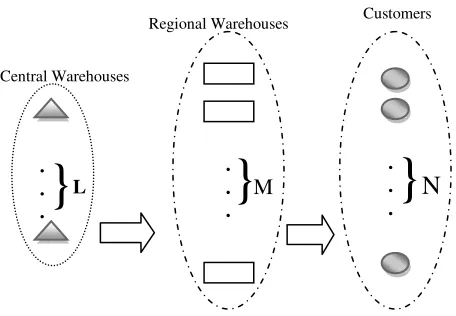
Components of supply chain such as are illustrated in Figure 1 are introduced.
Central warehouses: the main stocks of supply chain that demands are supplied here. There are L potential location for central warehouses, capital of country and south port.
Regional warehouses: stocks between central warehouses and customers that demands are distributed here. There are M potential locations for regional warehouses that they are in the capital of provinces.
Customers: there are N customers that are located in the cities of the provinces.
Goods: O types of commodities can be supplied for the
customers demanding O families of cars. Assumptions of problem are as follows:
• There are L potential central warehouses that at
least one of them should be located,
• There are limited capacities for both central and
regional warehouses.
• Transportation cost per unit is as a coefficient of distance between central and regional warehouses and between regional warehouses and customers. The objective for supply chain is minimizing total cost including establishment and transportation cost.
Fig 1. Components of supply chain
III. MODEL FORMULATION A. Sets and indices
Sets of central warehouses || , , Sets of regional warehouses || , , Sets of customers || , ,
Sets of good types|| , . B. Variables
1, If the potential point of for central warehouses is located,
0, Otherwise, +
,- regional warehouses is located,1, If the potential point of for 0, Otherwise,
+
/0-1 Percentage of demand customer for commodity that is supplied by regional warehouse,
2-1 Percentage of demand regional warehouse for commodity that is supplied by central warehouse. C. Parameters
301 Demand of customer for commodity,
4-1 Capacity of regional warehouse for commodity , 5 Cost of transportation per unit,
60- Distance between regional warehouse and customer ,
6-7 Distance between regional warehouse and central warehouse ,
81 Capacity of central warehouse for commodity , 9 Cost of installation central warehouse ,
:01 Minimum level of customer satisfaction for commodity .
;- Cost of installation regional warehouse , <= Warehousing cost per unit goods in warehouses <> Warehousing cost per unit goods in stocks ? Back ordered cost per unit goods
M
N
Customers
Central Warehouses
Regional Warehouses
. .
.
}
L
}
. . .
. .
.
}
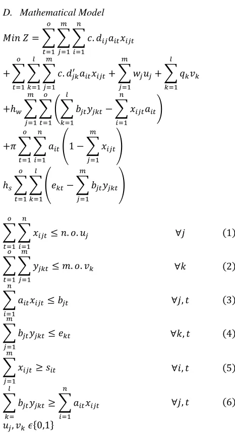
[image:2.595.305.533.208.366.2]D. Mathematical Model
@ A A A 5. 60-301/0-1
C
0DE F
-DE G
1DE
H A A A 5. 6-7 301/0-1 F
-DE I
DE G
1DE
H A ; -,-F
-DE
H A 9 I
DE
H<=A A JA 4-12-1 I
DE
K A /0-1301 C
0DE
L G
1DE F
-DE
H? A A 301M1 K A /0-1 F
-DE N C
0DE G
1DE
<>A A M81K A 4-12-1 F
-DE
N I
DE G
1DE
A A /0-1 C
0DE G
1DE
O . . ,- P 1
A A 2-1 F
-DE G
1DE
O . . P 2
A 301/0-1 C
0DE
O 4-1 P, 3
A 4-12-1 F
-DE
O 81 P, 4
A /0-1 F
-DE
T :01 P, 5
A 4-12-1 I
D
T A 301/0-1 C
0DE
P, 6
,-, W0,1X
Objective function @ is summation of:
• Transportation cost between central and regional warehouses, ∑ ∑ ∑ 5. 6G1DE F-DE C0DE 0-301/0-1,
• Transportation cost between regional warehouses and customer, ∑ ∑G1DE IDE∑ 5. 6F-DE -7 301/0-1,
• Installation cost for central
warehouses, ∑ ;F-DE -,- and
• Installation cost for regional warehouses,∑IDE9, that is multiplied by weighted coefficient Z.
Constraints (1) and (2) states if regional warehouse or central warehouse satisfy the demand, it has been installed. Constraints (3) and (4) show capacity restriction for each regional warehouse. Constraint (5) implies that there is a minimum level of customer satisfaction for commodity . Constraint (6) considers that amount of supply should be greater than amount of demand.
IV. COMPUTATIONAL RESULTS A. Case study
This model was presented for a practical case in Automotive Part Distribution Corporation which was extended to be replaced with previous one. Former distribution system contained one central warehouse and the commodities were directly transshipped to customers. This outmoded distribution system was faced with new aggravating problems and management board decided to apply new distribution system.
To improve these indexes, new distribution system was applied to be adjacent to customer zone and agile response to customer needs and to increase market share. Therefore all of the customers were categorized to particular zones in order to create nominated areas for establishing regional warehouses. The assumptions for studied are described as below:
• The number of goods is 5,
• The number of candidate central warehouses is 2, • The number of candidate regional warehouses is 8
and,
• The number of candidate customer is 28.
[image:3.595.44.277.44.473.2]The parameters and constants which are used in this model are gained based on real data of system and eagerly chased to see the model outcomes. So for comparison, some criteria are considered to assess the efficiency of model.
Table 1. Literature review of common inventory-facility location models
Authors year
Model Costs
Number of stages
Production plants
Central Depots
Regional Depots
Customers Products* Multi-Period
Production transportation Warehousing Inventory Stockout
Authors
approach - 2 - Yes Yes Yes MP - - Yes Yes Yes Yes Gebennini et
al 2009 2 Yes - Yes Yes SP Yes Yes Yes Yes Yes Yes Miranda et al. 2009 2 Yes - Yes Yes SP - Yes Yes Yes Yes -
Thanh et al. 2008 3 Yes - Yes Yes MP Yes Yes Yes Yes Yes - Tsiakis and
Papageorgiou 2008 2 Yes - Yes Yes MP - Yes Yes Yes Yes - Snyder et al. 2007 2 Yes - Yes Yes SP Yes - Yes Yes Yes - Shen and Qi 2007 2 Yes - Yes Yes SP - - Yes Yes Yes - Romeijn et al. 2007 2 Yes - Yes Yes SP - - Yes Yes Yes - Shu et al. 2005 2 Yes - Yes Yes SP - - Yes Yes Yes - Ambrosino
and Scutella 2005 3 Yes Yes Yes Yes SP Yes - Yes Yes Yes - Teo and Shu 2004 2 Yes - Yes Yes SP - - Yes Yes Yes - Shen et al. 2003 2 Yes - Yes Yes SP - - Yes Yes Yes - Freling et al. 2003 1 Yes - - Yes SP Yes - Yes - Yes - Daskin et al. 2002 2 Yes - Yes Yes SP - - Yes Yes Yes -
Erlenbacher
B. Experimental results
As designed and considered in the model, this can be applied for many real cases and because of the multi-commodity nature of the model, the satisfaction index and other factors could be measured based on goods type.
Another factor which can drastically support the managers is the minimum satisfaction level which the computation results of the model is shown at different
:
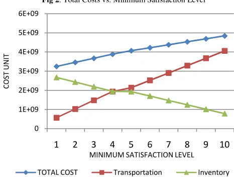
01 in Table 2. For example, the Fig 2 demonstrates the objective function value in different minimum customer satisfaction values.Fig 2. Total Costs vs. Minimum Satisfaction Level
As Inventory costs is highlighted in this paper, total warehousing and shortage costs are illustrated in Fig2 to analyze the effects on satisfaction level.
According to Fig 3 the inventory costs decrease as customer satisfaction increase. It could be interpreted by lower costs which are related to the shortage because of higher availability rate in regional warehouses. The other supporting reason is this that as customer satisfaction increases, more goods would be sent to customers so the warehousing costs in central and regional warehouses will be decreased.
Fig 3. Inventory Costs vs. Customer Satisfaction
[image:4.595.41.569.56.157.2]According to Fig 2, the minimum satisfaction level at 40% which creates 46% total customer satisfaction is the point that approximately inventory costs and transportation cost are equal. It means before minimum satisfaction level, it is better to send the goods directly to the customers. Based on the desired satisfaction level, the managers could decide about the number and the place of central and regional warehouses. Table 3 demonstrates calculation results of model for mentioned case studied at :01=0.4 and :01=1.
Table 3. Results of designed model at :01 =0.4 and :01=1
Variable Title Value
Total Cost([\) 4.56E+09
4.84E+09
Customer
Satisfaction 46% 100%
]
^_ 0.4 1V(1,2) (1,1)
U(1,2,3,4,5,6,7,8) (0,0,0,0,0,0,0,1) (0,0,0,0,0,1,0,1)
V. CONCLUSION
Inventory management is one of the important concerns which are highly considerable by management nowadays. In distribution network design, it could be shown as inventory costs and includes warehousing, inventory and stock out costs.
In this paper a mixed integer programming model, which is solved with LINGO software, is presented to coup with the facility location problem in multi-commodity, single period problem with inventory concerns. The model is used for a case study in automobile parts distribution network design.
The results are used to find locations for central and regional warehouses. Also the results showed to be practical and useful because of great similarities between the model and the studies case and ensured that this model can be applied for other cases.
Finally, the future extensions to the model could be consideration of the multi-stage situation. Another suggestion is to add components to fulfill demand uncertainties.
REFERENCES
[1] Agatz, N.A.H., Fleischmann,M., van NunenJo, A.E.E., 2008. E-fulfillment and multi-channel distribution—a review. European Journal of Operational Research 187, 339–356.
[2] Ambrosino, D., Scutella`, M.G., 2005. Distribution network design: new problems and related models. European Journal of Operational Research 165, 610–624.
[3] Baker,P., 2008. The design and operation of distribution centers within agile supply chains. International Journal of Production Economics 111, 27–41.
0 1E+09 2E+09 3E+09 4E+09 5E+09 6E+09
1 2 3 4 5 6 7 8 9 10
C
O
S
T
U
N
IT
MINIMUM SATISFACTION LEVEL
TOTAL COST Transportation Inventory
0.0E+00 5.0E+08 1.0E+09 1.5E+09 2.0E+09 2.5E+09 3.0E+09
0.20 0.29 0.38 0.46 0.57 0.67 0.75 0.83 0.92 1.00
IN
V
E
N
T
O
R
Y
C
O
S
T
S
CUSTOMER SATISFACTION
Table 2. Results of designed model at different :01
Minimum Satisfaction Level
0.1 0.2 0.3 0.4 0.5 0.6 0.7 0.8 0.9 1
Objective Fun. Value 3.25E+09 3.46E+09 3.67E+09 3.88E+09 4.07E+09 4.22E+09 4.38E+09 4.53E+09 4.69E+09 4.84E+09
Total Satisfaction 0.20 0.29 0.38 0.46 0.57 0.67 0.75 0.83 0.92 1.00
Total Transportation
Cost 5.71E+08 1.03E+09 1.48E+09 1.94E+09 2.14E+09 2.52E+09 2.91E+09 3.29E+09 3.68E+09 4.06E+09
[image:4.595.309.543.311.399.2] [image:4.595.50.283.313.489.2] [image:4.595.48.268.663.770.2][4] Chen, I.J., Paulraj,A., 2004. Understanding supply chain management: critical research and a theoretical framework. International Journal of Production Research 42, 131–163.
[5] Daskin, M., Coullard, C., Shen, Z.J., 2002. An inventory-location model: formulation, solution algorithm and computational results. Annals of Operations Research 110, 83–106.
[6] Erlebacher,S.J., Meller,R.D., 2000. The interaction of location and inventory in designing distribution systems. IIE Transactions 32, 155– 166.
[7] Francis, R.L., McGinnis, L.F., White, J.A., 1992. Facility Layout and Location. Prentice-Hall, New Jersey.
[8] Freling, R., Romeijn, H.E., Morales, D.R., Wagelmans, A.P.M., 2003. A branch-and-price algorithm for multi period single-sourcing problem. Operations Research 51, 922–939.
[9] Gebennini, E, Gamberini, R, Manzini, R, 2009. An integrated production–distribution model for the dynamic location and allocation problem with safety stock optimization. International Journal of Production Economics 122, 286–304
[10] Hinojosa, Y., Kalcsics, J., Nickel, S., Puerto, J., Velten, S., 2008. Dynamic supply chain design with inventory. Computers & Operations Research 35, 373–391.
[11] Liang, T.-F., 2008. Integrating production–transportation planning decision with fuzzy multiple goals in supply chains. International Journal of Production Research 46, 1477–1494.
[12] Love, R.F., Morris, J.G., Wesolowsky, G.O., 1988. Facilities Location. Models & Methods. North-Holland, New York.
[13] Manzini, R., Gamberi, M., Regattieri,A.,2006. Applying mixed integer programming to the design of a distribution logistic network. International Journal of Industrial Engineering: Theory Applications and Practice 13(2),207–218.
[14] Manzini, R., Gebennini, E., 2008. Optimization models for the dynamic facility location and allocation problem. International Journal of Production Research 46(8), 2061–2086.
[15] Melo, M.T., Nickel, S., Saldanha-da-Gama,F.,2009. Facility location and supply chain management—a review .European Journal of Operational Research 196,401–412.
[16] ReVelle, C.S., Eiselt, H.A., Daskin, M.S., 2008. A bibliography for some fundamental problem categories in discrete location science. European Journal of Operational Research 184, 817–848.
[17] Romeijn, H.E., Shu, J., Teo, C.P., 2007. Designing two-echelon supply networks. European Journal of Operational Research 178, 449–462.
[18] Shen, Z.J., Coullard, C., Daskin, M., 2003. A joint location-inventory model. Transportation Science 37, 40–55.
[19] Shen, Z.J., Qi, L., 2007. Incorporating inventory and routing costs in strategic location models. European Journal of Operational Research 179, 372–389.
[20] Shu, J., Teo, C.P., Shen, Z.J., 2005. Stochastic transportation-inventory network design problem. Operations Research 53, 48–60. [21] Snyder, L.V., 2006. Facility location under uncertainty: a review. IIE
Transactions 38, 537–554.
[22] Snyder, L.V., Daskin, M., Teo, C.P., 2007. The stochastic location model with risk pooling. European Journal of Operational Research 179, 1221–1238.
[23] Sule, D.R., 2001. Logistics of Facility Location and Allocation. Marcel Dekker Inc., New York.
[24] Thanh, P.N., Bostel, N., Peton, O., 2008. A dynamic model for facility location in the design of complex supply chains. International Journal of Production Economics 113, 678–693.
[25] Tsiakis, P., Papageorgiou, L.G., 2008. Optimal production allocation and distribution supply chain networks. International Journal of Production Economics 111(2), 468–483.
[26] Van der Vaart, T.,vanDonk, D.P.,2008. Acritical review of survey-based research in supply chain integration. International Journal of Production Economics 111, 42–55.
[27] Wadhwa, S., Saxena, A., Chan, F.T.S., 2008. Framework for flexibility in dynamic supply chain management. International Journal of Production research 46, 1373–1404.