A Fast Algorithm for Feature Selection in Conditional
Maximum Entropy Modeling
Yaqian Zhou
Computer Science Department
Fudan University
Shanghai 200433, P.R. China
[email protected]
Fuliang Weng
Research and Technology Center
Robert Bosch Corp.
Palo Alto, CA 94304, USA
[email protected]
Lide Wu
Computer Science Department
Fudan University
Shanghai 200433, P.R. China
[email protected]
Hauke Schmidt
Research and Technology Center
Robert Bosch Corp.
Palo Alto, CA 94304, USA
[email protected]
Abstract
This paper describes a fast algorithm that se-lects features for conditional maximum en-tropy modeling. Berger et al. (1996) presents an incremental feature selection (IFS) algo-rithm, which computes the approximate gains for all candidate features at each selection stage, and is very time-consuming for any problems with large feature spaces. In this new algorithm, instead, we only compute the approximate gains for the top-ranked features based on the models obtained from previous stages. Experiments on WSJ data in Penn Treebank are conducted to show that the new algorithm greatly speeds up the feature selec-tion process while maintaining the same qual-ity of selected features. One variant of this new algorithm with look-ahead functionality is also tested to further confirm the good quality of the selected features. The new algo-rithm is easy to implement, and given a fea-ture space of size F, it only uses O(F) more space than the original IFS algorithm.
1
Introduction
Maximum Entropy (ME) modeling has received a lot of attention in language modeling and natural language processing for the past few years (e.g., Rosenfeld, 1994; Berger et al 1996; Ratnaparkhi, 1998; Koeling, 2000). One of the main advantages
using ME modeling is the ability to incorporate various features in the same framework with a sound mathematical foundation. There are two main tasks in ME modeling: the feature selection process that chooses from a feature space a subset of good features to be included in the model; and the parameter estimation process that estimates the weighting factors for each selected feature in the exponential model. This paper is primarily con-cerned with the feature selection process in ME modeling.
While the majority of the work in ME modeling has been focusing on parameter estimation, less effort has been made in feature selection. This is partly because feature selection may not be neces-sary for certain tasks when parameter estimate al-gorithms are fast. However, when a feature space is large and complex, it is clearly advantageous to perform feature selection, which not only speeds up the probability computation and requires smaller memory size during its application, but also shortens the cycle of model selection during the training.
Feature selection is a very difficult optimization task when the feature space under investigation is large. This is because we essentially try to find a best subset from a collection of all the possible
feature subsets, which has a size of 2|W|, where |
W|
is the size of the feature space.
(Rosenfeld, 1994; Ratnaparkhi, 1998; Reynar and Ratnaparkhi, 1997; Koeling, 2000), where only the features that occur in a corpus more than a pre-defined cutoff threshold get selected. Chen and Rosenfeld (1999) experimented on a feature
selec-tion technique that uses a c2 test to see whether a
feature should be included in the ME model, where
the c2 test is computed using the count from a prior
distribution and the count from the real training data. It is a simple and probably effective tech-nique for language modeling tasks. Since ME models are optimized using their likelihood or likelihood gains as the criterion, it is important to
establish the relationship between c2 test score and
the likelihood gain, which, however, is absent. Berger et al. (1996) presented an incremental ture selection (IFS) algorithm where only one fea-ture is added at each selection and the estimated parameter values are kept for the features selected in the previous stages. While this greedy search assumption is reasonable, the speed of the IFS al-gorithm is still an issue for complex tasks. For better understanding its performance, we re-implemented the algorithm. Given a task of 600,000 training instances, it takes nearly four days to select 1000 features from a feature space with a little more than 190,000 features. Berger
and Printz (1998) proposed an f-orthogonal
condi-tion for selecting k features at the same time
with-out affecting much the quality of the selected features. While this technique is applicable for certain feature sets, such as word link features
re-ported in their paper, the f-orthogonal condition
usually does not hold if part-of-speech tags are dominantly present in a feature subset. Past work, including Ratnaparkhi (1998) and Zhou et al (2003), has shown that the IFS algorithm utilizes much fewer features than the count cutoff method, while maintaining the similar precision and recall on tasks, such as prepositional phrase attachment, text categorization and base NP chunking. This leads us to further explore the possible improve-ment on the IFS algorithm.
In section 2, we briefly review the IFS algo-rithm. Then, a fast feature selection algorithm is described in section 3. Section 4 presents a number of experiments, which show a massive speed-up and quality feature selection of the new algorithm. Finally, we conclude our discussion in section 5.
2
The Incremental Feature Selection
Al-gorithm
For better understanding of our new algorithm, we start with briefly reviewing the IFS feature selec-tion algorithm. Suppose the condiselec-tional ME model takes the following form:
†
p(
y
|
x)
=
1Z(x)
exp(
l
jf
j(x,
y))
jÂ
where fj are the features, lj are their
corre-sponding weights, and Z(x) is the normalization
factor.
The algorithm makes the approximation that the
addition of a feature f in an exponential model
af-fects only its associated weight a, leaving
un-changed the l-values associated with the other
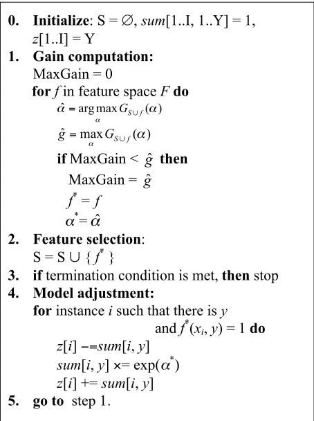
features. Here we only present a sketch of the algo-rithm in Figure 1. Please refer to the original paper for the details.
In the algorithm, we use I for the number of training instances, Y for the number of output classes, and F for the number of candidate features or the size of the candidate feature set.
0. Initialize: S = ∅, sum[1..I, 1..Y] = 1,
z[1..I] = Y
1. Gain computation:
MaxGain = 0
for f in feature space F do
) ( max arg
ˆ a
a
a S f G» =
) ( max
ˆ a
a GS f
g= »
if MaxGain < gˆ then
MaxGain = gˆ
f* = f
a*=aˆ
2. Feature selection: S = S » { f* }
3. if termination condition is met, then stop
4. Model adjustment:
for instance i such that there is y
and f*(x
i, y) = 1 do
z[i] -=sum[i, y]
sum[i, y] ¥= exp(a*)
z[i] += sum[i, y]
[image:2.612.313.540.398.702.2]5. go to step 1.
One difference here from the original IFS algo-rithm is that we adopt a technique in (Goodman, 2002) for optimizing the parameters in the
condi-tional ME training. Specifically, we use array z to
store the normalizing factors, and array sum for all
the un-normalized conditional probabilities sum[i,
y]. Thus, one only needs to modify those sum[i, y]
that satisfy f*(xi, y)=1, and to make changes to their
corresponding normalizing factors z[i]. In contrast
to what is shown in Berger et al 1996’s paper, here is how the different values in this variant of the IFS algorithm are computed.
Let us denote
Â
=
j j jf x y
x y
sum( | ) exp( l ( , ))
Â
= y x y sum xZ( ) ( | )
Then, the model can be represented by sum(y|x)
and Z(x) as follows:
) ( / ) | ( ) |
(y x sum y x Z x
p =
where sum(y|xi) and Z(xi) correspond to sum[i,y]
and z[i] in Figure 1, respectively.
Assume the selected feature set is S, and f is
currently being considered. The goal of each
se-lection stage is to select the feature f that
maxi-mizes the gain of the log likelihood, where the a
and gain of f are derived through following steps:
Let the log likelihood of the model be
Â
Â
-= -≡ y x y x x Z x y sum y x p x y p y x p p L , , )) ( / ) | ( log( ) , ( ~ )) | ( log( ) , ( ~ ) (and the empirical expectation of feature f be
†
Ep ˜ (f)= p ˜ (x,y)f(x,y)
x,y
Â
With the approximation assumption in Berger et al (1996)’s paper, the un-normalized component and the normalization factor of the model have the following recursive forms:
) | ( ) | ( a
a y x sum y x e
sumS»f = S ⋅
) | ( ) | ( ) ( ) ( x y sum x y sum x Z x Z f S S S f S a a » » + -=
The approximate gain of the log likelihood is computed by
†
GS»f(a)≡L(pSa»f)-L(p
S)
= - p ˜ (x)(logZS»f,a(x)
x
Â
/ZS(x))+aEp ˜ (f) (1)
The maximum approximate gain and its
corre-sponding a are represented as:
) ( max ) , ( ~
a
a GS f
f S
L = »
D ) ( max arg ) , (
~a a
a
f S
G f
S = »
3
A Fast Feature Selection Algorithm
The inefficiency of the IFS algorithm is due to the following reasons. The algorithm considers all the candidate features before selecting one from them, and it has to re-compute the gains for every feature at each selection stage. In addition, to compute a parameter using Newton’s method is not always efficient. Therefore, the total computation for the whole selection processing can be very expensive.
Let g(j, k) represent the gain due to the addition
of feature fj to the active model at stage k. In our
experiments, it is found even if D (i.e., the
addi-tional number of stages after stage k) is large, for
most j, g(j, k+D) - g(j, k) is a negative number or at
most a very small positive number. This leads us to
use the g(j, k) to approximate the upper bound of
g(j, k+D).
The intuition behind our new algorithm is that when a new feature is added to a model, the gains for the other features before the addition and after the addition do not change much. When there are changes, their actual amounts will mostly be within a narrow range across different features from top ranked ones to the bottom ranked ones. Therefore, we only compute and compare the gains for the features from the top-ranked downward until we reach the one with the gain, based on the new model, that is bigger than the gains of the remain-ing features. With a few exceptions, the gains of the majority of the remaining features were com-puted based on the previous models.
As in the IFS algorithm, we assume that the
ad-dition of a feature f only affects its weighting
fac-tor a. Because a uniform distribution is assumed as
the prior in the initial stage, we may derive a
closed-form formula for a(j, 0) and g(j, 0) as
Let
†
Ed(f)= p ˜ (x)maxy {f(x,y)}
x
Â
†
R
e(
f
)
=
E
p ˜(
f
) /
E
d(
f
)
Y
p
0=
1
/
Then
)
log(
)
0
,
(
( ) 11 (0 )0 R f
p p
f R
e e
j
--⋅
=
a
†
g(j,0)=L(p∅»a(i,0)f )
-L(p∅)
=Ed(f)[Re(f)logRe(f) p0
+(1-Re(f))log 1-Re(f)
1-p0 ]
where ∅ denotes an empty set, p∅ is the
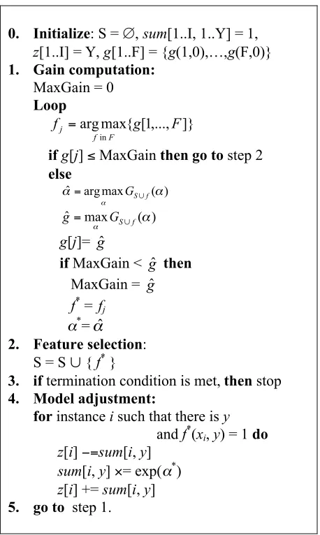
uni-form distribution. The other steps for computing the gains and selecting the features are given in Figure 2 as a pseudo code. Because we only com-pute gains for a small number of top-ranked fea-tures, we call this feature selection algorithm as Selective Gain Computation (SGC) Algorithm.
In the algorithm, we use array g to keep the
sorted gains and their corresponding feature indi-ces. In practice, we use a binary search tree to maintain the order of the array.
The key difference between the IFS algorithm and the SGC algorithm is that we do not evaluate all the features for the active model at every stage (one stage corresponds to the selection of a single feature). Initially, the feature candidates are or-dered based on their gains computed on the uni-form distribution. The feature with the largest gain gets selected, and it forms the model for the next stage. In the next stage, the gain of the top feature in the ordered list is computed based on the model just formed in the previous stage. This gain is compared with the gains of the rest features in the list. If this newly computed gain is still the largest, this feature is added to form the model at stage 3. If the gain is not the largest, it is inserted in the ordered list so that the order is maintained. In this case, the gain of the next top-ranked feature in the ordered list is re-computed using the model at the current stage, i.e., stage 2.
This process continues until the gain of the top-ranked feature computed under the current model is still the largest gain in the ordered list. Then, the model for the next stage is created with the
addi-tion of this newly selected feature. The whole fea-ture selection process stops either when the number of the selected features reaches a pre-defined value in the input, or when the gains be-come too small to be useful to the model.
0. Initialize: S = ∅, sum[1..I, 1..Y] = 1,
z[1..I] = Y, g[1..F] = {g(1,0),…,g(F,0)}
1. Gain computation:
MaxGain = 0
Loop
argmax{ [1,..., ]} in
F g f
F f
j =
if g[j] £ MaxGain then go to step 2
else
) ( max arg
ˆ a
a
a S f G» =
) ( max
ˆ a
a GS f
g= »
g[j]= gˆ
if MaxGain < gˆ then
MaxGain = gˆ
f* = fj
a*=aˆ
2. Feature selection: S = S » { f* }
3. if termination condition is met, then stop
4. Model adjustment:
for instance i such that there is y
and f*(xi, y) = 1 do
z[i] -=sum[i, y]
sum[i, y] ¥= exp(a*)
z[i] += sum[i, y]
5. go to step 1.
Figure 2: Selective Gain Computation Algo-rithm for Feature Selection
In addition to this basic version of the SGC al-gorithm, at each stage, we may also re-compute additional gains based on the current model for a pre-defined number of features listed right after
feature f* (obtained in step 2) in the ordered list.
This is to make sure that the selected feature f* is
[image:4.612.313.542.150.533.2]4
Experiments
A number of experiments have been conducted to verify the rationale behind the algorithm. In par-ticular, we would like to have a good understand-ing of the quality of the selected features usunderstand-ing the SGC algorithm, as well as the amount of speed-ups, in comparison with the IFS algorithm.
The first sets of experiments use a dataset {(x,
y)}, derived from the Penn Treebank, where x is a
10 dimension vector including word, POS tag and grammatical relation tag information from two
ad-jacent regions, and y is the grammatical relation
tag between the two regions. Examples of the grammatical relation tags are subject and object with either the right region or the left region as the head. The total number of different grammatical tags, i.e., the size of the output space, is 86. There are a little more than 600,000 training instances generated from section 02-22 of WSJ in Penn Treebank, and the test corpus is generated from section 23.
In our experiments, the feature space is parti-tioned into sub-spaces, called feature templates, where only certain dimensions are included. Con-sidering all the possible combinations in the
10-dimensional space would lead to 210 feature
tem-plates. To perform a feasible and fair comparison, we use linguistic knowledge to filter out implausi-ble subspaces so that only 24 feature templates are actually used. With this amount of feature tem-plates, we get more than 1,900,000 candidate fea-tures from the training data. To speed up the experiments, which is necessary for the IFS algo-rithm, we use a cutoff of 5 to reduce the feature space down to 191,098 features. On average, each candidate feature covers about 485 instances, which accounts for 0.083% over the whole training instance set and is computed through:
Â
ÂÂ
=
j j xy
j x y
f
ac ( , )/ 1
,
The first experiment is to compare the speed of the IFS algorithm with that of SGC algorithm. Theoretically speaking, the IFS algorithm com-putes the gains for all the features at every stage.
This means that it requires O(NF) time to select a
feature subset of size N from a candidate feature set of size F. On the other hand, the SGC algorithm considers much fewer features, only 24.1 features
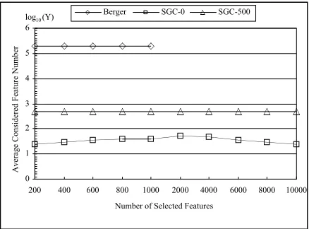
[image:5.612.317.536.339.501.2]on average at each stage, when selecting a feature from the large feature space in this experiment. Figure 3 shows the average number of features computed at the selected points for the SGC algo-rithm, SGC with 500 look-ahead, as well as the IFS algorithm. The averaged number of features is taken over an interval from the initial stage to the current feature selection point, which is to smooth out the fluctuation of the numbers of features each selection stage considers. The second algorithm looks at an additional fixed number of features, 500 in this experiment, beyond the ones considered by the basic SGC algorithm. The last algorithm has a linear decreasing number of features to select, because the selected features will not be consid-ered again. In Figure 3, the IFS algorithm stops after 1000 features are selected. This is because it takes too long for this algorithm to complete the entire selection process. The same thing happens in Figure 4, which is to be explained below.
0 1 2 3 4 5 6
200 400 600 800 1000 2000 4000 6000 8000 10000 Number of Selected Features
Average Considered Feature Number
Berger SGC-0 SGC-500 log10(Y)
Figure 3: The log number of features considered in SGC algorithm, in comparison with the IFS algo-rithm.
-2 -1 0 1 2 3
200 400 600 800 1000 2000 4000 6000 8000 10000
Number of Selected Features
Average Time
for each selection step
(second)
Berger SGC-0
[image:6.612.76.295.74.225.2]log10(Y)
Figure 4: The log time used by SGC algorithm, in comparison with the IFS algorithm.
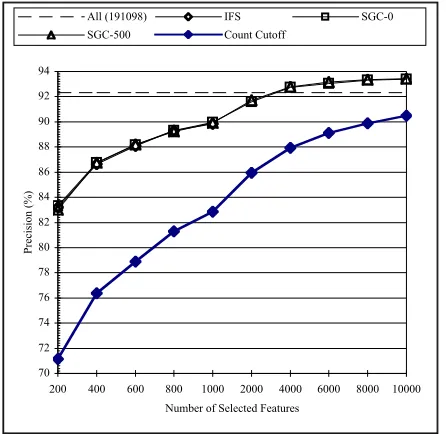
To verify the quality of the selected features using our SGC algorithm, we conduct four experi-ments: one uses all the features to build a condi-tional ME model, the second uses the IFS algorithm to select 1,000 features, the third uses our SGC algorithm, the fourth uses the SGC algo-rithm with 500 look-ahead, and the fifth takes the top n most frequent features in the training data. The precisions are computed on section 23 of the WSJ data set in Penn Treebank. The results are listed in Figure 5. Three factors can be learned from this figure. First, the three IFS and SGC algo-rithms perform similarly. Second, 3000 seems to
be a dividing line: when the models include fewer than 3000 selected features, the IFS and SGC algo-rithms do not perform as well as the model with all the features; when the models include more than 3000 selected features, their performance signifi-cantly surpass the model with all the features. The inferior performance of the model with all the fea-tures at the right side of the chart is likely due to the data over-fitting problem. Third, the simple count cutoff algorithm significantly under-performs the other feature selection algorithms when feature subsets with no more than 10,000 features are considered.
To further confirm the findings regarding preci-sion, we conducted another experiment with Base NP recognition as the task. The experiment uses section 15-18 of WSJ as the training data, and sec-tion 20 as the test data. When we select 1,160 fea-tures from a simple feature space using our SGC algorithm, we obtain a precision/recall of 92.75%/93.25%. The best reported ME work on this task includes Koeling (2000) that has the pre-cision/recall of 92.84%/93.18% with a cutoff of 5, and Zhou et al. (2003) has reached the perform-ance of 93.04%/93.31% with cutoff of 7 and reached a performance of 92.46%/92.74% with 615 features using the IFS algorithm. While the results are not directly comparable due to different feature spaces used in the above experiments, our result is competitive to these best numbers. This shows that our new algorithm is both very effective in selecting high quality features and very efficient in performing the task.
5
Comparison and Conclusion
Feature selection has been an important topic in both ME modeling and linear regression. In the past, most researchers resorted to count cutoff technique in selecting features for ME modeling (Rosenfeld, 1994; Ratnaparkhi, 1998; Reynar and Ratnaparkhi, 1997; Koeling, 2000). A more refined algorithm, the incremental feature selection algo-rithm by Berger et al (1996), allows one feature being added at each selection and at the same time keeps estimated parameter values for the features selected in the previous stages. As discussed in (Ratnaparkhi, 1998), the count cutoff technique works very fast and is easy to implement, but has the drawback of containing a large number of
re-70 72 74 76 78 80 82 84 86 88 90 92 94
200 400 600 800 1000 2000 4000 6000 8000 10000 Number of Selected Features
Precision (%)
All (191098) IFS SGC-0
SGC-500 Count Cutoff
[image:6.612.74.297.444.661.2]dundant features. In contrast, the IFS removes the redundancy in the selected feature set, but the speed of the algorithm has been a big issue for complex tasks. Having realized the drawback of the IFS algorithm, Berger and Printz (1998)
pro-posed an f-orthogonal condition for selecting k
features at the same time without affecting much the quality of the selected features. While this technique is applicable for certain feature sets,
such as link features between words, the f
-orthogonal condition usually does not hold if part-of-speech tags are dominantly present in a feature subset.
Chen and Rosenfeld (1999) experimented on a
feature selection technique that uses a c2 test to see
whether a feature should be included in the ME
model, where the c2 test is computed using the
counts from a prior distribution and the counts from the real training data. It is a simple and probably effective technique for language model-ing tasks. Since ME models are optimized usmodel-ing their likelihood or likelihood gains as the criterion, it is important to establish the relationship between
c2 test score and the likelihood gain, which,
how-ever, is absent.
There is a large amount of literature on feature selection in linear regression, where least mean squared errors measure has been the primary opti-mization criterion. Two issues need to be ad-dressed in order to effectively use these techniques. One is the scalability issue since most statistical literature on feature selection only concerns with dozens or hundreds of features, while our tasks usually deal with feature sets with a million of features. The other is the relationship between mean squared errors and likelihood, similar to the concern expressed in the previous paragraph. These are important issues and require further in-vestigation.
In summary, this paper presents our new im-provement to the incremental feature selection al-gorithm. The new algorithm runs hundreds to thousands times faster than the original incre-mental feature selection algorithm. In addition, the new algorithm selects the features of a similar quality as the original Berger et al algorithm, which has also shown to be better than the simple cutoff method in some cases.
Acknowledgement
This work is done while the first author is visiting the Center for Study of Language and Information (CSLI) at Stanford University and the Research and Technology Center of Robert Bosch Corpora-tion. This project is sponsored by the Research and Technology Center of Robert Bosch Corporation. We are grateful to the kind support from Prof. Stanley Peters of CSLI. We also thank the com-ments from the three anonymous reviewers which improve the quality of the paper.
References
Adam L. Berger, Stephen A. Della Pietra, and Vincent J. Della Pietra. 1996. A Maximum Entropy Approach to Natural Language Processing. Computational Lin-guistic, 22 (1): 39-71.
Adam L. Berger and Harry Printz. 1998. A Comparison of Criteria for Maximum Entropy / Minimum Diver-gence Feature Selection. Proceedings of the 3rd con-ference on Empirical Methods in Natural Language Processing. Granda, Spain.
Stanley Chen and Ronald Rosenfeld. 1999. Efficient Sampling and Feature Selection in Whole Sentence maximum Entropy Language Models. Proceedings of ICASSP-1999, Phoenix, Arizona.
Joshua Goodman. 2002. Sequential Conditional Gener-alized Iterative Scaling. Association for Computa-tional Linguistics, Philadelphia, Pennsylvania. Rob Koeling. 2000. Chunking with Maximum Entropy
Models. In: Proceedings of CoNLL-2000 and LLL-2000, Lisbon, Portugal, 139-141.
Adwait Ratnaparkhi. 1998. Maximum Entropy Models for Natural Language Ambiguity Resolution. Ph.D. thesis, University of Pennsylvania.
Ronald Rosenfeld. 1994. Adaptive Statistical Language Modeling: A Maximum Entropy Approach. Ph.D. thesis, Carnegie Mellon University, April.
J. Reynar and A. Ratnaparkhi. 1997. A Maximum En-tropy Approach to Identifying Sentence Boundaries. In: Proceedings of the Fifth Conference on Applied Natural Language Processing, Washington D.C., 16-19.