Abstract—Principal Component Analysis (PCA) is a
technique to transform the original set of variables into a smaller set of linear combinations that account for most of the original set variance. The data reduction based on the classical PCA is fruitless if outlier is present in the data. The decomposed classical covariance matrix is very sensitive to outlying observations. ROBPCA is an effective PCA method combining two advantages of both projection pursuit and robust covariance estimation. The estimation is computed with the idea of minimum covariance determinant (MCD) of covariance matrix. The limitation of MCD is when covariance determinant almost equal zero. This paper discusses PCA using the minimum vector variance (MVV) to enhance the result. The usefulness of MVV is not limited to small or low dimension data set and to non-singular or singular covariance matrix. The MVV algorithm, compared with FMCD algorithm, has a lower computational complexity; the complexity of VV is of order 0(p2).
Index Term - Determinant, Generalized Variance, Outlier, Principal Component analysis, Robust, Vector Variance.
I. INTRODUCTION
Some practical problems arise in data mining when a large number of variable are measured. This is usually due to the fact that more than one variable may be measuring the same information. The one of variables can be written as a near linear combination of the other variables, and the number of correlated variables will increase when the number of variables increase. To have the good analysis it is necessary to eliminate the redundant information by creating a new set of variables that extract the essential characteristics of the information.
Principal components analysis is a technique to transform the original set of variables into a smaller set of linear combinations that account for most of the original set variance. The basic idea of PCA is to describe the dispersion of an array of n points in p –dimensional space by introducing a new set of orthogonal linear coordinates so that the sample variances of the given points are in decreasing order of dimension, Gnanadesikan (1977).
A principal component analysis focused on reducing the dimensionality of a data set in order to explain as much information as possible. The first principal component is the
First Author is lecturer at Tarumanagara University, Jln Let. Jend. S Parman 1, Jakarta 1140, Indonesia. (e-mail: [email protected]).
Second Author is lecturer at Tarumanagara University, Jln Let. Jend. S Parman 1, Jakarta 1140, Indonesia. (e-mail: [email protected])
combination of variables that explains the greatest amount of variation. The second principal component defines the next largest amount of variation and is independent to the first principal component. This step will be continued for the entire principal components corresponding to the eigenvectors of covariance matrix sample.
The data reduction based on the classical PCA becomes unreliable if outliers are present in the data. The decomposed classical covariance matrix is very sensitive to outlying observations. The first component consisting of the greatest variation is often pushed toward the anomalous observations. Regarding the fact, Huber et al (2003) introduced a new method for robust principal component (ROBPCA).
ROBPCA is PCA method combining two advantages of both projection pursuit and robust covariance estimation. The robust estimator is computed by the MCD ideas of covariance matrix. Based on our experience in computations, ROBPCA is an effective and efficient method. The good properties of ROBPCA tend us to propose the new measure of robust principal component based on minimum vector variance (MVV).
MVV is a measure minimizing vector variance to obtain the robust estimator. The vector variance (VV) is multivariate dispersion that is formulated as Tr
( )
Σ2 , geometrically VV is a square of the length of the diagonal of a parallelotopegenerated by all principal components of XG(Djauhari, 2005). The usefulness of
( )
2Tr Σ is not limited to small or low dimension data set and to non-singular covariance matrix. VV can be used efficiently for very large and high dimension data sets or even for singular covariance matrix. The MVV algorithm, compared with FMCD algorithm, has a lower computational complexity; the complexity of VV is of orderO p( 2). The objective of this paper is to demonstrate the performances of robust principal component using MVV.
II. THE CLASSICAL PRINCIPAL COMPONENT ANALYSIS (PCA)
The principal component analysis is primarily a data analytic technique describing the variance covariance structure through a linear transformation of the original variables. The technique is a useful device for representing a set of variables by a much smaller set of composite variables that account for much of the variance among the set of original variables.
The Robust Principal Component
Using Minimum Vector Variance
Suppose that the random vector XG of p components has the classical covariance matrix S which is a p p×
symmetric and positive semi definite. Covariance matrixScan be reduced to a diagonal matrix Lwhich is a particular orthogonal matrix U such that U SU′ =L
The diagonal elements ofL,λ λ1, 2,",λp, are called the characteristic roots or eigenvalues of S, the columns of U
are called the characteristic vectors or eigenvectors of S. For λ1≥λ2≥ ≥" λp , the principal components are uncorrelated linear combinations YG whose variances are as large as possible. The first principal component is given by
1 1
YG=U XG′ which has the largest proportion of total variance.
The proportion of total variance the k principal component is often explained by the ratio of the eigenvalues
k
λ = k i
i i
λ
=
∑
. The determination of k is an important role to the PCA analysis. A larger k gives a better fit in PCA, but a larger k has the larger redundancy of information. The replacement of original variable p to the k principal component must be considered as a goal in optimizing.The decomposed classical covariance matrix S is very sensitive to outlying observations. The k principal component becomes unreliable if outliers are present in the original variablep. The k principal component consisting of the largest proportion of total variance Sis often pushed toward the outliers.
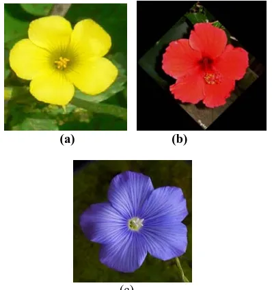
The following application is one of the examples of PCA which is classical to the process of clustering flowers. There are three categories of flowers; red color for Red Hisbiscus, Purple color for Linum Narbonense, and yellow color for Oxalis Pes-Caprae Each pixel of the image can be represented as a point in a 3D RGB color space. The visual contents of the images are extracted and described by color feature vectors.
(a) (b)
(c)
Figure 1. The Images of Flower (a) Oxalis Pes-Caprae, (b) Red Hisbiscus and (c) Linum Narbonense
[image:2.612.335.516.157.284.2]Figure 1 illustrates the flowers. We can easily categorize these three flowers by their colors although they have almost no different shapes. The classical PCA will be used to cluster the flowers. Table 1 contains the ordered λ and cumulative proportion of λ. The result of the clustering involving the three largest or biggest components with cumulative proportion of 91% total of variation turns out to show a’ bad ‘ clustering
Table 1. The Eigen Value of λ
Ordered λ Cumulative Proportion of λ
4.1296 0.459
3.1250 0.806
0.9316 0.910 *
0.5320 0.969
0.1638 0.987
0.0686 0.995
0.0332 0.998
[image:2.612.341.514.377.503.2]0.0157 1.000 0.0005 1.000
[image:2.612.84.283.502.714.2]Figure 2 gives the description of categorized flowers based on their colors. The figure explains that the components having the ‘best’ low rank approximation to original data can not separate the three categorized flower colors. To enhance the clustering, the robust PCA will be discussed in the next section.
Figure 2. The Clustering of Flower Using Classical PCA
III. THE ROBUST PCA USING MINIMUM VECTOR VARIANCE (MVV)
Meanwhile CD involves both of them, the structure of variance and covariance. That is way CD has a wider role on application (Djauhari, 2005), including the role on various robust methods. Even though CD has wider applications than TV, but CD has a limitation too.
Alt and Smith (1988) stated that the main limitation lies on the property that CD = 0 when there is a variable of zero variance or when there is a variable which is a linear combination of other variables. Due to this limitation Djauhari (2005) proposed a different concept of multivariate dispersion measure, called the vector variance (VV). Geometrically VV is the square of the length of the diagonal of a parallelotope generated by all principal components of
XG
Suppose XG is a random vector of covariance matrix Σof dimension
(
p×p)
where λ1≥λ2≥"≥λp ≥0 are eigen values of Σ,11 12 1
21 22 2
1 2
p p
p p pp
σ
σ
σ
σ
σ
σ
σ
σ
σ
⎡ ⎤
⎢ ⎥
⎢ ⎥
Σ =⎢ ⎥
⎢ ⎥ ⎢ ⎥ ⎣ ⎦ " " # # # # "
The structure of TV, GV (CD) and VV can be formulated as,
TV = Tr
( )
Σ = λ1+ λ2 + " + λp (1) CD = Σ = λ λ1 2 " λp (2)VV=
( )
2 2 2 21 2 p
Tr Σ =λ +λ +"+λ (3) Computations of VV are very efficient. The efficiency of VV is of order
( )
2O p compare with CD by using Cholesky decomposition which is of order
( )
3O p .
Regarding the efficient computation of VV, Herwindiati et al (2007) proposed VV in obtaining the robust estimator by minimizing vector variance. The algorithm of MVV has no significant difference to Rousseeuw and van Driessen’s FMCD (1999) except that the criterion used here is not MCD but MVV.
In the outlier labeling process, MVV is an effective and an efficient method, but MVV still takes a few more times in the computation when the dimension p is larger than 100; that is around 110.531. Huber et al (2003) introduced a new method for robust principal component (ROBPCA). ROBPCA is PCA method which combines two advantages of both projection pursuit and robust covariance estimations. The robust estimator is computed by the MCD ideas. Based on our experience of computations, ROBPCA is an effective and an efficient method. The good properties of ROBPCA tend us to propose the new measure of robust principal component based on minimum vector variance (MVV). The algorithm of MVV robust PCA is composed as follows, Stage 1. Start with a singular value decomposition of the mean centered data matrix
, 1 , ,
n p n n r r r r p
X − X =U L V× ′
G G
, with U U′ =Ir =V V′ , X
G
is classical mean vector, L is an r r× diagonal matrix, and Ir is the r r× identity matrix. To optimize the result, we chose k=1 as the principal component consisting of the major part of total variance.
Stage 2. Estimate the location and covariance matrix using MVV robust approach.
1. Let Hold be an arbitrary subset containing 1
2
n k
h= ⎢⎡ + + ⎤⎥
⎣ ⎦data points. Compute the mean vector
old
H
X
G
and covariance matrix
old
H
S of all observations belonging toHold. Then compute,
2old
( )
(
old) (
1old old)
tH i H H i H
d i = X −X S− X −X
G G
G G
for all i = 1, 2, … , n
2. Sort these distances in increasing order,
( )
(
)
(
( )
)
(
( )
)
2 2 2
1 2
old old old
H H H
d π ≤d π ≤"≤d π n
3. Define Hnew =
{
Xπ( )1 ,Xπ( )2 , ,Xπ( )h}
G G G " 4. Calculate new H X G , new H
S and 2
( )
new
H
d i .
5. If Tr S
(
H2new)
= 0, repeat steps 1 to 5. If(
2)
new
H
Tr S =
( )
2old
H
Tr S , the process is stopped.
Otherwise, the process is continued until the k-th iteration if
( )
2( )
2( )
2( )
2( )
21 2 3 k k1
Tr S ≥Tr S ≥Tr S ≥"≥Tr S =Tr S+ Stage 3. Identify the labeled outlier by using robust MVV distance.
Let TMVV
G
and SMVV be the location and covariance matrix given by that process. Robust squared Mahalanobis distance is defined as,
2
(
) (
)
1(
)
, t
MVV i MVV i MVV MVV i MVV
d XG TG = XG −TG S− XG −TG for all i = 1, 2, … , n.
Observations which have a large distance
(
)
2 ,
MVV i MVV
d XG TG will be labeled as outliers or suspects. Compared to FMCD algorithm, the MVV algorithm has a lower computational complexity. As VV is the sum of square of all elements of the covariance matrix, the computational complexity of VV is of order 2
( )
O p . On the other hand, based on Cholesky decomposition for large value of p, the number of operations in the computation of CD is equal to
1
1
( 1) ( 1) ( 1)( )
p
i
p p p p p i p i
−
=
+ − + −
∑
− − −which is of the order ofO p( 3).
subset h=max
{
[ ]
αn ,⎣⎡(
n+kmax+1 / 2)
⎤⎦}
, where α is chosen as any real value between 0.5 and 1, kmax as a maximal number of components that will be computed. In this paper we chose 12
n k
h= ⎢⎡ + + ⎤⎥
⎣ ⎦.
The choice of this subset is due to the ‘reality’ of breakdown points that are found in our computation experience. Compared to the other subset h, the breakdown
point of 1
2
n k
h= ⎢⎡ + + ⎤⎥
⎣ ⎦ is more stable. The following figure
[image:4.612.79.294.28.552.2]reveals the fact.
Figure 3. MVV Breakdown point using 1
2 n k h= ⎢⎡ + + ⎤⎥
[image:4.612.311.540.45.129.2]⎣ ⎦
Figure 4. MVV Breakdown point using h=0.75n
IV. THE PERFORMANCEOFMVVROBUSTPCA
A. The Clustering Flower Images
[image:4.612.331.522.243.383.2]This section discusses the work of MVV through the example of flowers clustering in Section 2. We will categorize the flowers according to their colors; 40 images of Red Hisbiscus, 15 images of Linum Narbonense, and 19 images of Oxalis Pes-Caprae. The color moment is used in order to get the color feature of those flowers,. The extraction of each pixel in the color feature is represented as a point in a 3D RGB color space .
Figure 5. The Images of Flower (a) Oxalis Pes-Caprae, (b) Red Hisbiscus and (c) Linum Narbonense
[image:4.612.86.283.267.534.2]MVV robust PCA is used to cluster the flowers based on their color. The excellent result of clustering can be seen in Figure 6. Every flower is perfectly categorized into its group, as can be seen below,
Figure 6. Scatter Plot of Clustering Flower Images
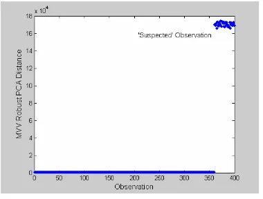
B. The Identification of Anomalous Data in High and Large Dimension.
MVV Robust PCA also works well in the process of identification of anomalous data in high and large dimension, assuming that anomalous data is suspected as outlier. For this purpose, we generate n=400 random data from a mixture of p-variate normal distribution
(
1−ε)
Np(
µ1,Ip)
+ε Np(
µ2,Ip)
G G
with p=300; ε =0.1 where µ =1 0
G G
, µ =2 10e
G G
and eG = eG=
(
1 1" 1)
t is of pdimension
[image:4.612.90.281.407.543.2] [image:4.612.339.529.550.694.2]The identification process is done quite well by MVV robust PCA. The suspected outliers can be clearly separated and is located far away from the group of clean data. The separating process needs only less than 4 seconds
C. The Computation time of MVV Robust PCA
Hubert et al (2003) described that the computation of ROBPCA on Pentium IV with 2.40 GHz is 3.06 seconds for
39, 226
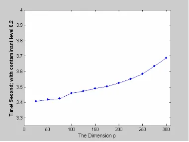
n= p= and 3.19 seconds for n=111,p=11 . Compared to ROBPCA, the computation time of MVV robust PCA is not slower. To see the time effectiveness of MVV robust PCA can be seen in the following figures which show that the computation process between the dimensional data of p=25 to p=300 with n= 100, 0.1ε = ,
and ε =0.2 from a mixture model
(
1−ε)
Np(
µ1,Ip)
+ε Np(
µ2,Ip)
[image:5.612.336.518.46.183.2]G G
[image:5.612.79.291.140.392.2]Figure 8. The Computation Time of MVV with Contaminant Level ε =0.1
Figure 9. The Computation Time of MVV with Contaminant Level ε =0.2
[image:5.612.90.280.441.584.2]The figures show that the additional contaminant ε and also the change of p dimension does not produce a significant difference in time. Even if we compare the amount of contaminant ε =0.1and ε =0.4for the same dimension, we find no significant difference, see Figure 8 and Figure 10.
Figure 10. The Computation Time of MVV with Contaminant Level ε =0.4
V CONCLUSION
MVV robust PCA is an effective and an efficient method to identify outlier in a high and large dimension. MVV robust PCA is also an impressive method for interpreting the application of PCA, such as the clustering process. From the aspects of computation of several p- dimensions, MVV robust PCA gives the promising results.
REFERENCES
[1] Alt, F.B. and Smith, N.D.: Multivariate Process Control, Handbook of Statistics, 7, 333-351 (1988)
[2] Anderson, T.W.: An Introduction to Multivariate Statistical
Analysis, Second Edition, John Wiley, New York (1984)
[3] Djauhari, M.A.: Improved Monitoring of Multivariate Process
Variability, Journal of Quality Technology, Vol. 37, No 1, 32-39
(2005)
[4] Gnanadesikan, R.: Method for Statistical Data Analysis of
Multivariate Observations, John Wiley, New York (1977)
[5] Hawkins, D.M.: The Feasible Solution Algorithm for the Minimum Covariance Determinant Estimator in Multivariate Data, J.Computational Statistics and Data Analysis, 17, 197-210 (1994) [6] Herwindiati, D.E., Djauhari, M.A. and Mashuri, M.:Robust
Multivariate Outlier Labeling, J. Communication in Statistics –
Simulation And Computation, Vol. 36, No 6 (2007)
[7] Hubert, M., Rousseeuw, P.J. and vanden Branden, K.: ROBPCA: a
New Approach to Robust Principal Component Analysis, J.
Technometrics, 47, 64-79, (2005)
[8] Johnson, R.A. and Wichern, D.W.: Applied Multivariate Statistical
Analysis, Second Edition, John Wiley, New York (1988)
[9] Long, F., Zhang, H. and Feng, D.D.: Multimedia Information
Retrieval and Management, Spinger, Berlin (2003)
[10] Rousseeuw, P.J. and van Driessen, K.: A Fast Algorithm for The
Minimum Covariance Determinant Estimator, J. Technometrics,