H}istogram Partitioning for Feature Vector Dimension Reduction in Bins Approach for {CBIR

(1)

Histogram Partitioning for Feature Vector Dimension

Reduction in Bins Approach for CBIR

Dr. H. B. Kekre

Sr. Professor

Kavita Sonawane

Ph.D. Research Scholar

Abstract—Feature vector dimensionality is an important issue in any CBIR system. It has great impact on the execution time required by the system to process the given query and generate the retrieval results. We have introduced a novel idea in this paper to extract the feature vectors of the image along with dimensionality reduction. It gives the improved performance as compared to already existing methods. The approach used is called bins approach; designed and implemented using image histogram partitioning. Three image histograms are obtained for each image plane R, G and B separately. Each of them is partitioned using two different techniques namely LP-Linear partitioning and CG –Centre of Gravity partitioning. Performance of these two partitioning techniques is compared by taking 4 different cases into consideration. Four different cases implemented in this paper are based on the variations used in the techniques to extract the image features. Multiple feature vector databases are prepared as pre-processing part of this work. Feature extraction techniques used are based on the original-ORG as well as equalized histogram-EQH and their partitioning based on LP and CG. This partitioning generates 8 bins holding the count of the pixels based on the color contents of the image. Further these 8 bins data is processed by computing the first four statistical moments (Mean, Standard deviation-STD, Skewness-SKEW, and Kurtosis- KURTO) representing the feature vectors of dimension 8. Retrieval results obtained by comparing the query image with database feature vectors by means of three similarity measures Euclidean distance (ED), Absolute distance (AD) and Cosine correlation distance (CD).

Keywords — CBIR, Bins, Linear Partitioning, CG Partitioning, Mean, Standard Deviation, Skewness, Kurtosis.

I. I

NTRODUCTION

This Paper explores the new idea for extracting the feature vectors giving improved performance along with the dimensionality reduction. Development of efficient feature extraction methods and selection of proper similarity metric are important aspects for the successful CBIR system [1][2][3]. Various images feature are classified into local and global image features. It includes low level image features like color, shape, texture and also the various image content descriptors color histograms, fuzzy histograms can be computed using basic image contents. Several methods for retrieving images on the basis of colour have been described in the literature, but most are variations on the same basic idea [4][5][6]. Color features are widely used in CBIR systems. Color features can be defined in various color spaces as per the use for different application [7]. Developing the efficient feature

given query [8][9]. There are various techniques implemented by CBIR researchers in frequency and spatial domain of image processing field to extract the image features. Spatial domain techniques includes the use of histograms [10][11]. We are focusing on the use of image histograms to extract the image features and also trying to reduce the size of the feature vector. Image histogram shows the total tonal distribution in the image. It is a bar chart of the count of pixels of every tone of gray that occurs in the image. The histogram is used and altered by many image enhancement operators. Histogram equalization is one of them; based on the assumption that image has to use full intensity range to display maximum contrast [12][13]. We have used histogram equalization in our work before partitioning the histogram to generate the bins and check its effect; which is reflected in the results and discussion. In this work we are mainly focusing on dimensionality reduction of the feature vector using bins approach. As we are using histogram, by default it gives 256 bins for intensity range 0-255. Use of 256 bins as a feature vector increases the time and space complexity [14][15]. To overcome this drawback we are working on reducing the feature vector size along with the improvement in the similarity retrieval [16][17][18].

Feature extraction explained in this paper includes bins formation by partitioning of original and equalized histogram of R, G and B image planes into two parts using two techniques; linear and CG partitioning. Two partitions for three planes leads to generation of 8 bins. Once the bins are ready, data contained in the bins is processed by computing the statistical first four moments for them. The first four moments; Mean, standard Deviation (STD), Skewness (SKEW) and Kurtosis (KURTO) extracted from 8 bins pixel data forms the 4 types of feature vector of dimension 8. These features are extracted separately for R, G and B color contents of the image. Based on the types of feature vectors we have prepared total 12 feature vector databases for 2000 database images. This process is followed with both partitioning techniques for both type of histograms i.e for original and equalized histogram. This leads to the generation of multiple feature vector databases i.e. 192 feature databases with all possibilities tried.

(2)

out using database of 2000 BMP images includes 20 classes, in which few of them are taken from Wang database[21].

Work done for the proposed system presented in this paper is organized as follows. Section I gives the introduction of the system, Section II Histogram with Equalization. Partitioning techniques are discussed in section III. Preprocessing work for feature databases is elaborated in Section IV. Section V defines the similarity measures and evaluation parameters used in the system. Experimental Results are discussed in section VI which is flowed by conclusion in section VII.

II. H

ISTOGRAM AND

H

ISTOGRAM EQUALIZATION

Histogram gives summary of count of pixels in the number of bins. Histogram bins are representing the no of grey levels in the image. By default Matlab generates 256 bins for the image histogram. It represents 0 to 255 intensity levels of the image. Bin pixel count means count of pixels having same grey level or intensity will appear in the same bin. For bins having count zero can be interpreted that image does not contain the pixels of that particular intensity (bin). Normal or say original image histogram shows the distribution of pixels in 256 bins according to the intensity they carry without manipulating the original intensity values.

We have thought of modifying the image histog ram so that we can have uniform distribution of the pixels across 256 intensities (bins). To promote this modification we have used histogram equalization and we have checked its performance for the CBIR.

These two histograms are partitioned using linear and CG partitioning techniques. Partitioning has variable impact on the feature vectors and in turn on the retrieval results. We have compared the results with respect to partitioning techniques used for the original (ORG) as well as equalized (EQH) histogram.

Fig.1. Shows the image with RGB planes and Fig.2. Shows the original and equalized histograms of R, G and B planes.

Fig.1. Pyramid Image with R, G and B Planes

Fig.2. Pyramid Image with R, G and B Original and Equalized Histograms

III. P

ARTITIONING

T

ECHNIQUES

As discussed in the introduction, we are concentrating on the feature vector dimensionality reduction; we have used two partitioning techniques to divide the histograms into two parts.

We are avoiding the use of 256 bins of histogram to be selected as feature vector because of time and space complexity. Division of histogram in two partitions for the R, G and B planes leads towards generation of just 8 bins. These 8 bins are used as feature vector rather than using the 256 bins of histogram.

A. Linear Partitioning

:

LP

Linear Partitioning is simple partitioning technique which divides the total number of pixels of image into two equal parts. The grey level at which this partitioning occurs, acts as threshold for the pixels to be counted in two parts identified as part 0 and part1. Fig. 3 a and b. Shows linear partitioning in black color for original and equalized histogram respectively.

B. Centre of Gravity Partitioning: CG

After applying linear partitioning we found that it is actually giving unbalanced partitioning because it takes only the count of pixels into consideration, ignoring the intensity values. But in CG we are giving equal importance to the pixels and their intensities. These intensities are considered as weight of the pixels so that according to their weights we are dividing the pixels into two parts by computing the CG. By computing CG we can obtain two partitions identified as part0 and part1 such that the both partitions will have same weight (intensities). This partitioning gives improvement in the retrieval performance of the system as compared to LP. Fig 3a and b. Shows the CG partitioning of original and equalized histogram respectively in blue color. We use following equation 1 to compute CG.





    

 

    

 

 

  



n

i i

W

n W n L W

L W L CG

1 ... 2 2 1

(3)

Fig.3.a. Original with CG (in Blue) and LP (in Black) Partitioning

Fig.3.b. Equalized Histogram with CG (in Blue) and LP(in Black) Partitioning

IV. F

EATURE

V

ECTOR

D

ATABASES

: P

RE

-PROCESSING

W

ORK

As discussed earlier feature extraction and selection of similarity metric are important stages of any CBIR system. We have achieved reduction in the feature dimension by two partitioning techniques applied on histograms and dividing them into two parts and forming bins out of them. The process of bins formation and preparing the multiple feature vector databases is explained in following parts A and B.

A. Bins Formation: 8 Bins

This process starts with separation of an image into R, G and B planes. For each plane two histograms are obtained original and equalized histogram. These histograms are then partitioned into two parts namely part0 and part1 by LP and CG techniques.

Now, three histograms R, G and B each with two partitions 0 and 1 leads to generation of 8 bins as follows:

First, Pick up the pixel from an image under feature extraction process, check its R, G and B intensities so that which of the two (Part 0 or 1) partitions of respective R, G and B histogram it falls will be assigned to that pixel as flag.

Let, the pixel under process has R, G and B intensities falling in range of parts 0, 1and 1 of the respective histograms; then that pixel will be counted in bin number

the feature vector of just 8 components from the three histograms of sized 256 bins. Example 8 bins for same pyramid image are shown in Fig.4.

Fig.4. Sample 8 Bins Containing Count of Pixels for Pyramid Image

Each bin in above image is labelled with the count of pixels it has. Bin 3 is showing ‘0’, it means no of pixels with flag ‘011’ falling in partition 0,1 and 1 for R, G and B values respectively are not present in the image. We can interpret that count of pixels in bins3 is zero.

B. Multiple Feature Vector Databases

Once we obtain the count of pixels into 8 bins, this information is used to compute the feature vectors. We have considered RGB intensities of the pixels counted into 8 bins and computed first 4 moments for them. Moments computed and stored separately as feature vector in separate database namely MEAN, STD, SKEW and KURTO for R, G and B separately. This way we get 12 feature databases for 1 partitioning technique with one histogram.

While partitioning the histograms we thought of taking 4 different cases into consideration so that the system proposed in this paper can be evaluated through all the possible cases to recommend precise partitioning leads to reduce the size of the feature vector. Based on the LP and CG partitioning of the ORG and EQH histograms we have worked out the following 4 cases for each partitioning technique as given below

Note: (FV-feature Vector, LP Linear partitioning, CG-Centre of Gravity, ORG–Original, EQH- Equalized)

LP Partitioning

Case1 : LP on ORG and FV Extracted from ORG Case2 : LP on EQH and FV Extracted from EQH Case3 : LP on ORG and FV Extracted from EQH Case4 : LP on EQH and FV Extracted from ORG

CG Partitioning

Case1 : CG on ORG and FV Extracted from ORG Case2 : CG on EQH and FV Extracted from EQH Case3 : CG on ORG and FV Extracted from EQH Case4 : CG on EQH and FV Extracted from ORG

(4)

V. S

IMILARITY

M

EASURE AND PERFORMANCE EVALUATION

As discussed earlier after feature extraction, the second important aspect to be considered for CBIR is selection of similarity measure. It compares the query image feature vector with the database feature vectors and calculates the distance between them. Calculating distance is nothing but finding similarity between the query and database images. Images closer to query will be selected for the final retrieval. Retrieval set may contain images relevant to query and irrelevant to query as well. It becomes an important issue to be handled in CBIR to analyse the results so that performance of the CBIR system can be evaluated and strength of the system in retrieving the similar images will be delineated.

A. Similarity Measure

To facilitate the comparison process we have used three similarity measures namely Euclidean distance (ED), Absolute distance and Cosine Correlation distance (CD) shown in equations 2, 3 and 4 respectively. Each of them has their own features and they are performing better in different factors.

Euclidean Distance





(2)

2

1





  n

i

i i

QI FQ FI

D

Absolute Distance:

) 3 ( )

( 1

i n

i i

QI FQ FI

D 







Cosine Correlation Distance





(4)

) ( ) ( ) ( ) (

) ( ) (

n Q n Q n D n D

n Q n D

‘Where D(n) and Q(n) are Database and Query feature Vectors resp.

When query image is fired to the system; feature extraction is carried out for it and the comparison process starts and distance between query and database feature vectors is calculated using the equations 2, 3 and 4. These distances are then sorted in ascending order from (min. distance to max.).

Usually retrieval set is prepared by selecting the images closer to query from the sorted distances. To decide this, a threshold is selected on trial and error basis [22][23]. But this is time consuming method of selecting the threshold on trial and error basis which may not give uniform performance for all types of queries. In our case instead of selecting threshold on trial and error basis we are taking first 100 images from the sorted distances (2000 in our database) to be selected as set similar images to be retrieved. This is because we have total 100 images of each in the database.

Performance evaluation parameters used for the proposed system are illustrated in next section.

B. Performance Evaluation Parameters

We have used three parameters to evaluate the system performance that are PRCP, LS and LSRR and are defined as follows.

1. PRCP: Precision Recall Cross over Point.

Many researchers have used two conventional parameters precision and recall for the CBIR evaluation [23][24].

Precision is fraction of relevant images retrieved to all images retrieved for the given query.

Recall is fraction of relevant images retrieved to all relevant images in the database.

In both cases, we can see that, user is always interested in images to be retrieved which are relevant query either from the database or from all retrieved. Precision and recall both should be as high as possible as per user’s expectations. Taking this into consideration, we are using parameter PRCP which is actually a cross over point of precision and recall, where both have same value. In our case we are selecting initial string of length equal to the no of relevant images in the database to get the PRCP value. PRCP = 1; indicates the ideal performance of the system; which means all the relevant images in the database are retrieved as initial string.

PRCP = 0; indicates the worst case system performance ; which means that no relevant image is retrieved and PRCP between 0 to 1 tells us that how far we are from the ideal system.

2.LS : Longest String

Longest string is the parameter which retrieves the continuous string of relevant images from the sorted set of distances (2000 in this experiment). This value is expected to be as high as possible.

3.LSRR : Length of String to Retrieve all Relevant

This parameter measures the length of string traversed by the system to collect all images from database relevant to query from the set of sorted distances. Minimum length indicates that system is performing better, takes less time and traversal to collect all query relevant images from database. Maximum LSRR shows worst case performance of the system.

VI. E

XPERIMENTAL RESULTS AND

D

ISCUSSION

The work presented in this paper is experimented with database of 2000 BMP images from 20 different classes. As part of pre-processing work we have prepared total 192 feature vector databases for 2000 database images. It covers all the 8 cases discussed in section IV B used in the feature extraction method based on the histograms and two partitioning techniques for bins formation.

A. Database and query Images

(5)

Fig.5. Sample Images from 20 classes in Database Next phase after feature extraction, the system enters in is, comparing the query and database image features. We have used set of 200 query images to check the system performance and response with proposed methods illustrated through 8 different cases. It includes 10 images selected randomly from 100 images of each of the 20 classes.

B. Results and Discussion

We have executed same set of 200 queries for 192 feature vector databases and compared the performance using all the performance evaluation parameters PRCP, LS and LSRR as discussed in section V–B.

Results presented in this section elaborating the system performance for all factors based on the type of the feature vector i.e. MEAN STD, SKEW and KURTO for R, G and B colors separately. It also presents and compares the results on the basis of histogram partitioning techniques used for bins formation. From total 8 cases, cases from both partitioning techniques are compared simultaneously as follows in following tables from I to XXII.

C. PRCP:

Case1 : LP on ORG and FV Extracted from ORG Case 1 : CG on ORG and FV Extracted from ORG

Table I. Case1: MEAN

ED AD CD

CG LP CG LP CG LP

R 5567 5607 5848 5644 5651 5728

G 5384 5472 5485 5450 5751 5853

B 5264 5342 5387 5379 5210 5245

Table II. Case 1: STD

ED AD CD

CG LP CG LP CG LP

R 6046 6234 6292 6526 5604 5736

G 6277 5799 6422 5933 6147 5767

B 5700 5570 5848 5858 5485 5445

Table III Case 1: SKEW

ED AD CD

CG LP CG LP CG LP

R 4576 5011 4907 5491 4330 5224

G 4984 4711 5264 5190 4806 5111

B 4799 4737 5107 5100 4658 4998

R 6096 6297 6311 6560 5813 5920

G 6704 6081 6868 6300 6344 5846

B 6045 5681 6191 5885 5733 5607

Case2: LP on EQH and FV Extracted from EQH Case2: CG on EQH and FV Extracted from EQH

Table V. Case2 : MEAN

ED AD CD

CG LP CG LP CG LP

R 4656 4737 4595 4690 4387 4504

G 5024 5232 5136 5264 4700 5005

B 4619 4641 4596 4548 4298 4283

Table VI.Case 2: STD

ED AD CD

CG LP CG LP CG LP

R 4794 4586 4877 4594 4785 4708

G 5361 5116 5403 5128 5411 5232

B 5006 4634 5056 4663 5181 4799

Table VII. Case 2: SKEW

ED AD CD

CG LP CG LP CG LP

R 3863 3702 3965 3755 3441 3460

G 4372 4151 4583 4254 3950 3912

B 4403 4044 4566 4115 3906 3660

Table VIII. Case 2: KURTO

ED AD CD

CG LP CG LP CG LP

R 4882 4738 4987 4768 4836 4751

G 5625 5305 5682 5366 5536 5359

B 5292 4885 5281 4891 5364 4953

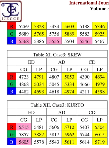
Case3 : LP on ORG and FV Extracted from EQH Case3 : CG on ORG and FV Extracted from EQH

Table IX Case3: MEAN

ED AD CD

CG LP CG LP CG LP

R 5064 4777 5230 5142 4789 4786

G 5494 5329 5543 5357 5528 5395

B 5175 4916 5259 5168 5041 4939

(6)

R 5269 5328 5434 5603 5138 5346

G 5689 5765 5756 5889 5583 5925

B 5568 5386 5555 5504 5546 5467

Table XI. Case3: SKEW

ED AD CD

CG LP CG LP CG LP

R 4723 4791 4807 5053 4390 4694

G 4868 5034 5045 5334 4666 4979

B 4482 4693 4618 4974 4211 4598

Table XII. Case3: KURTO

ED AD CD

CG LP CG LP CG LP

R 5515 5481 5606 5712 5407 5504

G 5857 5882 5817 5962 5744 6015

B 5605 5578 5543 5611 5614 5719

Case4 LP on EQH and FV Extracted from ORG Case4 CG on EQH and FV Extracted from ORG

Table XIII. Case 4 : MEAN

ED AD CD

CG LP CG LP CG LP

R 4820 5607 5578 5644 4448 5728

G 4922 5472 5455 5450 4786 5853

B 4535 5342 5037 5379 4308 5245

Table XIV. Case4 : STD

ED AD CD

CG LP CG LP CG LP

R 7161 6234 7241 6526 6734 5736

G 6651 5799 6856 5933 5965 5767

B 5841 5570 6118 5858 5604 5445

Table XV. Case4: SKEW

ED AD CD

CG LP CG LP CG LP

R 5167 5011 5426 5491 4885 5224

G 5121 4711 5444 5190 4818 5111

B 5008 4737 5278 5100 4833 4998

Table XVI. Case4: KURTO

ED AD CD

CG LP CG LP CG LP

R 7215 6297 7336 6560 6625 5920

G 7038 6081 7253 6300 6306 5846

B 6245 5681 6460 5885 6019 5607

PRCP results are obtained by executing all 200 query images with 192 feature vector databases. We are specifying only total PRCP obtained for 200 query images for each factor considered to identify the feature vector separately. Each value shown in the table is out of 20,000. Here we are mainly concern with the importance of the histogram partitioning technique to reduce the feature vector size and improve the retrieval performance.

In above tables we can observe that results are highlighted with pink and yellow color. Yellow color is specifically used for LP when it is better than CG and Pink color is used for CG to show when CG is better than LP.

When we see these highlighted results, we can say that, CG is the best partitioning for histogram to reduce the no of bins and improve the retrieval of similar images. If we analyse these results case wise for 4 cases with two partitioning, we have obtained the following analysis details in brief.

Table XVII.

Analysis CG LP

Case 1 18 18

Case 2 28 8

Case 3 25 11

Case 4 14 22

Overall Score:

144 85 59

Above details are indicating that total 144 PRCP results compared for the performances against each other; amongst them CG is better than LP for 85 places. Means CG is performing far better than LP and giving very good retrieval results. The best results obtained among these results for each moment with respect to each factor are shown in table XVIII.

Table XVIII: BEST RESULTS

Moment CASE 1 CASE 2 CASE 3 CASE 4

MEAN 5848 AD

CG

5264 AD LP

5543 AD CG

5853 CD LP

STD 6526 AD

LP

5411 CD CG

5889 AD LP

7241 AD CG

SKEW 5491 AD

LP

4583 AD CG

5334 AD LP

5491 AD LP

KURTO 6868 AD

CG

5682 AD CG

6015 CD LP

(7)

we have combined these results using OR operation applied over R, G and B results obtained separately.

Table XIX. CASE 1 : 'R' OR 'G' OR 'B'

CASE 1

ED AD CD

CG LP CG LP CG LP Mean 8859 8622 9192 8669 8914 8564

STD 10256 9950 10404 9943 9989 9181

SKEW 9248 8868 9522 9170 8844 8803

KURTO 10678 10076 10826 10084 10218 9320

Table XX. CASE 2 : 'R' OR 'G' OR 'B'

CASE2

ED AD CD

CG LP CG LP CG LP

Mean 7800 7960 7791 7902 7440 7691

STD 8862 8623 8892 8537 8958 8735

SKEW 8153 7688 8210 7676 7726 7333

KURTO 9193 8907 9222 8851 9178 8960

Table XXI. CASE 3 : 'R' OR 'G' OR 'B'

CASE 3

ED AD CD

STD 10592 10422 10635 10325 9950 9748

SKEW 9640 9474 9715 9407 9175 8934

KURTO 10774 10576 10803 10477 10064 9981

Table XXII. CASE 4 : 'R' OR 'G' OR 'B'

CASE 4

ED AD CD

CG LP CG LP CG LP

Mean 8125 7693 8039 7583 8182 7953

STD 9307 9008 9177 8942 9367 9074

SKEW 8819 8825 8718 8847 8664 8638

KURTO 9577 9291 9325 9112 9608 9359

Observing above tables we can notice that we could really improve the retrieval by very good amount in all the results. In all four cases. Here also when we are comparing the two partitioning techniques we found that, CG is (marked with pink color) far better than LP in maximum results (43 out of 48 cases) with respect to all other parameters like distance measure and type of moment. All PRCP values have crossed 8000 except few results of Case 3. Among these results, the best results obtained for PRCP are highlighted with green color. The highest value we

PRCP for 200 query images. This is very good achievement for us in the CBIR field.

The next two parameter we have used to evaluate the performance of our system is LS and LSRR. As discussed earlier LS is the continuous longest string of relevant images and should be as high as possible. Whereas LSRR is the length to be travelled to collect all query relevant images from database and should be as low as possible. Taking these factors into consideration as user’s point of view; we have executed all 200 queries over 192 feature vector databases but taken only maximum and minimum among those results for LS and LSRR respectively. Parameters, LS and LSRR are also compared with respect to the two partitioning techniques using 4 cases considered so far. Results obtained for LS and LSRR are shown as follows. Chart 1 to 8 is showing LSRR and LS for Case 1 to case 4 respectively.

CASE 1

ED AD CD

STD 10256 9950 10404 9943 9989 9181

SKEW 9248 8868 9522 9170 8844 8803

KURTO 10678 10076 10826 10084 10218 9320

CASE2

ED AD CD

CG LP CG LP CG LP

Mean 7800 7960 7791 7902 7440 7691

STD 8862 8623 8892 8537 8958 8735

SKEW 8153 7688 8210 7676 7726 7333

KURTO 9193 8907 9222 8851 9178 8960

CASE 3

ED AD CD

STD 10592 10422 10635 10325 9950 9748

SKEW 9640 9474 9715 9407 9175 8934

KURTO 10774 10576 10803 10477 10064 9981

CASE 4

ED AD CD

CG LP CG LP CG LP

Mean 8125 7693 8039 7583 8182 7953

STD 9307 9008 9177 8942 9367 9074

SKEW 8819 8825 8718 8847 8664 8638

KURTO 9577 9291 9325 9112 9608 9359

0 5 10 15 20 25 30 35 40 45

CG LP CG

ED AD

Chart 1: LSRR for Case 1: Partitioning of ORG FV from ORG

MEAN STD

CG LP CG

ED

MEAN 92 81 88

STD 47 61 48

SKEW 29 36 27

KURTO 30 58 40 0 10 20 30 40 50 60 70 80 90 100

Chart 2: LS for Case 1: Partitioning of ORG FV from ORG

CASE 1

ED AD CD

STD 10256 9950 10404 9943 9989 9181

SKEW 9248 8868 9522 9170 8844 8803

KURTO 10678 10076 10826 10084 10218 9320

CASE2

ED AD CD

CG LP CG LP CG LP

Mean 7800 7960 7791 7902 7440 7691

STD 8862 8623 8892 8537 8958 8735

SKEW 8153 7688 8210 7676 7726 7333

KURTO 9193 8907 9222 8851 9178 8960

CASE 3

ED AD CD

STD 10592 10422 10635 10325 9950 9748

SKEW 9640 9474 9715 9407 9175 8934

KURTO 10774 10576 10803 10477 10064 9981

CASE 4

ED AD CD

CG LP CG LP CG LP

Mean 8125 7693 8039 7583 8182 7953

STD 9307 9008 9177 8942 9367 9074

SKEW 8819 8825 8718 8847 8664 8638

KURTO 9577 9291 9325 9112 9608 9359

LP CG LP

AD CD

SKEW KURTO

CG LP CG LP

AD CD

88 88 75 58

48 83 41 55

27 62 32 53

40 69 34 54

(8)

In above charts we can observe that, here also CG is performing better as compared to LP in most of the cases. The best LSRR value obtained is 8% i.e only 8% traversal of 2000 images sorted according the distances in 0

10 20 30 40 50 60

CG LP CG LP CG

ED AD

MEAN STD SKEW

CG LP CG LP

ED AD

MEAN 66 34 70 29

STD 61 46 54 47

SKEW 41 36 34 39

KURTO 50 46 62 47 0

10 20 30 40 50 60 70 80

Chart 4: LS for Case 2: Partitioning of EQH FV from EQH

0 10 20 30 40 50 60

CG LP CG LP

Chart 5: LSRR for Case 3: Partitioning of EQH FV from ORG

MEAN STD SKEW

In above charts we can observe that, here also CG is performing better as compared to LP in most of the cases. The best LSRR value obtained is 8% i.e only 8% traversal of 2000 images sorted according the distances in CG LP

CD

SKEW KURTO

LP CG LP

CD

29 61 58

47 56 47

39 34 55

47 54 56

Chart 4: LS for Case 2: Partitioning of EQH FV from EQH

CG LP

Chart 5: LSRR for Case 3: Partitioning of EQH FV from ORG

SKEW KURTO

CG LP CG

ED

MEAN 66 67 70

STD 61 60 54

SKEW 41 33 34

KURTO 50 41 62 0

10 20 30 40 50 60 70 80

Chart 6: LS for Case 3: Partitioning of EQH FV from ORG

0 5 10 15 20 25 30 35 40 45

CG LP CG

ED AD

Chart 7: LSRR for Case 4: Partitioning of ORG FV from EQH

MEAN STD

CG LP CG

ED

MEAN 41 49 45

STD 38 43 38

SKEW 28 27 29

KURTO 38 39 38 0

10 20 30 40 50 60 70

Chart 8: LS for Case 2: Partitioning of ORG FV from EQH

In above charts we can observe that, here also CG is performing better as compared to LP in most of the cases. The best LSRR value obtained is 8% i.e only 8% traversal of 2000 images sorted according the distances in

CG LP CG LP

AD CD

70 70 61 58

54 52 56 54

34 36 34 53

62 45 54 53

Chart 6: LS for Case 3: Partitioning of EQH FV from ORG

LP CG LP

AD CD

Chart 7: LSRR for Case 4: Partitioning of ORG FV from EQH

SKEW KURTO

CG LP CG LP

AD CD

45 49 48 58

38 43 47 57

29 27 48 55

38 39 48 56

(9)

ascending order gives 100% recall. Which means getting all 100 relevant images in first 160 images. Similarly the best value obtain for LS is 92, means we could retrieve 92 images from 100 images of the query class in the database. Observation based on the results obtained by four moments suggests that even moments (STD and KURTO) are performing far better than odd moments (MEAN and SKEW) in terms of retrieval of similar images.

When we observed the performance given by different similarity measures ED, AD and CD, we found that AD and CD are performing far better than that of ED which used by most of the CBIR researchers as per literature survey [25][26].

We have presented the performances by four different cases with respect to the partitioning applied over and pixels picked up from either ORG or EQH for Feature vector formation histogram. Observing the responses given by these four cases for all other parameters, we found that CG is performing better for the cases where CG partitioning is applied over EQH and feature vectors are also formed using the modified equalized image planes. Means when intensities are distributed uniformly and then we are applying the CG partitioning which

gives the two uniformed (having same

moments/weights) partitions have positive impact on the retrieval process.

Observing the results obtained for queries from 20 different classes of database we found that few classes are performing very well. Classes Flower, Sunset, Dinosaur, Barbie, Car, Dove, Kingfisher, Rainbow Rose, Ship, Horses, Waterfall are giving better results for the given queries. A close observation of these classes shows that the color intensities are uniformly distributed leading to better performance as we have focused on the color contents of images.

VII. C

ONCLUSION

CBIR system presented in this paper is based on the bins approach. The 8 bins are formed by partitioning of histogram and used as feature vector of dimension 8.

Idea behind the design of bins approach is to reduce the feature vector dimension so that space and computational complexity can be reduced. We could greatly reduce the size of the feature vector in this work by avoiding the use of all 256 bins of histogram. To implement this idea two partitioning techniques namely LP and CG are used to form the bins.

We are recommending CG partitioning mainly because the performance given by this technique is far better than that of LP partitioning in almost all other factors used to evaluate the system performance.

Based on the CG and LP partitioning applied over ORG and EQH histograms we worked out 8 different cases so that system can be evaluated for all possibilities with respect to the impact of partitioning over the results of total 192 feature vector databases.

Selection of proper similarity measure has great impact on the retrieval. As we used three measures we found that AD and CD are performing better as compared to ED.

Parameters PRCP, LS and LSRR used to evaluate the system are successfully predicting the system’s response for the given queries which will surely satisfy the CBIR user. The Highest PRCP value obtained here can be interpreted as precision and recall both 0.55. This is very good achievement in this field as it is indicating the average value for 200 randomly selected query images.

In this paper we could prove that CG partitioning of histogram performs better as it greatly reduces the feature vector dimension and also improves the retrieval.

R

EFERENCES

[1] Abby A. Goodrum, “Image Information Retrieval: An Overview of Current Research” Special issue on Information Science

research Volume 3 No.2 2000.

[2] B. V. Patel, B. B. Meshram “Content Based Video Retrieval”

The International Journal of Multimedia & Its Applications (IJMA) Vol.4, No.5, October 2012.

[3] Ganesh Sundaramoorthi and Yanchao Yang , “Matching Through Features and Features Through Matching”

TECHNICAL REPORT, arXiv:1211.4771v1 [cs.CV] 20 Nov 2012.

[4] John Eakins, Margaret Graham “Content-based Image

Retrieval”, JISC Technology Applications Programme Joint

Information Systems Committee, URL: http://www.jtap.ac.uk/ [5] K. Konstantinidis, A. Gasteratos, I. Andreadis, “Image retrieval

based on fuzzy color histogram processing.” http // www.

journals. elsevier. com/ optics-communications.

[6] Ju Han and Kai-Kuang Ma, Senior Member, IEEE “Fuzzy Color Histogram and Its Use in Color Image Retrieval” IEEE

Transactions On Image Processing, Vol. 11, No. 8, August 2002 [7] Jun Zhang, “Robust Content based Image Retreival of Multi

example queires” Dissertation Work , Univeristy of Wollongong,

2011.

[8] Esin Guldogan Book Title “Improving Content Based Image Indexing And Retrieval Performance” Tampere university of

technology. 2008.

[9] Rajshree Dubey, Rajnish Choubey, Sanjeev Dubey, “Efficient

Image Mining using Multi Feature Content Based Image

Retrieval System”, Int Jr of Advanced Computer Engineering

[10] Ole Andreas Flaaten Jonsgard, “Improvements on colour

histogram-based CBIR” Department of Computer Science and

Media Technology Gjøvik University College, 2005.

[11] Michele Saad, “ContentBased Image Retrieval Literature Survey”, IEEE 381K: Multi Dimensional Digital Signal Processing, March 18, 2008.

[12] Dong Kwon Park, Yoon Seok Jeon, Chee Sun Won, Seong-Joon

Yoo “A Composite Histogram for Image Retrieval”, Multimedia

and Expo, 2000. ICME 2000. 2000 IEEE International Conference on July 30 2000-Aug. 2 2000.

[13] Chi-Man Pun, Chan-Fong Wong, “Fast and Robust Color

Feature Extraction for Content-based Image Retrieval”,

International Journal of Advancements in Computing Technology Volume 3, Number 6, July 2011.

[14] Greg Pass Ramin Zabih , “Histogram Refinement for Content

-Based Image Retrieval”, 0-8186-7620-5/96 $5.00 0 1996 IEEE. [15] D. Ashok Kumar, J. Esther, “Comparative Study on CBIR based

by Color Histogram,Gabor and Wavelet Transform”,

International Journal of Computer Applications (0975 –

8887)Volume 17–No.3, March 2011.

(10)

[17] Laurens van der Maaten Eric Postma “Dimensionality

Reduction: A Comparative Review”, http://www.uvt.nl/ticc October 26, 2009,

[18] H. B. Kekre and Kavita Sonawane, “Performance of Histogram

modification by LOG Function for CBIR using Statistical

Parameters of Bins Contents” IJECCE, Volume 3, Issue 6, ISSN

(Online): 2249–071X, ISSN (Print): 2278–4209.

[19] H. B. Kekre and Kavita Sonawane, “Statistical Moments

Extracted from Eight Bins Formed by CG Partitioning of Histogram Modified using Linear Equations”, IJCSI

International Journal of Computer Science Issues, Vol. 9, Issue 5, No 2, September 2012. ISSN (Online): 1694-0814.

[20] Dr. H. B. Kekre, Kavita Sonawane, “Effect of Similarity

Measures for CBIR Using Bins Approach”, International Journal

of Image Processing (IJIP), Volume (6) : Issue (3) : 2012. [21] Wang Database: http://wang.ist.psu.edu/docs/related/

[22] Dr. H. B. Kekre, Kavita Sonawane, “Standard Deviation of

Mean and Variance of Rows and Columns of Imagesfor CBIR”.

Published in international Journal of Computer, Information and System Science and Engineering. http://www.waset.org/ijecse/ v1.html , Jan 2009.

[23] Dr. H. B. Kekre, Kavita Sonawane, “Feature Extraction in Bins

Using Global and Local thresholding of Images for CBIR”

Published in International Journal of Computer, Information and System Science and Engineering. (IJCISSE, Vol. 3, No. 1, winter 2009 pp.1- 4).

[24] Arnold Semulders, Marcell Worring, “Content based Image

Retrieval at the end of Early years”, IEEE Transaction on

pattern Analysis and machine intelligence , Volume 22 NO. 12, December 2000.

[25] Dr. H. B. Kekre, Sudeep Thepade, “Performance Comparision of

Image Retrieval using Row Mean of Transformed Column

Image”, (IJCSE) International Journal on Computer Science and Engineering,Vol. 02, No. 05, 2010, 1908-1912.

[26] Yining Deng, Member, B. S. Manjunath, Member, Charles Kenney, "An Efficient Color Representation for Image

Retrieval”, IEEE Transactionson Image Processing, Vol. 1

A

UTHOR

’

S

P

ROFILE

Dr. H. B. Kekre

has received B.E. (Hons.) in Telecomm. Engg. from Jabalpur University in 1958,M.Tech (Industrial Electronics) from IIT Bombay in 1960, M.S. Engg. (Electrical Engg.) from University of Ottawa in 1965 and Ph.D. (System Identification) from IIT Bombay in 1970. He has worked Over 35 years as Faculty of Electrical Engineering and then HOD Computer Science and Engg. at IIT Bombay. For last 13 years worked as a Professor in Department of Computer Engg. at Thadomal Shahani Engineering College, Mumbai. He is currently Senior Professor working with Mukesh

Patel School of Technology Management and Engineering, SVKM’s

NMIMS University, Vile Parle(w), Mumbai, INDIA. He has guided 17 Ph.D.s, 150 M.E./M.Tech Projects and several B.E./B.Tech Projects. His areas of interest are Digital Signal processing, Image Processing and Computer Networks. He has more than 450 papers in National / International Conferences / Journals to his credit. Recently twelve students working under his guidance have received best paper awards. Five of his students have been awarded Ph. D. of NMIMS University. Currently he is guiding eight Ph.D. students. He is member of ISTE and IETE.

Ms. Kavita V. Sonawane

has received M.E (Computer Engineering) degree from Mumbai University in 2008. Pursuing Ph.D. from Mukesh Patel School of Technology,

Management and Engg, SVKM’s NMIMS