A New Algorithm and Theory for Penalized
Regression-based Clustering
Chong Wu∗ [email protected]
Division of Biostatistics, University of Minnesota, Minneapolis, MN 55455, USA
Sunghoon Kwon∗ [email protected]
Department of Applied Statistics, Konkuk University, Seoul, South Korea School of Statistics, University of Minnesota, Minneapolis, MN 55455, USA
Xiaotong Shen [email protected]
School of Statistics, University of Minnesota, Minneapolis, MN 55455, USA
Wei Pan† [email protected]
Division of Biostatistics, University of Minnesota, Minneapolis, MN 55455, USA
Editor:Inderjit Dhillon
Abstract
Clustering is unsupervised and exploratory in nature. Yet, it can be performed through penalized regression with grouping pursuit, as demonstrated in Pan et al. (2013). In this paper, we develop a more efficient algorithm for scalable computation and a new theory of clustering consistency for the method. This algorithm, called DC-ADMM, combines difference of convex (DC) programming with the alternating direction method of multipliers (ADMM). This algorithm is shown to be more computationally efficient than the quadratic penalty based algorithm of Pan et al. (2013) because of the former’s closed-form updating formulas. Numerically, we compare the DC-ADMM algorithm with the quadratic penalty algorithm to demonstrate its utility and scalability. Theoretically, we establish a finite-sample mis-clustering error bound for penalized regression based clustering with the L0
constrained regularization in a general setting. On this ground, we provide conditions for clustering consistency of the penalized clustering method. As an end product, we put R package prclust implementing PRclust with various loss and grouping penalty functions available on GitHub and CRAN.
Keywords: Alternating direction method of multipliers (ADMM), Difference of convex (DC) programming, Clustering consistency, TruncatedL1-penalty (TLP).
1. Introduction
Clustering analysis separates a set of unlabeled data points into disparate groups, or clusters, based on some common properties of these points. It is a fundamental tool in machine learning, pattern recognition, and statistics, and has been widely applied in many fields, ranging from image processing to genetics. Clustering analysis has a long history, and, naturally, a large number of clustering methods have been developed; see Jain (2010) for an excellent overview.
∗. These authors contributed equally.
Clustering analysis is regarded as unsupervised learning in absence of a class label, as opposed to supervised learning. Over the last few years, a new framework of clustering analysis has been introduced by treating it as a penalized regression problem (Pelckmans et al., 2005; Lindsten et al., 2011; Hocking et al., 2011; Pan et al., 2013; Chi and Lange, 2015) based on over-parameterization. Specifically, we parameterize p-dimensional observations, sayxi, 1≤i≤n, with its own centroid, say µi. Two observations are said to belong to the
same cluster if their correspondingµi’s are equal. Then clustering analysis is formulated to
identify a small subset of distinct values of these µi’s via solving the following optimization
problem
minµ
1 2
n
X
i=1
||xi−µi||22+λJ(µ),
where λis a nonnegative tuning parameter controlling the trade-off between the model fit and the number of clusters, and J(µ) is a penalty on µ = (µ10,· · · , µ0n)0. Perhaps due to computational simplicity, a convex J(µ) has been extensively studied. For example, sum-of-norms clustering (Lindsten et al., 2011) defines J(µ) = Pn
j=1
P
i<j||µi −µj||q, where
|| · ||q is the Lq-norm. However, a convex J(µ) usually yields biased parameter estimates,
leading to difficulties in separating the clusters. To overcome this disadvantage, Pan et al. (2013) proposed penalized regression-based clustering (PRclust), which uses the non-convex grouped truncated lasso penalty (gTLP) J(µ) = P
i<jTLP (||µi−µj||2;τ). Specifically,
TLP is defined as TLP(α;τ) = min(|α|, τ) for a scalarα and a tuning parameter τ. It can be thought of as theL1-penalty for a small|α| ≤τ, but no further penalization for a large
|α| > τ. One benefit of PRclust is that it can treat some complex clustering situations, for example, in the presence of non-convex clusters, in which traditional methods such as K-means break down (Pan et al., 2013).
To deal with the nonseparable and non-convex grouping penalty in µi’s, a quadratic
penalty based algorithm (Pan et al., 2013) was developed by introducing some new pa-rameters θij =µi−µj. This algorithm is relatively slow, and due to use of the quadratic
penalty, the estimated centroids from the same cluster can never be exactly the same. To overcome these difficulties, we develop a novel and efficient computational algorithm called DC-ADMM, which combines the benefit of the alternating direction method of multipliers (ADMM) (Boyd et al., 2011) with that of the difference of convex (DC) method (Le Thi Hoai and Tao, 1997). As a result, DC-ADMM is much faster than the quadratic penalty based algorithm, in addition to that some estimated centroids can be exactly equal to each other when their corresponding observations come from the same cluster. As a by-product of this new method, we make R package prclust implementing both the quadratic penalty based algorithm and DC-ADMM available in CRAN (https://cran.r-project.org) and GitHub (https://github.com/ChongWu-Biostat/prclust).
establish a general clustering consistency theory for a wide range of models, including PRclust as a special case. Our theory is applicable to multiple clusters and provide a finite-sample mis-clustering error bound in the absence of overlapping clusters. On this ground, we give sufficient conditions for PRclust to correctly identify clusters in terms of the expected Hellinger loss. As a result, PRclust not only reconstructs the true clusters, but also yields optimal parameter estimation through theL0 grouping penalty.
The remaining of this paper is organized as follows. Section 2 introduces the new DC-ADMM algorithm and discusses a stability criterion to select the tuning parameters. A simulation study is then performed to demonstrate the numerical performance of the new algorithm as compared to other methods. This is followed by a theory for accuracy of clustering in Section 3. A discussion of the results is given in Section 4. The proofs of the main results are given in an Appendix.
2. New Algorithm
To treat non-convexity more efficiently, we introduce a DC algorithm based on the ADMM, called DC-ADMM. We prove DC-ADMM yields a Karush-Kuhn-Tucker (KKT) solution, and some extensions are discussed.
2.1 DC-ADMM
DC-ADMM contains three steps: first, it rewrites the original unconstrained cost function into a constrained one and introduces some new variables to simplify optimization with respect to the non-convex grouping penalty; second, DC programming is applied to convert the non-convex optimization problem into a sequence of convex relaxations; third, each relaxed convex problem is solved by a standard ADMM.
First, rewrite the PRclust cost function
minµ
1 2
n
X
i=1
||xi−µi||22+λ
X
i<j
TLP (||µi−µj||2;τ) (1)
as the equivalent constrained problem
minµ,θ S(µ, θ) =
1 2
n
X
i=1
||xi−µi||22+λ
X
i<j
TLP (||θij||2;τ)
subject to θij =µi−µj, 1≤i < j ≤n,
where||·||2is theL2-norm. Here, we introduce new variablesθij =µi−µj for the differences
between the centroids and thus simplify optimization with respect to the grouping penalty. To treat the non-convex gTLP on θij’s, we apply DC programming (Le Thi Hoai and
Tao, 1997). In particular, the cost functionS(µ, θ) is decomposed into a difference of two convex functionsS(µ, θ) =S1(µ, θ)−S2(θ):
S1(µ, θ) =
1 2
n
X
i=1
||xi−µi||22+λ
X
i<j
||θij||2, S2(θ) =λ
X
i<j
where (α)+ denotes the positive part ofα, which is αifα >0 and 0 otherwise.
Given the DC composition, we construct a sequence of upper approximations ofS(µ, θ) iteratively by replacing S2(θ) at iterationm+ 1 with its piecewise affine minorization
S2(m)(θ) =S2
ˆ
θ(m)
+λX
i<j
||θij||2− ||θˆ(m)ij ||2
I
||θˆ(m)ij ||2 ≥τ
at the current estimate ˆθ(m) from iteration m, leading to an upper convex approximating
function at iterationm+ 1:
S(m+1)(µ, θ) = 1 2
n
X
i=1
||xi−µi||22
+λX
i<j
(||θij||2)I
||θˆij(m)||2< τ+λτX i<j
I||θˆ(m)ij ||2 ≥τ, (2)
whereI(·) is the indicator function.
Then apply ADMM to solve the corresponding constrained convex problem at iteration
m+ 1
minµ,θ S(m+1)(µ, θ), subject to θij =µi−µj, 1≤i < j ≤n. (3)
ADMM solves (3) by minimizing the corresponding scaled augmented Lagrangian
Lρ(µ, θ) =
1 2
n
X
i=1
||xi−µi||22+λ
X
i<j
(||θij||2)I
||θˆ(m)ij ||2 < τ+λτX i<j
I||θˆij(m)||2≥τ
+y0X i<j
(θij −(µi−µj)) + (ρ/2)
X
i<j
||θij −(µi−µj)||22, (4)
where the dual variableyis a vector of Lagrange multipliers andρ is a nonnegative penalty parameter. Using the scaled Lagrange multiplier u = y/ρ (Boyd et al., 2011, §3.3.1), we can express ADMM as
ˆ
µk+1i = argmin
µi 1
2||xi−µi||
2 2+ ρ 2 X j>i
||θˆkij−(µi−µˆkj) + ˆukij||22
+ρ 2
X
j<i
||θˆkij−(µi−µˆk+1j ) + ˆukij||22,
ˆ
θijk+1= argmin
θij
(
λτ+ρ2||θij −(ˆµk+1i −µˆk+1j ) + ˆukij||22, if ||θˆ (m)
ij ||2≥τ; λ||θij||2+ρ2||θij −(ˆµk+1i −µˆ
k+1
j ) + ˆukij||22, if ||θˆ (m)
ij ||2< τ;
ˆ
uk+1ij = ˆukij+ ˆθijk+1−(ˆµk+1i −µˆk+1j ), 1≤i < j≤n, (5)
where k stands for step k in the standard ADMM. Using some simple algebra, we obtain the updating formula for µas follows
ˆ
µk+1i =
xi+ρP j>i
ˆ
µkj + ˆθkij+ ˆukij
+ρP
j<i
ˆ
µk+1j −θˆkji−uˆkij
Applying a block soft thresholding operator for the group lasso penalty (Yuan and Lin, 2006), we have
ˆ
θk+1ij =
(
ˆ
µk+1i −µˆk+1j −uˆijk if ||θˆ(m)ij ||2 ≥τ;
ST
ˆ
µk+1i −µˆk+1j −uˆkij;λ/ρ
if ||θˆ(m)ij ||2 < τ;
(6)
where ST(θ;γ) = (||θ||2 −γ)+θ/||θ||2. The convergence time of ADMM is highly related
to the penalty parameter ρ. A poor selection of ρ can result in a slow convergence for the ADMM algorithm (Ghadimi et al., 2015) and thus DC-ADMM. In this paper, we fix
ρ = 0.4 throughout for simplicity. For the subsequent relaxed convex problem (3), ˆµ(m+1)
and ˆθ(m+1) are updated according to standard ADMM (5) until some stopping criteria, such as that both dual and primal residuals are small (Boyd et al., 2011), are met. We summarize the DC-ADMM algorithm in Algorithm 1.
Algorithm 1:DC-ADMM for penalized regression based clustering
Input : nobservations X={x1, . . . , xn}; tuning parametersλ,τ and ρ.
1 Initialize: Setm= 0, ˆu(0)ij = 0, ˆµ(0)i =xi and ˆθ(0)ij =xi−xj for 1≤i < j ≤n.
2 while m= 0 or S(ˆµ(m),θˆ(m))−S(ˆµ(m−1),θˆ(m−1))<0 do
3 m←m+ 1
4 Update ˆµ(m) and ˆθ(m) based on (5) until convergence with a standard ADMM.
5 end
Output: Estimated centroids for the observations, ˆµ1, . . . ,µˆn, from which a cluster
label for each observation is assigned.
In Algorithm 1, for each iterationm, ˆµ0i =xiand ˆθ0 =xi−xj for 1≤i < j≤nare used
as the starting values for (5); (ˆµ(m+1),θˆ(m+1)) is the limit point of the ADMM iterations in (5), or equivalently, is a minimizer of (3). (ˆµ(m+1),θˆ(m+1)) is then used to update the objective function S(m+1)(µ, θ) in (2) as a new approximation to S(µ, θ). The process is iterated until the stopping criteria are met.
Since the cost function (3) is a sum of a differentiable and convex function and a convex penalty in θ (while ˆθ(m) is known), ADMM converges to its minimizer (Boyd et al., 2011).
Then DC-ADMM’s convergence in a finite number of steps follows by the facts that DC programming guarantees the decrease of the subsequent convex relaxations (2), and that
S(m+1)(µ, θ) has only a finite set of possible forms across allm. Theorem 1 shows that the
solution of the DC-ADMM converges to a KKT point.
Theorem 1 In the DC-ADMM,Sµˆ(m),θˆ(m)converges in a finite number of steps; that
is, there exists an m∗ <∞ with
S
ˆ
µ(m),θˆ(m)
=S
ˆ
µ(m∗),θˆ(m∗)
for m≥m∗
Furthermore,
ˆ
µ(m∗),θˆ(m∗)
DC-ADMM only guarantees a local instead of a global minimizer. As shown in sim-ulations, DC-ADMM performed well in terms of clustering accuracy. This suggests that DC-ADMM typically yields a good local solution, though not necessarily global. A variant of DC algorithms called outer approximation method of Breiman and Cutler (1993) gives a global minimizer, but may converge slowly. For a large-scale problem, we prefer the present version for its faster convergence at an expense of possibly missing global solutions.
With different random starting values, DC-ADMM could yield different KKT points for the same data and parameters. However, our limited numerical experience suggests that DC-ADMM gives good solutions with our proposed starting values.
Let Nadmm, Nquad be the numbers of iterations for running the standard ADMM and
quadratic based algorithm, respectively. The computational complexity of updating θ and
µfor one time isO(pn2). Note that the complexity of DC programming isO(1) andNadmm
typically scales as O(1/), where is the tolerance (He and Yuan, 2015). Then for the DC-ADMM algorithm, the computational complexity is O(pn2/). In contrast, based on the empirical experience,Nquadrelates to the number of observationsnand quadratic based
algorithm is much slower than DC-ADMM. In practice, especially in earlier iterations, one may not want to run the ADMM updates fully until convergence to save computing time. Another trick is that for the subsequent convex relaxations, we can initialize (warm start) ˆ
µ0, ˆθ0 and ˆu0 at their optimal values from the previous relaxed convex problem, which significantly reduces the number of ADMM iterations.
In the DC-ADMM, the hard constraint guarantees that we can obtain exactly some ˆ
µi−µˆj−θˆij = 0; in contrast, in the quadratic penalty based algorithm (Pan et al., 2013),
due to the use of soft constraint, we cannot obtain exactly ˆµi −µˆj −θˆij = 0 no matter
how large the finite tuning parameter is chosen. Pan et al. (2013) provided an alternative algorithm (PRclust2) to force some ˆµi −µˆj −θˆij = 0 by running the quadratic based
algorithm several times. Although PRclust2 leads to similar clustering results as DC-ADMM in our simulations, it is on average around 10 to 30 times slower than the quadratic based algorithm and is not feasible to large data sets.
2.2 Selection of the Number of Clusters
A generalized degrees of freedom (GDF) together with generalized cross validation (GCV) was proposed for selection of tuning parameters for clustering (Pan et al., 2013). This method, while yielding good performance, requires extensive computation and specification of a hyper-parameter, perturbation size. Here, we provide an alternative by modifying a stability-based criterion (Tibshirani and Walther, 2005; Liu et al., 2016) for determining the tuning parameters.
The main idea of the method is based on cross-validation. That is, (1) randomly par-tition the entire data set into a training set and a test set with an almost equal size; (2) cluster the training and test sets separately via PRclust with the same tuning parameters; (3) measure how well the training set clusters predict the test clusters. To be specific, first, randomly partition the entire data set into a training setXtr and a test set Xte with
a roughly equal size. Second, apply DC-ADMM (Algorithm 1) with the same tuning pa-rameters to Xtr and Xte, leading to the corresponding clustering assignments ltr and lte,
in Xte to the closest cluster ofXtr defined by ltr in terms of the Euclidean distance, with lte|tr the corresponding clustering assignments. Note that the distance between an
obser-vation in Xte and a cluster of Xtr is the minimum distance between the observation and
each observations in the cluster. To measure how well the training set clusters predict the test clusters, we compute the adjusted Rand index (Hubert and Arabie, 1985) betweenlte|tr
and lte as the prediction strength. Recall that the adjusted Rand index ranges between
0 and 1 with a higher value indicating a higher agreement. Repeat the above process T
times and calculate the average prediction strength as the mean of T different prediction strengths. This process is repeated over various tuning parameter values, obtaining their corresponding average prediction strengths, then choose the set of the tuning parameters with the maximum average prediction strength. The intuition behind this idea is that if the tuning parameters lead to a stable clustering result, then the training set clusters will be similar to the test set clusters, and hence will predict them well, leading to a high average prediction strength.
2.3 Extensions
The K-means method uses squaredL2-norm distances to generate cluster centroids, which
may be inaccurate if outliers are present (Xu et al., 2005). In contrast, K-medians uses the
L1-norm distance and is more robust to outliers. Corresponding to modifying the K-means
to K-medians, we can extend PRclust by replacing the squared L2-norm with theL1-norm
loss function and estimate the centroidsµ through minimizing the following cost function
minµ SL1(µ) =
1 2
n
X
i=1
||xi−µi||1+λ
X
i<j
TLP (||µi−µj||2;τ).
Due to the nature of the DC-ADMM algorithm, we just need to change the updating formula for ˆµand leave the remaining updating formula (5), (6) unchanged. Note that
ˆ
µk+1i = argmin
µi 1
2||xi−µi||1+
ρ
2
X
j>i
||θˆkij−(µi−µˆkj) + ˆukij||22
+ρ 2
X
j<i
||θˆijk −(µi−µˆk+1j ) + ˆukij||22.
To solve the above problem, we define νi =xi−µi and simplify the cost function with
theL1-loss:
ˆ
µk+1i = argmin
µi 1
2||νi||1+
ρ
2
X
j>i
||θˆijk −(xi−νi−µˆkj) + ˆukij||22
+ρ 2
X
j<i
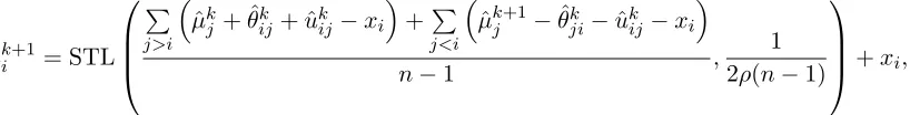
Using simple algebra and the soft thresholding operator for lasso (Tibshirani, 1996), we obtain an updating formula as:
ˆ
µk+1i = STL
P
j>i
ˆ
µkj + ˆθkij+ ˆukij−xi
+P
j<i
ˆ
µk+1j −θˆkji−uˆkij −xi
n−1 ,
1 2ρ(n−1)
+xi,
where STL(α, γ) = sign(α)(|α| −γ)+. In this case, the scalar operation on a vector is
element-wise.
In addition, we can also use other penalty functions. In an appendix, we provide details of the DC-ADMM algorithm for PRclust with lasso or TLP as grouping penalty.
2.4 Simulations
Consider two overlapped convex clusters with the same spherical shape in two dimensions. Specifically, a random sample of n = 100 observations was generated, with 50 from a bivariate Gaussian distribution N((0,0)0,0.33I), while the other 50 from N((1,1)
0
,0.33I), whereI is the identity matrix.
For PRclust, we searched τ ∈ {0.1,0.2, . . . ,1} and λ ∈ {0.01,0.05,0.1,0.2,0.3,0.5,0.7,
1,1.5,2}. To evaluate the performance of selecting the tuning parameters, we used the Rand index (Rand, 1971) and adjusted Rand index (Hubert and Arabie, 1985), measuring the agreement between estimated cluster and the truth with a higher value indicating a higher agreement. PRclust with the stability based criterion selecting its tuning parameters performed well: the average number of clusters was 2.63, slightly larger than the truth
K0 = 2; the correspond clustering results had high degrees of agreement with the truth,
as evidenced by the high indices. Table 1 shows the frequencies of the number of clusters selected by the stability criterion: for the overwhelming majority (93%), either the correct number of cluster K0 = 2 was selected, or a slightly larger K = 3 or 4 was selected.
As expected, applying the quadratic penalty based algorithm with the stability criterion yielded a similar result. GCV with GDF yielded the similar results for clustering accuracy. However, to use GCV with GDF, the user has to specify the perturbation size, a hyper-parameter. In contrast, the stability based criterion is insensitive to the repeat times T. For the simulation, the average numbers of clusters selected withT = 10,50 and 100 were 2.63, 2.68 and 2.76, respectively.
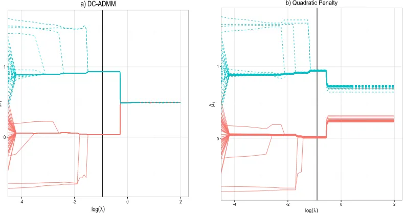
Now we illustrate differences between the two algorithms. First, we demonstrate how two algorithms operated differently with respect to various values of the tuning parameter
λ, whileτ was fixed at 0.7 (Figure 1). Note that, due to the soft constraint of the quadratic penalty based algorithm, we cannot obtain exactly ˆµi−µˆj−θˆij = 0. Even for a sufficiently
largeλ, there were still quite some unequal ˆµi,1’s, which were all remarkably close to their
true values 0 or 1. In contrast, due to using the hard constraint onθij =µi−µj, DC-ADMM
yielded some equal estimated centroids ˆµi,1. In this simulation, the stability based criterion
tended to select the most stable tuning parameters, confirming its selecting good tuning parameters and yielding good clustering results.
Stability Based Criterion GCV with GDF
Algorithm Freq Kˆ Rand aRand Freq Kˆ Rand aRand
DC-ADMM All 2.63 0.950 0.901 All 3.29 0.956 0.912
60 2.00 0.954 0.908 39 2.00 0.958 0.917
26 3.00 0.949 0.898 22 3.00 0.965 0.930
7 4.00 0.945 0.890 17 4.00 0.959 0.918
5 5.00 0.924 0.847 8 5.00 0.940 0.881
2 6.00 0.952 0.903 12 6.00 0.947 0.894
Quadratic All 2.70 0.951 0.902 All 2.41 0.962 9.925
Table 1: Comparison of the tuning parameter selection criteria based on 100 simulated data sets each with 2 clusters.
0
1
-4 -2 0 2
log(λ)
µ
^1
a) DC-ADMM
0 1
-4 -2 0 2
log(λ)
µ^1
b) Quadratic Penalty
Figure 1: Solution paths of the first coordinate ˆµi,1 for the first simulated data set. τ is
0 20000 40000
0 1000 2000 3000 4000 5000
Number of Observations
R un T ime (s) Methods DC-ADMM Quadtric Penalty
Log of Run Time
Log of Run Time O(pn2ε)
Run Time Run Time -5 0 5 10 Lo g of R un T ime (s) 0 100 200 300
0 25 50 75 100
Dimension R u n T ime (s) Methods DC-ADMM Quadtric Penalty
Log of Run time
Log of Run time
O(pn2ε) Run time
Run time -2 0 2 4 6 L o g o f R u n T ime (s)
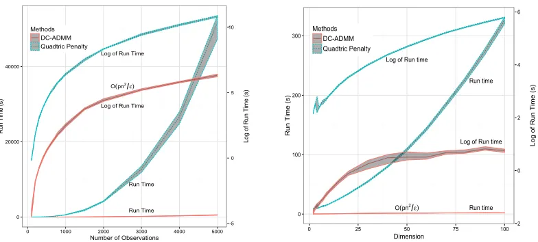
Figure 2: Comparison of run-times of DC-ADMM and quadratic penalty based algorithm based on the average of 100 simulations with different random seeds. Shaded regions represent the 25% and 75% quantiles of the run-times for corresponding algorithms. The complexity of DC-ADMM is O(pn2/), whereas the quadratic penalty based algorithm is much slower.
based algorithm, particularly when either n or p is large. For DC-ADMM, the number of iteration was insensitive to the sample size and was around 100. In contrast, for the quadratic penalty based algorithm, it increased dramatically as the sample size increased; when the sample size was 200, the number of iteration was around 1,000; however, the number of iteration increased to around 85,000 when the sample size increased to 6,000. The complexity of DC-ADMM is quadratic in the sample size n (the ratio of run-time to
n2 was around 10−5) and linear in the dimension p (the ratio of run-time top was around 0.05), confirming that the computational complexity isO(pn2/).
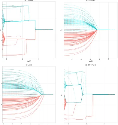
Figure 3 shows the solution paths for other methods. PRclust2 provided very similar results as DC-ADMM (Figure 3a). However, PRclust2 is extremely slow (around 10 to 30 times slower than the quadratic penalty based algorithm) and not feasible to large data sets. Convex penalties, such as the lasso and theL2-norm penalty, always shrink all the estimates
towards zero and thus lead to severely biased parameter estimates. For example, if we used the L2-norm (Figure 3b) or the lasso (Figure 3c) as the grouping penalty, the estimated
0 1
-4 -2 0 2
log(λ)
µ
^1
a) PRclust2
0 1
-7 -6 -5 -4 -3
log(λ)
µ
^1
b) L2 penalty
0 1
-9 -8 -7 -6 -5 -4
log(λ)
µ
^1
c) Lasso
0 1
-4 -2 0
log(λ)
µ
^1
d) TLP (τ=0.4)
Figure 3: Solution paths of ˆµi,1 for a) PRclust2, b) L2 penalty, c) Lasso penalty and d)
3. Theory
Though operating characteristics of PRclust have been intensively studied, its clustering consistency properties remain unknown. In this section, based on the maximum likelihood estimation framework, we develop some theoretical properties for penalized regression based clustering method, which incorporates original PRclust (Pan et al., 2013) as a special case. Recall that PRclust does not put any distribution assumptions on the data; however, it can be treated as assuming a Gaussian distribution for the data implicitly as to be shown later. To avoid unaddressable complexity of over-parameterizing the underlying distribu-tion, some mild technical assumptions are introduced. Then we develop a probability bound of clustering consistency which is slightly harder than clustering center consistency (Pollard, 1981).
3.1 PRclust in the Penalized Maximum Likelihood Framework
Assume xi ∈ Rp ∼ fµi(·), 1 ≤ i ≤ n are n independent random samples, where fµi is a probability density function of xi with its centroid µi ∈Rp. We obtain an estimate ˆµL0 of
µ= (µ01, . . . , µ0n)0 ∈Rpn via solving the following constrained L
0-problem:
minµ − L(µ) subject to J(µ)≤J, (7)
where J is a nonnegative tuning parameter controlling the trade-off between the model fit and the number of clusters,L(µ) =Pn
i=1log(fµi(xi)) is the log-likelihood that corresponds to the model fit, and J(µ) =P
i<jI{d(µi, µj) 6= 0} is the grouping penalty that controls
the number of clusters. I(·) is the indicator function andd(·,·) :Rp×Rp →Ris a distance, which can be defined d(µi, µj) =||µi−µj||q ={Ppm=1|µim−µjm|q}1/q, 0< q <∞. Then
J(µ) equals the number of distinct pairs of centroids µi6=µj.
The regularization problem (7) is a constrained counterpart of the following penalized unconstrained L0-problem:
minµ − L(µ) +λJ(µ), (8)
where λ≥0 is a tuning parameter corresponding to J in (8). Note that (7) and (8) may not be equivalent in their global minimizers, which is unlike a convex problem.
In a high-dimensional situation, it is not computationally feasible to minimize a discon-tinuous cost function in (8) and (7). As a surrogate, we consider an estimator ˆµtL1 that minimizes the following truncatedL1-problem:
minµ − L(µ) +λJτ(µ), (9)
whereJτ(µ) =Pi<jTLP(d(µi, µj);τ). Note that if assumingxi ∼M V N(µi, σ2I), 1≤i≤
nand usingL2-distance, we get−L(µ) =Pi=1n ||xi−µi||22after ignoring some constants and
Jτ(µ) =P
i<jTLP (||µi−µj||2;τ), which indicate that (9) reduces to the original PRclust
3.2 A Fundamental Assumption for Over-parameterization
To reduce the unaddressable complexity to an addressable level, we propose a fundamental assumption. Let Ck,1 ≤ k ≤ K be K clusters that satisfy ∪Kk=1Ck = {x1, . . . , xn} and Ci∩Cj =∅, for 1 ≤ i6= j ≤ K. The number of partitions of n samples into K clusters
is (1/K!)PK
k=1(−1)K−k Kk
kn, which in turn can be approximated by Kn/K! (Steinley,
2006). Since PRclust is based on over-parameterization and assumes one parameter (cen-troid) for one corresponding sample, the complexity of PRclust is the same as all possible ways of constructing clusters based on all samples. Unfortunately, to the best of our knowl-edge, there is no possible probability bound that can cover this complexity that requires tail probability decreasing faster than exp(−nlogK). However, many of the clustering for-mulation lead to the overlapped clusters and there is no way to reconstruct the true clusters exactly. To recover non-overlapped true clusters, we put a mild technical restriction on the clustering formulation to reduce the complexity.
Assumption (A0): Partition samples x1, x2, . . . , xn into K clusters. For any clusters C1, C2, . . . , CK, there exists m points y1(k), . . . , ym(k) ∈Ck such that d(y
(k)
m , xk) ≤d(y (k) m , xc)
for all xk ∈Ck andxc∈Ckc, where y(k)m =Pml=1yl/mand Ac denotes the complement of a
set A. We definem as theminimal disjoint centering number.
Note that all the clusters are separated under (A0). Violating (A0) implies that there exist xk ∈ Ck and xc ∈Ckc such that d(y(k)m , xk) > d(y
(k)
m , xc), indicating that there exists
another cluster that overlaps withCk. Interestingly, assumption of this kind seems necessary
because clustering consistency is impossible when some clusters overlap, although it appears strong. Worth of note is that other papers, for instance Zhu et al. (2014), explicitly assume that different clusters are reasonably separable from each other for clustering consistency. Furthermore, (A0) excludes any irregular cluster structures, which are not constructed. Most importantly, Lemma 1 in the Appendix gives an upper bound of the number of ways of reconstructable clusters under (A0), reducing the overparameterization complexity from the super-exponential level in the sample sizen, exp(−nlogK), to a polynomial level in n, exp(−mKlogn). Lastly, (A0) implies that all the clusters must include at least
m samples, and guarantees cluster-center consistency asymptotically: for each 1 ≤ k ≤
K,ky(k)m −µkk2 → 0 almost surely asm → ∞, where µk is the centroid of the cluster Ck.
Note that Pollard (1981) used a similar assumption for cluster-center consistency for the
k-means method.
3.3 Clustering Consistency for L0-constrained Problem
Define C = {C(µ) : µ ∈ Rpn}, where C(µ) = {C
1, . . . , CK} is a set of clusters based on µ
such that for any cluster Ck, d(µi, µj) = 0, ∀i, j ∈ Ck and d(µi, µj) 6= 0, ∀i∈ Ck, j ∈ Ckc.
Let µ∗ = (µ∗10, . . . , µn∗0)0 ∈ Rpn with µ∗
i = (µ∗i1, . . . , µ∗ip)
0
∈ Rp be the true centroid. We
study asymptotic properties of ˆµL0 in (7) by giving a bound of the incorrect clustering probability: P µˆL0 6= ˆµo
, where ˆµo = (ˆµo10, . . . ,µˆno0)0 = argminC(µ)=C(µ∗)L(µ) is the oracle
estimator that is usually unavailable unless the true clusters are known beforehand. Note that ˆµL0 is defined as a global minimizer of (7) and assume to be any global minimizer.
smallest size. To be specific, let S(,F, r) ={f1l, f1u, . . . , frl, fru}be the bracket covering of F that satisfies max1≤j≤r||fju−fjl||2 ≤ , where ||f||2 = (
R
f2dv)1/2 and there exists a j
such that fjl ≤f ≤fju for any f ∈ F, then H(,F) = log(min{r :S(,F, r)}). For more discussions about metric entropy of this type, see Kolmogorov and Tikhomirov (1959). To construct the clustering consistency properties, we need the following two assumptions.
Assumption (A1): There exists some constant d0 >0 such that, for any >0,
supC∈C:|C|≤|C(µ∗)|H(t,FC)≤d0mlog(n) log(2/28t), 2/28 < t <21/2≤1,
where FC = {fµ : h2a(fµ, fµ∗) ≤ 2, µ ∈ BC}, fµ is the density of x = (x 0
1, . . . , x
0
n)
0
, BC = {µ : C(µ) = C}, |A| is the cardinality of a set A and m is the minimal disjoint
centering number defined in (A0).
Note that (A1) puts some constraints on the size of parameter space, which is similar as Assumption A in Shen et al. (2012) and is a direct modification of the assumption in Wong and Shen (1995).
Define
Cmin(µ∗)≡ inf µ∈B
h2
a(fµ, fµ∗)
|C(µ)|
to be the degree-of-separation or the level of difficulty of clustering, whereB={µ:C(µ)6= C(µ∗),J(µ)≤ J(µ∗)} is a parameter space of interest,ha(fµ, fµ∗) =Pn
i=1h(fµi, fµ∗i)/n
1/2
is the averaged Hellinger metric withh(fµi, fµ∗i) =
n
1 2
R
(fµ1/2i −f
1/2 µ∗i )2dv
o1/2
.
Assumption (A2): There exists some constant d1 >0 such that
Cmin(µ∗)> d1mlog(n)/n,
wherem is the minimal disjoint centering number defined in (A0).
Assumption (A2) describes the least favorable situation through Cmin(µ∗) under which
we can identify the true cluster partition. In fact,Cmin(µ∗) depends on the number of true clusters and the minimum distance among true cluster centers induced by the Hellinger loss. Since (A2) puts some regularity conditions on log-likelihood function via Hellinger loss, we do not make any regularity conditions for the log-likelihood function explicitly. Similar assumptions as (A2) can be found in the literature of feature selection. For example, Shen et al. (2012) assumed
Cmin(β∗)≥d0log(p)/n, (10)
whereβ∗ is a true parameter vector of interest,d0 is a positive constant,pis the dimension
of β and n is the sample size. By assuming a probabilistic model such as the Gaussian distribution, (10) can be further specified as
γ2min= min
j:β∗
j6=0
|β∗j| ≥d0log(p)/n,
which implies the feature selection consistency can be constructed even when the minimal signal size is vanishing γmin → 0 and the dimension of features is diverging p → ∞. This
assumption is much weaker than classical assumptions where γmin and p are usually fixed
(A2) serves similar roles for clustering consistency as (10) for feature selection consis-tency. As to be shown later in Proposition 1, by assuming the Gaussian distribution, (A2) can be explicitly specified. More importantly, it allows the minimum distance among dif-ferent cluster centroids decreases toward zero, αmin = minµ∗
i6=µ∗jkµ
∗
i −µ∗jk2 → 0, and the
number of cluster diverge to infinity, K → ∞, indicating that the assumption used here is weaker than many other studies where αmin and K are usually fixed constants (Pollard,
1981; Pelckmans et al., 2005; Radchenko and Mukherjee, 2014; Zhu et al., 2014). Then we establish the main theory for clustering consistency as follows.
Theorem 2 Under Assumptions (A0) to (A2), if J = J(µ∗), then, there exists some
constant c2 >0, such that
P µˆL0 6= ˆµo
≤exp (−c2nCmin(µ∗) + (m+ 1) log(n) + 2),
provided thatd1 >max{1/c2,2d0(logc3)/c24}. For example, we may usec2= 4/(27×1926),
c3 = 10 and c4 = (2/3)5/2/512. Further, µˆL0 reconstructs the oracle estimator µˆo with
probability tending to one as n→ ∞. The following two asymptotic results hold asn→ ∞:
(A) (Clustering consistency) P(ˆµL0 6= ˆµo)→0 and hence P C(ˆµL0)6=C(ˆµ∗)→0.
(B) (Optimal parameter estimation)E
h2a(fµˆL0, fµ∗)= (1+o(1))Eh2a(fµˆo, fµ∗), provided
thatc2nCmin(µ∗) + log E
h2a(fµˆo, fµ∗)→ ∞.
Theorem 2 says that, under Assumptions (A0) to (A2), ˆµL0 consistently reconstructs the oracle estimator ˆµo, and both an oracle clustering and an optimal parameter estimation with respect to expected Hellinger risk are asymptotically available by solving a constrained
L0-problem. As pointed out by a reviewer, the number of clusters K is an important but
unknown tuning parameter. Theorem 2 shows that if the tuning parameter J is chosen to beJ =|J(µ∗)|then optimal clustering can be constructed asymptotically. We believe that theory established here can be a starting point in developing some new tuning parameter selection criteria, though we have not fully explored in this aspect here. Theorem 2 provides an insight into or gives theoretical justification on when or under which condition the proposed method is expected to give correct clustering. For instance, the theory suggests that the optimal tuning parameters may depend on the underlying true parameters, which needs to be estimated for real data. This, together with the tuning parameter selection criterion lead to the estimated data-dependent tuning parameter for this real data set.
Although theoretical properties of penalized clustering have been intensively studied (Radchenko and Mukherjee, 2014; Zhu et al., 2014), our result is new and different from the proceeding ones. For example, Radchenko and Mukherjee (2014) proved clustering consistency with univariate samples, which are not practical and, in fact, relatively easy to prove in our context without assumption (A0) since the complexity of over-parametrization falls down to an addressable level. Zhu et al. (2014) extended the clustering consistency to multivariate samples by assuming there are only two clusters, sayC1 and C2 with centroids µ1 and µ2, respectively. To avoid some technical difficulties, Zhu et al. (2014) imposed an
assumption that is not required in Theorem 2: two clustersC1 andC2 consist proportional
number of samples in the sense that|C1|/|C2| →c, wherecis a positive constant. Theorem
3.4 Example: Truncated Multivariate Gaussian Distributions
In this example, we give a sufficient condition for (A2) to hold asymptotically, by con-structing a lower bound of Cmin(µ∗) in terms of the minimum center distance αmin =
minµ∗i6=µ∗jkµ∗i−µ∗jk2. Letφµi,1≤i≤nbe the multivariate Gaussian density function with mean µi ∈ Rp and identity covariance matrix Ip×p, that is, φµi(z) = (2π)
−p/2exp(−kz− µik22/2), z ∈ Rp,1 ≤ i ≤ n. For notation simplicity, we denote φµi = φ when µi = 0. Note that it is not generally anticipated for clustering consistency under the usual Gaussian distribution assumption since the Gaussian distribution leads to overlapped clusters and violates the assumption (A0). Hence we modify the underlying distributions for the results in Theorem 2 by considering non-overlapping situations.
Consider a class of the truncated densitiesφµi,α,1≤i≤nwith a truncation levelα >0:
φµi,α(z) = (1/cα)φµi(z)I kz−µik
2 2 ≤α/4
, (11)
wherecα is a normalizing constant. Note thatcα=
R
Aµi,αφµi(z)dz =
R
Aαφ(z)dz =χp(α/4), where Aµi,α = {z : kz−µik
2
2 ≤ α/4}, Aα = {z : kzk22 ≤ α/4} and χp is the chi-square
distribution function withpdegrees of freedom. Given two mean vectorsµi 6=µj,φµi,αdoes not overlap with φµj,α ifkµi−µjk
2
2 > α. Since the truncated densitiesφµi,α for 1≤i≤n in (11) are not overlapped to each other if we take α = αmin = minµi=µ6 jkµi −µjk
2 2,
we assume that the samples are independently distributed with true truncated densities
φµ∗i,αmin; 1≤i≤nwith a truncation levelαmin.
Now, ignoring constants, consider the problem in (7) for minimizing the minus log-likelihood −L(µ) = Pn
i=1kxi −µik22/2 under the constraint J(µ) ≤ J. To derive a
suf-ficient condition for (A2), we construct a lower bound of Cmin(µ∗), the level of difficulty
in recovering C(µ∗). Asymptotic properties cannot be established when cluster Cj ∈ C(µ)
only shares a finite number of samples with true clusters, and thus we make the following assumption.
Assumption (A3): For any µ∈Rnp, there existsm
1 such that infC∈C(µ),C∗∈C(µ∗),C∩C∗6=∅
|C∩C∗| ≥m1.
Proposition 1 Letrαmin ={infµ∈Binfαmin−kµi−µ∗ik22≤t≤αminχp(t/4)}/{4χp(αmin/4)}, where
χp and χp are the chi-square density and distribution functions with p degrees of freedom,
respectively. Under assumptions (A0), (A1) and (A3), if J = J(µ∗) then the consistency
results (A) and (B) in Theorem 2 hold, provided that
rαminαmin≥d1mK∗log(n)/m1, (12)
for some constants d1 >max{1/c2,2d0log(c3)/c24}, where K∗ =|C(µ∗)|.
Proposition 1 implies that (12) is a sufficient condition for (A2) for the truncated multivariate Gaussian distributions. In low dimensional situation, αmin, p and K∗ may
be fixed. rαmin is bounded below, which implies the clustering consistency follows when
mlog(n)/m1 → ∞ asn→ ∞. Moreover, clustering consistency holds when αmin → 0 and
p → ∞. From L’Hpital’s rule, limαmin→0rαmin ≤ limαmin→0χp(αmin/4)/4χp(αmin/4) = ∞
for any p ≥3, which implies (12) is satisfied when m1αmin/mK∗log(n) → ∞as n → ∞.
For example, let K∗log(n) = nk, m = nh and m1 = nh1 for some positive constants k, h
implying that we can recover the true clusters even whenαmin →0 andK∗→ ∞asn→ ∞
for any p≥3.
At first sight, a truncated multivariate Gaussian distribution is an extreme example; however, after ignoring some constants the corresponding minus log-likelihood function −L(µ) = Pn
i=1||xi −µi||22, is used in the original PRclust. Moreover, truncated
multi-variate Gaussian distributions guarantee that different clusters are separated from each other; non-truncated Gaussian distributions lead to overlapping clusters, and consistency of distance-based clustering methods, including ours, is not expected as a result. For exam-ple, suppose we have n observations, n/2 form a Gaussian distribution N(−0.5,1), while the othern/2 from N(0.5,1). According to the K-means cluster center consistency theory (Pollard, 1981), the cluster centers determined by the K-means with K = 2 converge to
a1 = −0.9 and a2 = 0.9, not the original clusters centers at µ1 = −0.5 and µ2 = 0.5.
The reason is that all the negative observations from the second distribution/cluster are mis-clustered into the first cluster, while all positive observations from the first clusters are incorrectly assigned to the second cluster by the K-means, leading to an under-estimated center for the first cluster; similarly the over-estimation of the second cluster center can be explained. This simple example suggests that clustering consistency cannot be established when non-truncated Gaussian distributions are used in K-means. Furthermore, previous works focused on establishing clustering consistency with the distance between clusters growing at a sufficiently fast rate. For example, Zhu et al. (2014) showed that if the dis-tance between two clusters and sample size n grow at the same rate asn → ∞, then the corresponding method can separate the two clusters perfectly. In contrast, clustering con-sistency established here still holds when minimum distance between the cluster centroids
αmin →0 , implying that the assumptions used here are weaker than the previous ones.
4. Discussion
The proposed new algorithm DC-ADMM bears some similarity to the quadratic penalty based algorithm in terms of the cost function and using difference convex programming. However, they differ significantly in their specific formulations. Instead of using the quad-ratic penalty technique, we use a hard constraint and an augmented Lagrangian in DC-ADMM. Consequently, the DC-ADMM is much faster than the quadratic penalty based algorithm and can be relatively easy to be extended to other cost functions that may have some advantages for certain problems.
The theory that states some sufficient conditions for clustering consistency and optimal parameter estimation in the PRclust framework covers a much wide range of loss functions and grouping penalties, which helps us study theoretical results uniformly for some specific PRclust implementations in the future. For example, when graph information is available, by adding a constraint on the two connected nodes in the graph, we can estimate a clus-ter partition and grouping structure of variables simultaneously. The mis-clusclus-tering error bound and asymptotic properties of this graph-based PRclust can be obtained via a slight modification to the theory established here.
over-relaxed ADMM algorithm to speed up. Other options exist; for example, we may use different values of ρ in each iteration (Wang and Liao, 2001). Second, since the algorithm is relatively fast, it is now feasible to deal with high dimensional data, for which variable selection is necessary. In principle, we may add a new penalty into the cost function for variable selection (Pan and Shen, 2007). Third, we may modify PRclust for noisy big data. Others have developed an iterative sub-sampling approach to improve the computational efficiency of a solution path clustering and to handle noisy big data (Marchetti and Zhou, 2014). A modification of PRclust along this direction may be useful.
An R packageprclustimplementing the DC-ADMM algorithm and the quadratic penalty algorithm with various loss and penalty functions is available at GitHub (https://github.
com/ChongWu-Biostat/prclust) and CRAN (http://cran.r-project.org).
Acknowledgments
Appendix A.
Proof of Theorem 1. The finite termination property of DC-ADMM follows from the following three facts. First, since (2) is closed, proper and convex and the augmented Lagrangian (4) has a saddle point, the standard ADMM converges (Boyd et al., 2011). Second, by construction ofS(m)(µ, θ), for eachm∈N,
0≤S(ˆµ(m),θˆ(m)) =S(m+1)(ˆµ(m),θˆ(m))≤S(m)(ˆµ(m),θˆ(m)) ≤S(m)(ˆµ(m−1),θˆ(m−1)) =S(ˆµ(m−1),θˆ(m−1)),
implying that S(ˆµ(m),θˆ(m)) decreases in m; otherwise the algorithm stops. Note that (ˆµ(m),θˆ(m)) is the limiting point of the ADMM iterations in (5). Third, since S(m+1)(µ, θ) depends on m only through that on the indicator functions I(||θˆ(m)ij ||2 < τ), which can be either 1 or 0, S(m+1)(µ, θ) has only a finite set of possible functional forms across all m, leading to a finite number of its possible and distinct minimal values. These facts imply that DC-ADMM terminates in a finite number of iterations.
To show that (ˆµ(m∗),θˆ(m∗)) is a KKT point ofS(µ, θ), we check if the solution satisfies a local optimality ofS(µ, θ). Since the subgradient ofS(µ, θ) andSm(µ, θ) are the same at the minimizer (Rockafellar, 2015), we verify the following requirement:
xi+ρ
X
j>i
(µj+θij+uij) +ρ
X
j<i
(µj−θji−uij)−(1 +ρ(n−1))µi = 0; (13)
λbijθij/||θij||2+ρ(θij −(µi−µj) +uij) = 0; (14)
θij −µi−µj = 0, (15)
where bij is the regular subdifferential of min(||θij||2, τ) at||θij||2. Easily, (15) is the hard
constraint in the DC-ADMM and is met at convergence. Note that (ˆµ(m∗),θˆ(m∗),uˆ(m∗)) = (ˆµ(m∗−1),θˆ(m∗−1),uˆ(m∗−1)) at termination. Then (13) is satisfied with (µ, θ, u) = (ˆµ(m∗−1),
ˆ
θ(m∗−1),uˆ(m∗−1)). For (14), consider three cases.
• If ||θˆ(m
∗−1)
ij ||2 > τ, the ˆθ (m∗−1) ij = ˆµ
(m∗) i −µˆ
(m∗) j −u
(m∗)
ij , implying θij = ˆθ (m∗) ij since bij = 0.
• If 0<||θˆij(m∗)||2 < τ and ||µˆ(m
∗)
i −µˆ (m∗)
j −uˆ (m∗)
ij ||2 > λ/ρ, then
ˆ
θ(m
∗)
ij =
||µˆ(m
∗)
i −µˆ (m∗) j −uˆ
(m∗) ij ||2−
λ ρ
µˆ(m
∗)
i −µˆ (m∗)
j −uˆ (m∗)
ij
||µˆ(mi ∗)−µˆj(m∗)−uˆ(mij ∗)||2, hence that||θˆ(mij ∗)||2=||ˆµ(m
∗)
i −µˆ (m∗) j −uˆ
(m∗)
ij ||2−λρ. Then (14) is met whenθij = ˆθ(m
∗)
ij
sincebij = 1.
• If 0 <||θˆ(m
∗)
ij ||2 < τ and ||ˆµ (m∗) i −µˆ
(m∗) j −uˆ
(m∗)
ij ||2 < λ/ρ, then||θˆ (m∗)
ij ||2 = 0, which
This completes the proof.
Lemma 1. Given n observations xi ∈ Rp, 1 ≤ i ≤ n, let the number of ways of
constructing K clusters that satisfies disjoint condition (assumption A0) with the minimal
disjoint centering number m be cn,K,m. Then
cn,K,m≤(n−Km)K K
Y
k=1
n−(k−1)m m
.
Proof of Lemma 1. Without loss of generality, we fix the first km points and form K
disjoint subsets Sk ={x(k−1)m+1, . . . , xkm} ⊂ {x1, . . . , xn}, k ≤K. Let r (k) i = d(x
(k) m , xi), km+ 1 ≤ i ≤ n with x(k)m = Pkmj=(k−1)m+1xj/m and ˜ri(k) be an ordered sequence of r
(k) i
that satisfies ˜r(k)km+1 ≤ · · · ≤ r˜(k)n . Then a possible way of constructing a subset Ck based
on Sk is including Sk and all the points within distance ˜r (k)
i . For a subset Ck, the number
of constructing ways is n−Km at most. Hence, the number of ways of constructing K
subsets Ck,k≤K based on Sk is (n−Km)K at most.
Note that the number of ways of fixing possible K disjoint subsets Sk, k ≤ K is
QK
k=1
n−(k−1)m m
. Hence the total number of ways of constructing K subsets along to the way described above is (n−Km)KQK
k=1
n−(k−1)m m
at most. Note that any clus-ter partition with K clusters that satisfies disjoint structure condition with the minimal
disjoint centering number m can be constructed via the ways described above. Hence
cn,K,m≤(n−Km)KQKk=1 n−(km−1)m
. This completes the proof.
Proof of Theorem 2. On the set ˜B = {µ : C(µ) = C(µ∗)} ⊂ {µ : J(µ) ≤ J(µ∗)}, we have ˆµL0 = supµ∈B˜L(µ) = ˆµo = supC(µ)=C(µ∗)L(µ). Let the parameter space of interest be
B={µ:C(µ)6=C(µ∗),J(µ)≤ J(µ∗)}. Since J(µ)≤ J(µ∗) implies |C(µ)| ≤K∗, we have B ⊂ {µ:C(µ) 6= C(µ∗),|C(µ)| ≤K∗} ⊂ ∪K∗
k=1∪C∈CkBC, where BC ={µ :C(µ) =C} and Ck={C ∈ C:C 6=C(µ∗),|C|=k}. Hence, usingL(ˆµo)≥ L(µ∗), we have
P µˆL0 6= ˆµo≤P∗ sup
µ∈B
{L(µ)− L(ˆµo)}>0
!
≤P∗ sup
µ∈B
{L(µ)− L(µ∗)}>0
!
≤
K∗
X
k=1
X
C∈Ck
P∗ sup
µ∈BC
{L(µ)− L(µ∗)}>0
!
,
where P∗ is the outer probability. Now we apply Theorem 1 of Wong and Shen (1995) to bound each term. For any µ ∈ BC and C ∈ Ck, h2a(fµ, fµ∗) ≥ kCmin(µ∗), there exists a
constantc2 >0 such that P∗ sup
µ∈BC
{L(µ)− L(µ∗)}>0
!
provided that the local entropy conditions are satisfied as follows: there exist constants
c3 >0 andc4>0 such that
Z 21/2
2/28
H1/2(t/c3,FC)dt≤c4n1/22 (16)
for any 2 ≥ kCmin(µ∗). Let 2n = 2d0log(c3)mlog(n)/c24n. Under (A1), n solves the
inequality
max
k≤K∗ sup
C∈Ck
Z 21/2 2/28
H1/2(t/c3,FC)dt≤(d0mlog(n))1/2(21/2)(log(c3))1/2 ≤c4n1/22
with respect toprovided thatn< . Hence, (16) follows ifCmin(µ∗)≥2n, and from (A2),
this holds whend1≥2d0log(c3)m/c24. From Lemma 1,|Ck| ≤(n−km)k
Qk
j=1
n−(j−1)m m
≤
nk+mk. Hence,
P µˆL0 6= ˆµo
≤
K∗
X
k=1
4 exp (−c2nkCmin(µ∗) +k(m+ 1) log(n))
≤4R(exp(−c2nCmin(µ∗) + (m+ 1) log(n))
≤5 exp (−c2nCmin(µ∗) + (m+ 1) log(n))
≤exp (−c2nCmin(µ∗) + (m+ 1) log(n) + 2),
whereR(x) =x/(1−x) is exponentiated logistic function. Now (A) follows from P C(ˆµL0 6=C(µ∗)
≤P µˆL0 6=µ∗
and d1 > 1/c2. For the risk
property, using h2a(ˆµL0, µ∗)≤1,
E
h2a(ˆµL0, µ∗)
≤E
h2a(ˆµo, µ∗)
+E
h2a(ˆµL0, µ∗)I(ˆµL0 6= ˆµo)
≤E
h2a(ˆµo, µ∗)
+P(ˆµL0 6= ˆµo) ≤(1 +o(1))Eh2a(ˆµo, µ∗)
provided that exp (−c2nCmin(µ∗))/Eh2a(ˆµo, µ∗) =o(1), and then (B) established. This
com-pletes the proof.
Proof of Proposition 1. It suffices to show that (12) is a sufficient condition for As-sumption (A2). First, we give a lower bound of the Hellinger metric between φµi,αmin and
φµ∗
i,αmin for a givenµ∈ B ={µ:C(µ)6=C(µ
∗),J(µ)≤ J(µ∗)}. Let
Aαmin ={z:kzk22≤αmin/4} and Aµi,αmin ={z:kz−µik
2
Givenµi 6=µ∗i withkµi−µ∗ik22 ≤αmin, let ∆∗i =µi−µ∗i then we have h2(φµi,αmin, φµ∗i,αmin)
2
=h2(φαmin, φ∆∗,αmin)2
=1 2
Z
φ1/2αmin(z)−φ1/2∆∗
i,αmin(z)
2
dz
= 1
2χ2
p(αmin/4)
Z
Aαmin
φ(z)dz+
Z
A∆∗
i,αmin
φ∆∗i(z)dz−2
Z
Aαmin∩A∆∗
i,αmin
φ(z)1/2φ∆∗(z)1/2dz
!
= 1
χ2
p(αmin/4)
Z
Aαmin
φ(z)dz−
Z
Aαmin∩A∆∗
i,αmin
φ(z)1/2φ∆∗(z)1/2dz
!
.
LetB∆∗i,αmin ={z:kz−∆i∗k22≤α/4− k∆∗ik22/4} then it is easy to see that Aαmin ∩A∆∗i,αmin ⊂B∆∗i,αmin.
By using the equality,
φ(z)1/2φ∆∗i(z)1/2 = (2π)−p/2exp(−kz−∆i∗/2k22/2− k∆∗k22/8) = exp(−k∆∗ik22/8)φ∆∗
i/2(z),
we have
Z
Aαmin∩A∆∗
i,αmin
φ(z)1/2φ∆∗(z)1/2dz ≤exp(−k∆∗
ik22/8)
R
B∆∗
i,αmin
φ∆∗
i/2(z)dz
= exp(−k∆∗ik22/8)χp(αmin/4− k∆∗ik22/4)
≤χp(αmin/4− k∆∗ik22/4).
According to the mean value theorem,
h2(φµi,αmin, φµ∗i,αmin)
2≥ χp(αmin/4)−χp(αmin/4− k∆∗ik22/4)
χ2
p(αmin/4)
≥rαminkµi−µ∗ik22, (17)
where rαmin = {infµ∈Binfαmin−k∆∗ik2
2≤t≤αminχp(t/4)}/4χp(αmin/4). Next, we find a lower
bound ofCmin(µ∗). From (17), the inequalityh2a(fµ, fµ∗)≥Pn
i=1h2(fµi, fµ∗i)/n implies
nCmin(µ∗) =ninf µ∈Bh
2
a(fµ, fµ∗)/|C(µ)| ≥nrα∗ inf
µ∈Bkµ−µ ∗k2
2/|C(µ)|. (18)
It is easy to see that infµ∈{µ:|C(µ)|<K∗}kµ−µ∗k22/|C(µ)| ≥infµ∈{µ:|C(µ)|=K∗}kµ−µ∗k22/K∗,
since the sum of within cluster variances,kµ−µ∗k2 2 =
Pn
i=1kµi−µ
∗
ik22, is minimized when
|C(µ)|=K∗. Hence, we have
inf
µ∈Bkµ−µ ∗k2
2/|C(µ)|= infµ∈{µ:|C(µ)|=K∗,C(µ)6=C(µ∗)}kµ−µ∗k22/K∗. (19)
Let C(µ) ={C1, . . . , CK} and C(µ∗) ={C1∗, . . . , CK∗∗}. SinceC(µ)6=C(µ∗), without loss of
generality, we may assume thatCs∩Ct∗6=∅fors, t= 1,2. Then the right-hand side of (19)
∪3≤k≤K∗Ck}. Let µi =νs, i∈Cs fors= 1,2 and similarly let µ∗
i =νt∗, i∈Ct∗ fort= 1,2.
Then it follows that
inf
µ∈Bkµ−µ ∗k2
2 = inf µ∈B12
X
t=1,2
n1tkν1−νt∗k22+n2tkν2−νt∗k22
= inf
nst,s,t=1,2
X
t=1,2
n1tk¯ν1∗−νt∗k22+n2tk¯ν2∗−νt∗k22
= inf
nst,s,t=1,2
n11n12 n11+n12
+ n21n22
n21+n22
kν1∗−ν2∗k2 2,
wherenst =|Cs∩Ct∗|fors, t= 1,2, and ¯ν1∗= (n11ν1∗+n12ν2∗)/(n11+n12) and ¯ν2∗ = (n21ν1∗+ n22ν2∗)/(n21+n22) are the weighted means ofν1∗s andν2∗s in C1 and C2, respectively. From
(A3),nst ≥m1fors, t= 1,2, which impliesn11n12/(n11+n12) = 1/(1/n11+ 1/n12)≥m1/2
and similarly,n21n22/(n21+n22)≥m1/2. Hence the lower bound becomes
inf
µ∈Bkµ−µ ∗k2
2≥m1αmin. (20)
From (18), (19), (20) and definition of Cmin(µ∗), it is easy to see that (A2) is met if Cmin(µ∗)≥rαminm1αmin/nK∗ ≥d1mlog(n)/nwhich is equivalent to
rαminαmin≥d1mK∗log(n)/m1.
This completes the proof.
Appendix B.
The cost function of PRclust with lasso grouping penalty will be convex, and thus DC-ADMM is exactly same as DC-ADMM and a global solution will be reached. Note thatθij =
(θij1, . . . , θijp)
0
, then the updating formulas can be summarized as follows:
ˆ
µ(m+1)i =
xi+ρP j>i
ˆ
µ(m)j + ˆθ(m)ij + ˆu(m)ij +ρP
j<i
ˆ
µ(m+1)j −θˆ(m)ji −uˆ(m)ij
1 +ρ(n−1) ;
ˆ
θijl(m+1)= STµˆ(m+1)il −µˆ(m+1)jl −uˆ(m)ijl ;λ/ρ
ˆ
u(m+1)ij = ˆu(m)ij + ˆθij(m+1)−(ˆµ(m+1)i −µˆ(m+1)j ), 1≤i < j ≤n;i, l= 1,2, . . . , p.
The main difference between TLP and gTLP is that TLP is an element-wise penalty and the updating formulas (5) for PRclust with TLP can be summarized as follows, while the other part of DC-ADMM remains unchanged:
ˆ
µk+1i =
xi+ρP j>i
ˆ
µkj + ˆθijk + ˆukij+ρP
j<i
ˆ
µk+1j −θˆkji−uˆmij
1 +ρ(n−1) ;
ˆ
θijkk+1=
ˆ
µk+1il −µˆk+1jl −uˆk
ijl if |θˆ (m) ijl | ≥τ;
STL
ˆ
µk+1il −µˆk+1jl −uˆkijl;λ/ρ
if |θˆijl(m)|< τ; ˆ
References
Stephen Boyd, Neal Parikh, Eric Chu, Borja Peleato, and Jonathan Eckstein. Distributed optimization and statistical learning via the alternating direction method of multipliers.
Foundations and Trends in Machine Learning, 3(1):1–122, 2011.
Leo Breiman and Adele Cutler. A deterministic algorithm for global optimization.
Mathe-matical Programming, 58(1-3):179–199, 1993.
Eric C Chi and Kenneth Lange. Splitting methods for convex clustering. Journal of
Com-putational and Graphical Statistics, 24(4):994–1013, 2015.
Euhanna Ghadimi, Andr´e Teixeira, Iman Shames, and Mikael Johansson. Optimal pa-rameter selection for the alternating direction method of multipliers (admm): quadratic problems. IEEE Transactions on Automatic Control, 60(3):644–658, 2015.
Bingsheng He and Xiaoming Yuan. On non-ergodic convergence rate of douglas–rachford alternating direction method of multipliers. Numerische Mathematik, 130(3):567–577, 2015.
Toby Dylan Hocking, Armand Joulin, Francis Bach, and Jean-Philippe Vert. Clusterpath an algorithm for clustering using convex fusion penalties. In 28th International Conference
on Machine Learning (ICML), 2011.
Lawrence Hubert and Phipps Arabie. Comparing partitions. Journal of Classification, 2 (1):193–218, 1985.
Anil K Jain. Data clustering: 50 years beyond k-means. Pattern Recognition Letters, 31 (8):651–666, 2010.
Andrei Nikolaevich Kolmogorov and Vladimir Mikhailovich Tikhomirov. ε-entropy and
ε-capacity of sets in function spaces. Uspekhi Matematicheskikh Nauk, 14(2):3–86, 1959.
An Le Thi Hoai and Pham Dinh Tao. Solving a class of linearly constrained indefinite quadratic problems by dc algorithms. Journal of Global Optimization, 11(3):253–285, 1997.
Fredrik Lindsten, Henrik Ohlsson, and Lennart Ljung. Clustering using sum-of-norms reg-ularization: With application to particle filter output computation. In Statistical Signal
Processing Workshop, 2011.
Binghui Liu, Xiaotong Shen, and Wei Pan. Integrative and regularized principal component analysis of multiple sources of data. Statistics in Medicine, 35(13):2235–50, 2016.
Yuliya Marchetti and Qing Zhou. Iterative subsampling in solution path clustering of noisy big data. arXiv preprint arXiv:1412.1559, 2014.
Wei Pan, Xiaotong Shen, and Binghui Liu. Cluster analysis: unsupervised learning via su-pervised learning with a non-convex penalty. The Journal of Machine Learning Research, 14(1):1865–1889, 2013.
Kristiaan Pelckmans, Joseph De Brabanter, JAK Suykens, and B De Moor. Convex clus-tering shrinkage. In PASCAL Workshop on Statistics and Optimization of Clustering
Workshop, 2005.
David Pollard. Strong consistency of k-means clustering. The Annals of Statistics, 9(1): 135–140, 1981.
Peter Radchenko and Gourab Mukherjee. Consistent clustering using anl1 fusion penalty.
arXiv preprint arXiv:1412.0753, 2014.
William M Rand. Objective criteria for the evaluation of clustering methods. Journal of
the American Statistical Association, 66(336):846–850, 1971.
Ralph Tyrell Rockafellar. Convex Analysis. Princeton university press, 2015.
Xiaotong Shen, Wei Pan, and Yunzhang Zhu. Likelihood-based selection and sharp pa-rameter estimation. Journal of the American Statistical Association, 107(497):223–232, 2012.
Douglas Steinley. K-means clustering: a half-century synthesis. British Journal of
Mathe-matical and Statistical Psychology, 59(1):1–34, 2006.
Robert Tibshirani. Regression shrinkage and selection via the lasso. Journal of the Royal
Statistical Society: Series B, 58(1):267–288, 1996.
Robert Tibshirani and Guenther Walther. Cluster validation by prediction strength.Journal
of Computational and Graphical Statistics, 14(3):511–528, 2005.
S.L. Wang and L.Z. Liao. Decomposition method with a variable parameter for a class of monotone variational inequality problems. Journal of Optimization Theory and
Applica-tions, 109(2):415–429, 2001.
Wing Hung Wong and Xiaotong Shen. Probability inequalities for likelihood ratios and convergence rates of sieve mles. The Annals of Statistics, 23(2):339–362, 1995.
Rui Xu, Donald Wunsch, et al. Survey of clustering algorithms. Neural Networks, IEEE
Transactions on, 16(3):645–678, 2005.
Ming Yuan and Yi Lin. Model selection and estimation in regression with grouped variables.
Journal of the Royal Statistical Society: Series B, 68(1):49–67, 2006.